Adaptive large neighborhood search for multi-trip vehicle routing with time windows

Adaptive large neighborhood search for multi-trip vehicle routing

with time windows

V´

eronique Fran¸cois

_{, Yasemin Arda}

_{, and Yves Crama}

_{HEC Li`}

_{ege - Management School of the University of Li`}

_ege

Abstract

We consider a multi-trip vehicle routing problem with time windows (MTVRPTW), in which each vehicle can perform several trips during its working shift. This problem is especially relevant in the context of city logistics. Heuristic solution methods for multi-trip vehicle routing problems often separate routing and assignment phases in order to create trips and then assign them to the available vehicles. We show that this approach is outperformed by an integrated solution method in the presence of time windows. We use an automatic configuration tool to obtain efficient and contextualized implementations of our solution methods. We provide suitable instances for the MTVRPTW as well as an instance generator. Also, we discuss the relevance of two objective functions: the total duration and the total travel time. When minimizing the travel time, large increases of waiting time are incurred, which is not realistic in practice.

1

Introduction

In a multi-trip vehicle routing problem (MTVRP), each vehicle performs a set of trips, whose total du-ration, corresponding to the vehicle travel time, is limited by the length of the planning horizon. In a multi-trip vehicle routing problem with time windows (MTVRPTW), customers must be served within a specified time window and the duration of a set of trips assigned to a vehicle is usually bounded by the length of the depot’s time window which corresponds to the planning horizon. These two problems are common in city distribution systems (Cattaruzza et al., 2017). In urban areas, small vehicles are encour-aged for environmental reasons and, in most cases, required due to accessibility restrictions, limiting the loading capacity of the vehicles. Moreover, travel times between delivery points are short compared to the planning horizon, allowing vehicles to return to the depot several times for reloading. In this context, multiple trips arise naturally. They are also common when products are ready for delivery at different

points in time to be distributed on the same day. This is for example the case in nuclear medicine delivery (Lee et al., 2014) and home chemotherapy systems (Kergosien et al., 2017), since products are highly perishable and have to be delivered as early as possible after their production.

In this article, we study an MTVRPTW with a given fleet size and driver shifts shorter than the planning horizon. This operational problem is common in many distribution systems with a one-day planning period. Indeed, to increase the satisfaction of customers, or to avoid traffic jams, some deliveries have to be performed in the early morning, and some others in the late evening, implying that each driver can only cover a portion of the planning period. The driver shifts we consider have a limited duration and are not fixed in time, i.e., the start time of each shift is a decision variable.

Additionally, we minimize the total working duration, which includes the travel time, the waiting time as well as loading and service times, instead of the most employed objective function, i.e., the total travel time. Indeed, waiting times may induce direct or indirect costs linked to specialized equipment. In the particular case of refrigerated urban distribution, the negative impact on the environment of logistics activities increases because of the refrigeration equipment. The usage cost of refrigerated vehicles and their environmental impact are dependent on the duration of the equipment use and not only on the travel time. Moreover, waiting times may have a significant impact on the transportation costs, especially because of the importance of driver wages, which are dependent on national regulations, while being always significant. According to Belgian and French national transporter associations, when a carrier transports goods with small trucks as the ones used in city logistics, the driver wages represent more or less 40 percent of the total transportation costs, which also include costs related to routing, maintenance, transport administration, etc. (Union Professionnelle du Transport et de la Logistique, 2012; Comit´e National Routier, 2017). Depending on the context, time spent waiting might be used to perform other tasks, implying an opportunity cost for the company. Home chemotherapy with treatments administered by hospital nurses is an example implying qualified workers whose time is very valuable. Time windows imposed by the schedule of active patients or by the medical requirements may cause waiting time for nurses, preventing them from performing additional tasks at the hospital after their home care journey. Even in industrial contexts, when the fleet size is determined at a tactical level, the fleet may be oversized for particular operational problems encountered on specific days. Drivers may then use their extra time for logistics operations inside the depot instead of waiting on the road, depending on their contract. Also, the repartition of the customer time windows along the day may necessitate more drivers during short intervals. For all the mentioned reasons, we consider the minimization of the total working duration as a very relevant objective, especially given that in many cases large amounts of waiting time may be saved at the cost of a comparatively small travel time increase, as shown later in this work.

1.1

Problem Description

In the MTVRPTW considered in this work, a fleet of m identical capacitated vehicles based at a unique depot serves a set of geographically scattered customers. The problem may be defined on a complete graph G(V, E), where the vertex set V = {0, 1, ..., n} represents the depot (0) and the customers. Each edge (i, j) has a weight tij equal to the travel time between vertices i and j. The demand di of each

customer i ∈ V \ {0} must be satisfied, while its service has a duration siand begins compulsorily within

a given period of time, i.e., a hard time window [ai, bi]. If the vehicle arrives earlier than the beginning

of the time window, it has to wait. Arriving after the end of the time window is prohibited.

A trip is defined by a sequence of customer visits that starts and ends at the depot. The subset of customers served in a trip r is denoted by Vr. At the beginning of trip r, a loading time lr= γPi∈Vrsi

is incurred where γ ≥ 0 is a constant, called loading factor. Each vehicle k is allowed to perform a tour Tk consisting of a sequence of one or more trips that do not overlap in time. Each vehicle must start

and end its tour within the planning horizon defined by [a0, b0]. Moreover, the duration of a tour cannot

exceed an upper bound Dmaxthat represents the maximum duration of a driver shift.

A solution is defined by a set of tours that ensures that each customer is visited exactly once during its time window, and that the vehicle capacities are respected for each trip. As further explained in Section 2.2, the exact schedule associated to a solution is not explicitly defined. For each tour Tk, there

exists a start time interval [ET_k, LT_k] at the depot that guarantees a minimum tour duration, while

ensuring the feasibility of the tour schedule if any such schedule exists. An explicit tour schedule may be computed by choosing any start time within this interval.

The objective of the MTVRPTW is to find a set of tours that minimizes the total durationP

k=1,...,mDk

where Dk is the duration of tour Tk. The total duration includes service times, loading times, travel

times, and waiting times. The first two terms are constant for a given instance and do not influence the value of the objective function, but they impact the satisfaction of time-related constraints. The last two terms need to be minimized and usually tend to compete with each other.

1.2

Literature Review

The MTVRP has been introduced by Fleischmann (1990) and the related literature has been slowly growing ever since. Most references that address the original MTVRP, where each vehicle can perform a set of trips in a limited period of time, are using VRP heuristics to create trips in combination with bin packing techniques to assign trips to vehicles (e.g. Fleischmann, 1990; Taillard et al., 1996; Olivera and Viera, 2007; Cattaruzza et al., 2014). Fran¸cois et al. (2016) studied how a heuristic method decomposing the routing and the packing aspects of an MTVRP competes with an integrated method using multi-trip local search operators. The integrated approach was promising but slightly outperformed by the routing-packing decomposition. However, as mentioned in Cattaruzza et al. (2016b) and Fran¸cois et al.

(2016), when studying MTVRP variants including time windows, heterogeneous fleets, and other side constraints, it becomes more difficult for a routing-packing method to find a suitable assignment of a given set of trips to the available vehicles.

As shown in the survey of Cattaruzza et al. (2016b), different MTVRPTW variants have been treated with both exact and heuristic methods. In the following, we concentrate on references sharing similar characteristics with our problem.

The MTVRPTW variant that we consider has two additional features: service-dependent loading times and a limited tour duration. While service-dependent loading times are commonly encountered in the MTVRPTW context, we are only aware of two references that consider a limited tour duration shorter than the planning horizon, namely Battarra et al. (2009) and Despaux and Basterrech (2016). This constraint should not be mistaken for the limited trip duration introduced in Azi et al. (2014), and considered in several references (e.g., Azi et al., 2014; Hernandez et al., 2014; Wang et al., 2014), which is specifically relevant when delivering highly perishable goods. Indeed, limiting the trip duration favors the creation of multiple trips by forcing the vehicle to return periodically to the depot. However, in an MTVRPTW without limited trip duration as the one we consider, the multiple trips arise naturally because of the characteristics of the underlying instances in terms of travel times and quantities to be delivered.

Battarra et al. (2009) consider an MTVRPTW with multiple commodities and a limited tour duration, called spread time. The authors seek to minimize the fleet size and then the total travel distance. They develop a two-phase heuristic method: a VRPTW heuristic creates trips that are later combined into tours by a greedy procedure. The method iterates through these two phases and penalty mechanisms embedded in the VRPTW heuristic discourage the creation of trip sets that are likely to require a high number of vehicles. Despaux and Basterrech (2016) study an MTVRPTW with heterogeneous fleet and a limited tour duration where a combination of travel costs and fixed vehicle costs have to be minimized. A simulated annealing metaheuristic integrating several neighborhood structures is used to solve the problem. Most moves modify the assignment of customers to trips. One of the neighborhoods modifies the assignment of trips to vehicles.

Cattaruzza et al. (2016a) consider an MTVRPTW with release dates where each order associated to a given customer arrives at the depot at a precise time within the planning period, implying a customer-dependent release date on the deliveries. A hybrid genetic algorithm is developed where each chromosome is a sequence of customers. The split procedure of (Prins, 2004) is modified to create a multi-trip solution from each chromosome and local search procedures improve the created solutions. To the best of our knowledge, the only reference that addresses the MTVRPTW exactly without imposing a limit on the trip duration is the article of Hernandez et al. (2016). The authors compare two set covering formulations for solving the MTVRPTW by means of branch-and-price algorithms. The variables are tours in the

first formulation, and they are trips in the second. Promising results are obtained on instances with 25 customers and the authors notice that the branch-and-price algorithm based on the second formulation is globally the best choice to achieve feasibility on the test instances.

The objective function commonly studied in the context of MTVRPTW is the total travel distance or travel time, which most authors consider to be equivalent. Profits are introduced when it is not mandatory to visit all the customers (e.g., Azi et al., 2014; Wang et al., 2014). In this work however, we minimize the total duration. As noted in Savelsbergh (1992), this is a much more realistic objective function in the presence of time windows. Indeed, waiting times can have a significant impact on the duration. In Savelsbergh (1992), concatenation equations are developed to merge feasible paths efficiently in order to evaluate the duration change induced by edge exchange moves. These concatenation equations have been broadly used in the context of VRPTW. Recently, Vidal et al. (2015) proposed new concatenation techniques that allow evaluating efficiently the concatenation of infeasible paths where time window violations are penalized using the concept of time wrap developed by Nagata et al. (2010).

1.3

Contribution

As mentioned in Section 1.2, when using routing-packing decomposition approaches, the presence of time windows complicates the assignment of a given set of trips to available vehicles, since generated trips usually have time overlaps. Moreover, a feasible trip may become infeasible if shifted in time for assignment purposes. Even when a feasible assignment is found, it may not be the one that would minimize the total duration since the duration of a feasible trip depends on its start time and may thus change if assigned differently. The main objective of this article is to compare the efficiency of an integrated approach with the one of a routing-packing decomposition approach, in the presence of time windows. To obtain a meaningful comparison, we develop two heuristic methods based on the same framework, i.e., the adaptive large neighborhood search (ALNS) of Ropke and Pisinger (2006a) and Pisinger and Ropke (2007). The first one, named ALNSM, iteratively modifies vehicle tours using multi-trip operators. The second one, named ALNSP, iteratively modifies trips and then assigns them to the available vehicles. In Fran¸cois et al. (2016), both strategies have been compared on the classical MTVRP, without time windows. The integrated approach proves interesting but does not outperform the routing-packing decomposition approach for this less constrained problem. In this work, we extend both methods to treat the MTVRPTW while allowing the evaluation of solutions that are not feasible with respect to time-related constraints. For that purpose, we embed the recent concatenation techniques of Vidal et al. (2015) to efficiently evaluate ALNS moves. We show how to adapt these concatenation techniques to take into account service dependent loading times in a multi-trip context. We also use these concatenation operations within the assignment phase of the ALNSP, which significantly differs from the non-constrained case presented in Fran¸cois et al. (2016).

Through extensive numerical analyses, we assess the efficiency of our algorithms by comparing their results with those of existing methods. A significant contribution of this work is to provide evidence that the multi-trip operators are very efficient in the presence of time windows. Hence, taking advantage of the complete solution structure, instead of decomposing it, is shown to be a very effective strategy. This contribution is not only important in the context of time windows. Indeed, when constraints bind customers to a limited set of vehicles, e.g., when certain drivers are preferred by customers or when fleet accessibility restrictions apply, routing-packing decomposition approaches become challenging to implement since trips have to be created without restraining their assignment options. On the contrary, an integrated solution method, where moves are applied directly on a set of multi-trips, is much more intuitive and avoids the drawbacks of the routing-packing decomposition strategy.

Additionally, we provide new instances for the MTVRPTW, whose characteristics naturally favor the occurrence of multiple trips. Indeed, the instances considered by previous researchers tend to produce very few (either one or two) trips per vehicle, and hence do not display the full complexity of multi-trip situations encountered in practice. The instances that we create give rise, on average, to more trips than these earlier benchmarks and hence, can be viewed as more realistic. The instance generator is made available to the community.

We also analyze the relevance of two different objective functions, namely: the total duration and the total travel time. This results in an important conclusion stating that accepting a small travel time increase may result in huge savings in terms of waiting time, and suggests that the minimization of the total duration should be further studied in the presence of time windows. A consequence of considering the minimization of the total duration as an objective function is that the vehicle start times are decision variables. In this work in particular, vehicle start times are considered as decision variables even when the objective is to minimize the total travel time. Indeed, departing at the beginning of the planning horizon may prevent the satisfaction of the maximum allowed duration constraints.

In a classical ALNS algorithm, many numerical parameters are needed. Besides, the flexibility of our methods in terms of algorithmic design is augmented by means of binary parameters. The parameter values of both methods are determined using an automatic configuration tool, irace (L´opez-Ib´a˜nez et al., 2016). According to the configurations provided by irace, the parameters take different values depending on the method characteristics and on the objective function to be minimized. This shows the importance of using an automatic configuration method to obtain a contextual implementation.

Throughout this paper, a particular attention is drawn to methodological contributions. Indeed, we challenge the relevance of a commonly used objective function, we question the characteristics of former training and testing instances, and we carefully configure our solution methods by means of a dedicated tool. We believe that these methodological aspects are at least as important as the numerical results.

2

Solution Methods

The ALNSM and ALNSP solution methods are detailed in Sections 2.3 and 2.4 respectively. Both methods are based on the ALNS framework that relies on a set of removal heuristics and a set of insertion heuristics, which iteratively destroy and repair solutions. Removal (resp. insertion) heuristics differ in the criterion used to select the customers to be removed (resp. to be inserted). An adaptive weight is assigned to each heuristic and influences its selection probability at each iteration. Our set of heuristics is described in Section 2.5. When working on a set of trips, i.e., on a partial VRPTW solution, customers are removed and reinserted between any two vertices of any trip. When considering a set of tours, i.e., a partial MTVRPTW solution, removing and inserting copies of the depot is allowed in order to facilitate changes in the tour structures as explained in Section 2.1.

Both algorithms depend on several numerical and boolean parameters. The configuration phase, in which parameter values are determined, is further described in Section 3.1.

2.1

Specific Local Search Operators

Multi-trip versions of VRP operators proposed in Fran¸cois et al. (2016) are designed to modify vehicle tours without decomposing them into their constituting trips. That is, each vehicle tour is described as a unique sequence of vertices that starts at an origin depot, continues with the visited customers and internal depots where reloading operations are performed, and ends at a destination depot. These specific operators, used in the ALNSM, are briefly sketched here. The details of the exact use of the removal and insertion operators is provided in Section 2.5.

Removal and Insertion Operators. When a customer is inserted into a partial MTVRPTW solution, four insertion schemes are considered:

1. Insert the customer.

2. Insert an internal depot and then the customer. 3. Insert the customer and then an internal depot.

4. Insert a new trip between two consecutive customers; this new trip visits only the customer to insert.

Removal operators remove one customer at a time. If there are two consecutive depots in a tour after removing a customer, one of these depots is also removed. An operator allows merging two consecutive trips of a tour by removing the depot between them. Mergers are recursively performed if needed.

Improvement Operators. We consider two types of improvement moves, i.e., the exchange or relocation of customer sequences. These operators are used on a multi-trip representation of the tour of each vehicle, as explained above, treating customers and internal depots in the same way.

2.2

Search Space

In order to allow visiting infeasible solutions, both our ALNS implementations work on a relaxed version of the MTVRPTW, called the r-MTVRPTW, in which the time-related constraints, i.e., the maximum tour duration and the time windows, are relaxed. In the following, we denote an MTVRPTW solution by S, and a r-MTVRPTW solution by ˆS. As it is the case for MTVRPTW solutions, the schedule of r-MTVRPTW solutions is not explicitly defined. It is not needed to evaluate time window and tour duration violations.

In order to evaluate the cost of violating time windows, we adopt the time window violation scheme of Nagata et al. (2010). If a vehicle arrives late at a customer or at the depot, we pretend that it is allowed to travel back in time to arrive at the customer or at the depot just at the end of the corresponding time window. That is, the service start time of a vehicle at a customer i fictively never exceeds bi. The

time wrap usage (Nagata et al., 2010) denotes the amount of time units traveled back in time. The total amount of time wrap necessary to serve all the customers on time in a given r-MTVRPTW solution ˆS is recorded as T W ( ˆS).

If at least one vehicle of a r-MTVRPTW solution ˆS travels for a duration that exceeds Dmax

, then ˆS contains overtime. The overtime of vehicle k, denoted by OTk, is defined as OTk= max{0, Dk− Dmax}.

The total overtime of ˆS is defined as OT ( ˆS) =P

k=1,...,mOTk.

When guiding the search, the cost of a candidate solution ˆS is defined as C( ˆS) =P

kDk+α(T W ( ˆS)+

OT ( ˆS)), where α ∈ [αmin, αmax] is an adaptive parameter. The value of α is initialized to αminand a

parameter µ ≥ 1 controls its variation as described in Olivera and Viera (2007). Whenever an accepted r-MTVRPTW solution contains overtime or time wrap, the value of α is set to min{αµ, αmax} to focus

on reducing infeasibility. Else, the value of α is set to max{α/µ, αmin} to encourage visiting infeasible

solutions. After ξ iterations, the value of α is reset to αmin to prevent it from remaining stuck at its

maximum value αmax. The values of αmin, αmax, µ, and ξ are determined during the configuration

phase.

For the purpose of detecting improvements or new best solutions, the cost measure of a r-MTVRPTW solution becomes ¯C( ˆS) =P

kDk+ M (T W ( ˆS) + OT ( ˆS)), where M is a very large number. This implies

that, when performing a comparison between two r-MTVRPTW solutions, their total durations are only taken into account if they are both feasible MTVRPTW solutions or if they have the same total amount of time-related infeasibilities.

Vidal et al. (2015) propose concatenation equations to evaluate vertex-based or edge-based moves in O(1), even though infeasible solutions are visited during the course of the algorithm. Each move applied to a solution is described in terms of path concatenations, where each path is a sequence of vertices. Four measures describe time-related aspects of any path τ : the minimum duration D(τ ) and time wrap usage T W (τ ) necessary to serve all the vertices of τ , as well as the earliest and latest start times at the first

vertex, τ (1), of the path, E(τ ) and L(τ ). The start time interval [E(τ ), L(τ )] is the one that minimizes the duration and the amount of time wrap of the considered path.

In this work, contrary to the case described in Vidal et al. (2015), the values associated with a given path depend on the considered concatenation operation. This is due to the service-dependent loading times that impact depots. For a path τ containing a single customer i, the four measures D(τ ), T W (τ ), E(τ ), and L(τ ) are respectively equal to si, 0, ai, and bi. These values are only dependent

on the characteristics of the customer itself. However, for a path containing only a depot, the same four measures are respectively lr, 0, a0, and b0, where lr is the loading time of the trip r following the

depot in the considered concatenation operation. To better understand the impact of this dependency, an example follows the concatenation equations below.

Let τ1 and τ2be two paths, the equations of Vidal et al. (2015) reported below allow computing the

four measures for τ1⊕ τ2, i.e., the concatenation of τ1 and τ2.

∆ = D(τ1) − T W (τ1) + tτ1(|τ1|),τ2(1) (1)

∆W T = max{E(τ2) − ∆ − L(τ1), 0} (2)

∆T W = max{E(τ1) + ∆ − L(τ2), 0} (3)

D(τ1⊕ τ2) = D(τ1) + D(τ2) + tτ1(|τ1|),τ2(1)+ ∆W T (4)

E(τ1⊕ τ2) = max{E(τ2) − ∆, E(τ1)} − ∆W T (5)

L(τ1⊕ τ2) = min{L(τ2) − ∆, L(τ1)} + ∆T W (6)

T W (τ1⊕ τ2) = T W (τ1) + T W (τ2) + ∆T W (7)

In the following, we detail how to maintain the values needed to evaluate moves in O(1) when using multi-trip operators in the context of service-dependent loading times. Let okbe the origin depot of tour

Tkand o0kbe its destination depot. For each vertex i in Tk, let Oiand Oi0 denote respectively the origin

and the destination depot of the trip containing i. Note that ok is equivalent to Oi if vertex i belongs

to the first trip of Tk. Similarly, o0k is equivalent to O 0

iif i belongs to the last trip of Tk. When updating

Tk, for each i in Tk, we maintain the four measures D, T W , E and L for four different paths:

• τ[ok,i], from the origin depot of Tkincluded to vertex i included,

• τ[i,o0_k], from vertex i included to the destination depot of Tkincluded,

• τ(Oi,i], from the depot preceding vertex i excluded to vertex i included,

• τ[i,O_i0), from vertex i included to the depot following vertex i excluded.

Moreover, the cumulated service time ¯sinecessary to serve the customers up to vertex i on path τ(Oi,i]is

is needed for merge moves. Note that only the first two types of paths are maintained for internal depots. When inserting or removing a customer, the loading time at the preceding depot changes, implying that the path which precedes the inserted or removed customer must be decomposed as represented by the following figure.

Figure 1: Insertion move (scheme 2 ) in a tour Tk

In Figure 1, a move to be evaluated on a tour Tkis represented. The circles stand for the customers

and the rounded squares are the depots. Internal depots are in light gray, while the origin and destination depots are in black. The insertion of customer i between customers f and g is evaluated with insertion scheme 2: an internal depot and customer i are inserted between customers f and g. The elements to insert are represented inside the dotted rectangle. After the considered insertion, the loading time at depot Of changes. Thus, the time-related measures associated with path τ[ok,f ]are not valid anymore.

Consequently, the new values of E(Tk), L(Tk), D(Tk), and T W (Tk) must be calculated by concatenating

six paths: Tk← τ[ok,e]⊕ Of⊕ τ(Of,f ]⊕ Oi⊕ i ⊕ τ[g,o0_k]. Time-related measures for paths τ[ok,e], τ(Of,f ]

and τ[g,o0

k] are known since they were maintained during former solution updates. The three other paths

contain one single vertex and their time-related measures are set accordingly. Note however that D(Of)

and D(Oi) are not equal to 0 because the loading time at the depots depends on the customers to be

served on the associated trip. Maintaining the cumulative service times up to date allows computing D(Of) = γ ¯sf and D(Oi) = γ(¯sh− ¯sf+ si) in O(1).

2.3

Adaptive Large Neighborhood Search with Multi-Trip Operators

(ALNSM)

In this section, we describe the ingredients of the ALNSM algorithm, which explores the search space by means of multi-trip operators that destroy and recreate r-MTVRPTW solutions.

Internal depots may be removed if empty trips are created through removal heuristics. A merge operator is included by default within all removal heuristics: two consecutive trips are merged, i.e., the internal depot between them is removed, if their merger is feasible with respect to capacity constraints. A version without this merge operator is also implemented for each heuristic and a boolean parameter determines if these modified removal heuristics are included in the final algorithm design or not.

When repairing a solution with insertion heuristics, the four multi-trip insertion schemes of Section 2.1 are used. Since we do not allow the violation of capacity constraints, we first evaluate the insertion of a customer with scheme 1, which is always the least costly. If it is infeasible with respect to capacity

constraints, we evaluate both schemes 2 and 3 to determine the least costly one. Scheme 4 is evaluated only if all other schemes are infeasible with respect to capacity constraints since it is always the costliest option.

Initial Solution. An initial r-MTVRPTW solution is built by iteratively adding an unrouted cus-tomer at its best possible position using one of the four multi-trip insertion schemes. At each iteration of this greedy procedure, the customer to be added and the insertion scheme are chosen so as to minimize the cost increment (with α = αmin) of the partial solution while preserving feasibility with respect to

capacity constraints.

Destroy-and-Repair. At each iteration of the ALNSM, the incumbent solution ˆS is destroyed using a removal heuristic randomly selected from a set Hrem, and then repaired with an insertion heuristic

randomly selected from a set Hins. A roulette wheel mechanism, derived from the one proposed by

Ropke and Pisinger (2006a), aims at periodically adapting the selection probability of each heuristic. The heuristics that led to improved r-MTVRPTW solutions during previous iterations, or that favored diversification by producing solutions previously unvisited are rewarded, and their selection probability increases consequently. Reversely, unpromising heuristics are assigned lower selection probabilities. The implementation details of the roulette wheel mechanism are described in Fran¸cois et al. (2016) and summarized below.

Each removal and insertion heuristic is provided with a weight in ]0, 1[, i.e., a selection probability. At the beginning of an algorithm, all the weights are the same. Each time choosing a given heuristic leads to an improved solution, a new best solution, or a previously unvisited solution, a reward is granted to this heuristic. After a certain number of iterations, called time segment, the heuristic weights are adapted to take into account their respective rewards, and a new time segment begins with modified heuristic weights. Four numerical parameters control the roulette wheel : σ1 and σ2 influence the rewards, ρ

determines the persistence of information between time segments, and Θ is the length of time segments. The number of customers to be removed and reinserted at a given iteration is controlled by an adaptive parameter q managed as follows. In the first iteration, and each time a solution is accepted, q is set to 1. If the candidate solution is rejected, q is set to q + 1. If several consecutive candidate solutions have been rejected and q = qmax, upon an additional rejection, q is set to qlow. The values of qmaxand qlow

are determined as functions of the instance size during the configuration phase.

Solution Acceptance. A simulated annealing framework is used to decide whether to accept a candidate solution ˆS0

given the incumbent solution ˆS. If C( ˆS0_{) < C( ˆS), then ˆS}0

is accepted as the new incumbent. Else, Pr( ˆS ← ˆS0) = exp[−(C( ˆS0_{) − C( ˆS))/θC( ˆS)], where θ is the temperature. At each}

defined as θmin= κθ0 with κ ∈ [0, 1].

Note that for the purpose of updating the roulette wheel parameters, improvements and new best solutions are detected using the modified cost measure ¯C as explained in Section 2.2. Indeed, the cost measure ˆC used to accept or reject new solutions does not depend only on the solution characteristics but also on the value of the adaptive parameter α during a given iteration. On the contrary, ¯C allows a comparison that stays consistent throughout the course of the algorithm.

Post-Optimization. Once the maximum run time is reached, a variable neighborhood descent (VND, see Hansen and Mladenovi´c (2001)) tentatively improves ˆSbest. The maximum run time

de-pends on the instance size and actual values are provided in Section 3.2. During the post-optimization phase, the cost function ¯C( ˆSbest) is used to focus on reducing time-related infeasibilities if any, and to

ensure that a feasible solution remains feasible after each move of the post-optimization phase. The VND sequentially explores relocate and exchange neighborhoods using the multi-trip improvements operators of Section 2.1. The relocate neighborhood relocates a chain of vertices from its current position to an-other one. The exchange neighborhood swaps two chains of vertices. Both neighborhoods consider moves within the same vehicle and moves implying two vehicles. Neighborhoods are tested in the following or-der: relocate-1, relocate-2, relocate-3, exchange-1, exchange-2, exchange-3, numbered according to the considered chain length. Whenever an improvement is found, the search starts again with the relocate-1 neighborhood and it stops if exchange-3 fails at finding an improvement. Consecutive depots are only deleted at the end of the post-optimization phase to avoid decreasing the number of trips too early.

Summary of the ALNSM Heuristic. The ALNSM method is summarized below as it was implemented for the configuration phase.

2.4

Adaptive Large Neighborhood Search Combined with Bin Packing

(ALNSP)

In this section, we describe an ALNSP algorithm for MTVRPTW based on the routing-packing approach. The results yielded by this algorithm will be numerically compared with those obtained by the ALNSM in Section 3.2. The ALNSP algorithm iteratively destroys and recreates a relaxed VRPTW solution ˆX , called a r-VRPTW solution, which is a set of trips that serve all the customers and respect the capacity constraints but may violate time windows and/or contain overtime. The size of this set of trips is not limited. The cost of a r-VRPTW solution is defined as C( ˆX ) = D( ˆX ) + α(T W ( ˆX ) + OT ( ˆX )) where D( ˆX ) is the total duration of all trips in ˆX , T W ( ˆX ) is the total time wrap usage of ˆX , and OT ( ˆX ) is the total overtime.

The removal and insertion heuristics do not employ any multi-trip operator, since trips are considered separately. To create r-MTVRPTW solutions, an assignment procedure allocates the trips of r-VRPTW

Algorithm 1 ALNSM

1: Construct an initial r-MTVRPTW solution ˆS using multi-trip operators

2: Sˆbest← ˆS

3: q = 1; initialize the roulette wheel; initialize α

4: while the maximum run time is not reached do

5: Roulette wheel: select a removal heuristic hrem and an insertion heuristic hins

6: Remove q customers from ˆS using hrem, creating a partial relaxed solution

7: Insert customers into the partial solution using hins, creating a solution ˆS0

8: if the acceptance criterion is met (cost measure: ˆC) then

9: S ← ˆˆ S0 10: q ← 1

11: Update the value of the adaptive penalty α (cost measure: ¯C)

12: else

13: q ← q + 1, or q ← qlow if q + 1 > qmax

14: end if

15: if ˆS0 _{is a new best solution then}

16: Sˆbest← ˆS0

17: end if

18: Update the roulette wheel

19: end while

20: Apply post-optimization on ˆSbest

solutions to the m available vehicles, as explained below.

Initial Solution. An initial r-VRPTW solution ˆX is built with an unbounded number of trips allowed. Namely, there is always exactly one empty trip available to insert customers. Unrouted customers are iteratively inserted at their best possible position using only the insertion scheme 1. At each iteration of this greedy procedure, the customer to be added is chosen so as to minimize the cost increment (with α = αmin) of the partial solution while preserving feasibility with respect to capacity constraints.

Destroy-and-Repair. The destroy-and-repair mechanism of the ALNSP is nearly the same as the one of the ALNSM except that it iteratively modifies VRPTW solutions instead of working on r-MTVRPTW solutions. The penalized objective function described above is used to explore the r-VRPTW search space. As it is the case during the creation of the initial solution, there is always exactly one empty trip available for the insertion of customers.

Solution Acceptance. Let ψ ≥ 1 be a parameter called pre-acceptance factor. If the duration D( ˆX0

) of the candidate solution is not excessively deteriorated compared to that of the incumbent D( ˆX ), i.e., if D( ˆX0) ≤ ψD( ˆX ), an assignment procedure creates a r-MTVRPTW solution ˆS0 _{by assigning the}

trips of ˆX0

to the m available vehicles, and D( ˆS0

), T W ( ˆS0

) and OT ( ˆS0

) can be calculated. On the contrary, if D( ˆX0) > ψD( ˆX ), then ˆX0 is automatically discarded without going through the assignment phase.

procedure as in the ALNSM, i.e., C( ˆS0_{) is compared to C( ˆS), where ˆS is the r-MTVRPTW solution}

associated with the incumbent r-VRPTW solution ˆX , using a simulated annealing framework.

In order to detect improving or new best solutions to accordingly update the roulette wheel, the comparison of r-MTVRPTW solutions is performed exactly as in the ALNSM, considering only those solutions that are pre-accepted.

Assignment. In the context of the MTVRP, the assignment phase can be viewed as a bin packing procedure where trips are items to be packed into bins representing the available vehicles. Durations of the trips are the item sizes and the maximum allowed duration for each vehicle is the bin size. In the MTVRPTW, however, the analogy is more complicated to establish since the duration of a trip, i.e., the corresponding item size, depends on its start time. Also, a feasible trip may become infeasible if its start time is shifted forward in time. As highlighted in Cattaruzza et al. (2016b), the assignment phase of an MTVRPTW can be viewed as a scheduling problem. Each vehicle is a machine, which in this work is continuously available for a limited duration, and each trip is a job with a time-dependent processing-time. Note that we kept the name “ALNSP” for the sake of consistency with the previous work of Fran¸cois et al. (2016) even if the assignment phase resembles more a scheduling problem than a packing problem.

In the assignment phase, the trips of a r-VRPTW solution ˆX are assigned to m available vehicles to create a r-MTVRPTW solution ˆS. For that purpose, we developed a heuristic procedure that consists of a construction phase followed by an improvement phase. First, an initial assignment is created by filling one vehicle at a time as explained in Algorithm 2. Each trip with a duration exceeding Dmax is assigned to an empty vehicle. Remaining empty vehicles are then filled one at a time, trying to keep the total infeasibility (time wrap and overtime) as low as possible. If one or more trips remain unassigned, they are added to the initial assignment through a greedy procedure. Then, the initial assignment is refined by means of a first-improvement descent procedure. Moves consist in: 1) reassigning a trip to another vehicle, 2) exchanging two trips between two vehicles. Improvement is measured by the decrease of ¯C( ˆS0).

Post-Optimization. Once the maximum run time is reached, a VND tentatively improves the best r-MTVRPTW solution found. Neighborhoods are the same as in the ALNSM, except that chains to be relocated or exchanged contain customers of a single trip. After the VND terminates, the obtained solution is temporarily split into its constituting trips and the assignment procedure is called to see if the total duration can be improved by modifying the assignment or if feasibility can be achieved in the case of an infeasible solution.

Algorithm 2 Initial assignment

1: Let L1 be the list of trips whose minimum duration exceeds Dmax.

2: while L16= ∅ do

3: Assign an element r of L1 to an empty vehicle k.

4: Set τk = τr.

5: Remove r from L1.

6: end while

7: Let L2 be the list of unassigned trips r sorted in increasing order of E(τr).

8: for each empty vehicle k do

9: Set L3= L2.

10: while L36= ∅ do

11: Choose r as the element in L3 that minimizes ∆T W (τk ⊕ τr) + ∆OT (τk ⊕ τr), break ties by

choosing the element with the smallest E(τr).

12: Set τk= τk⊕ τr.

13: Remove r from L2 and from L3.

14: Remove from L3 every trip r0 with L(τr0) < E(τ_k) + D(τ_k).

15: Remove from L3 every trip r0 with D(τk⊕ τr0) > Dmax.

16: end while

17: end for

18: while unassigned trips remain do

19: Assign a trip r to a vehicle k so as to minimize the infeasibility increment ∆T W (τk⊕ τr) + ∆OT (τk⊕

τr).

20: end while

Algorithm 3 ALNSP

1: Construct an initial r-VRPTW solution ˆX

2: Apply the assignment procedure on ˆX to produce ˆSbest

3: q = 1; initialize the roulette wheel; initialize α 4: while the maximum run rime is not reached do

5: Roulette wheel: select a removal heuristic hrem and an insertion heuristic hins

6: Remove customers from ˆX using hrem, creating a partial relaxed solution

7: Insert customers into the partial solution using hins, creating a solution ˆX0

8: if the pre-acceptance criterion is met then

9: Apply the assignment procedure on ˆX0 _{to produce ˆS}0

10: if the acceptance criterion is met then

11: X ← ˆˆ X0 12: q ← 1

13: Update the value of the adaptive penalty α

14: else

15: q ← q + 1, or q ← qlow if q + 1 > qmax

16: end if

17: if ˆS0 is a new best solution then 18: Sˆbest← ˆS0

19: end if

20: end if

21: Update the roulette wheel

22: end while

2.5

Removal and Insertion Heuristics

As mentioned in the introduction of Section 2, the ALNSM and the ALNSP algorithms use insertion and removal heuristics at each iteration in order to destroy and repair solutions. The ALNSM modifies r-MTVRPTW solutions employing the operators described in Section 2.1. The ALNSP modifies r-VRPTW solutions with classical removal and insertion of customers between two consecutive vertices of a trip. In both cases, removal heuristics define the criteria used to select customers to be removed, and insertion heuristics define the sequence and the positions of customer reinsertions.

2.5.1 Removal Heuristics.

The set of removal heuristics Hremavailable for selection by the roulette wheel in the ALNSM or ALNSP

is determined in the configuration phase. When a heuristic has different versions, each version can be integrated in the final implementation of the algorithms separately, regardless of the decision taken for other versions.

Random Removal. In the random removal heuristic, q customers are randomly removed from a solution ˆS or ˆX using a discrete uniform probability distribution.

Worst Removal. As proposed by Ropke and Pisinger (2006a), the worst removal heuristic tends to remove customers with the aim of obtaining important savings. Let i be a customer of a r-MTVRPTW solution ˆS (resp. a r-VRPTW solution ˆX ). We propose three measures of the savings, giving rise to three different versions of the heuristic (a), (b), and (c). Let the cost of vehicle k serving customer i be

˜

Ck= Dk+ αw(T Wk+ OTk), where αwis equal to (a) 0; (b) the penalty of the current iteration α, (c)

a very large number. Similarly, let ˜Cki− be the cost of vehicle k if customer i is removed, using the same

penalty αw. In all three versions, the savings associated to a customer i are computed as ˜Ck− ˜Ci

−

k . A

ranked list of routed customers, denoted by V, is obtained by sorting the customers in decreasing order of the savings. Then, q customers are selected out of V for removal. As proposed in Ropke and Pisinger (2006a), randomization is applied in a way that favors the selection of customers with smaller ranks in V. This process is detailed in Algorithm 4.

Algorithm 4 Selection of q customers to be removed

1: Create the ranked list V.

2: while the number of customers selected for removal is strictly smaller than q do

3: Set the value of ν ∼ U [0, 1[.

4: Select customer i, whose index in V is bνyrem_{× |V|c, where y}

rem≥ 1 is a parameter.

5: Remove customer i from V.

6: end while

Once q customers have been selected, they are removed from the solution, which is updated accord-ingly. The parameter yrem, called randomization factor, influences the probability of choosing elements

occupying the first positions of V.

Shaw Removal. Shaw (1998) proposed the idea of removing customers based on their resemblance. In this heuristic, a customer i is first removed randomly. Then, Algorithm 4 is applied to remove q − 1 customers, except that the sorting criterion of the ranked list V changes: remaining customers are now sorted in decreasing order of their resemblance measure with i. Let ttmax be the maximum travel time

between any pair of customers, twmax be the maximum absolute difference between the time window

centers of any pair of customers, and dmax be the maximum demand. In this work, we define 1/pij as

the resemblance measure of two customers i and j, where pij is equal to: a) Φtt(tij/ttmax) + Φd(|di−

dj|/dmax) + Φtw(k(bi− ai)/2 − (bj− aj)/2k/twmax), where Φtt, Φd, and Φtw are parameters, whose sum

is equal to 1; b) (tij/ttmax); c) (k(bi− ai)/2 − (bj− aj)/2k/twmax). Each measure gives rise to a different

version of Shaw’s removal heuristic.

Historical Removal. Ropke and Pisinger (2006b) proposed to remove customers based on historical information. The principle is to apply Shaw removal heuristic while incorporating historical information to compute the resemblance between two customers. As in Fran¸cois et al. (2016), we use 1/hijto measure

the resemblance between customers i and j, where hijis the average cost of the λH best solutions found

so far with i and j placed in the same trip. In the case of the ALNSM, we also use a second version of the heuristic where trip-related information is replaced with vehicle-related information. A dedicated memory stores the λHbest solution values for each couple of customers. The costs of different solutions

may only be compared if the penalty for time-related infeasibilities is kept constant. This is why the penalty of the cost function is set to αH when computing costs to store in the dedicated memory. The

respective values of αH and λH are determined during the configuration phase.

Trip Removal. In the trip removal heuristic, trips are completely removed one by one, in increasing order of the number of customers they serve, until at least q customers have been removed. Ties are broken arbitrarily. This heuristic is especially important for the ALNSP since it allows a fast reduction of the number of trips in a candidate r-VRPTW solution.

2.5.2 Insertion Heuristics.

The insertion heuristics described below all follow the same principle: at each iteration, a customer is selected and inserted in a partial solution ˆS or ˆX until all customers have been routed.

At a given iteration of the ALNSM (resp. ALNSP) algorithm, to repair a solution ˆS (resp. ˆX ), the insertion heuristic picked by the roulette wheel iteratively selects one unrouted customer and inserts it between two consecutive vertices of a tour (resp. trip). For the ALNSM, as mentioned in Section 2.3, when evaluating the insertion of a customer at a given position of a tour, insertion scheme 4 only needs

to be evaluated if schemes 2 and 3 are infeasible with respect to capacity constraints; and schemes 2 and 3 need to be evaluated only if scheme 1 insertion violates those constraints. In the following, when evaluating the cost of inserting a customer at a given position of a tour, we always select the insertion scheme that yields the least cost increment. For the ALNSP, depots are never inserted: only scheme 1 is considered.

Heuristics implemented in this work differ in the criterion used to select the customers. Once a customer is selected, it is always inserted at its best possible position in the partial solution, i.e., the insertion position that yields the least cost increment. The cost function used in all heuristics described below is either C or ¯C. The choice of the cost function used by all insertion heuristics is performed during the configuration phase by means of a single boolean parameter. In Table 1, heuristics are listed and the criteria used for customer selection are detailed. Each line of the table corresponds to a different heuristic or group of heuristics, that is, a greedy heuristic and three groups of regret heuristics. The second column provides the selection criterion of i, the customer to insert, at each iteration of the concerned heuristic. For regret heuristics, the criteria rely on a parameter x, whose values are given in the third column. Each value of x gives rise to a specific version of the concerned heuristic. For example, there are four versions of the trip-based regret heuristic. Each of these versions is considered by the roulette wheel as a separate heuristic.

Table 1: Insertion heuristics

Heuristic Customer selection x Algorithm Greedy i = argmin_j∈U{∆CP os

j,1 } - ALNSM, ALNSP

Trip-based regret i = argmaxj∈UPy=2,...,x{∆C T rip j,y − ∆C

T rip

j,1 } x = 2, 3, 4, 5 ALNSM, ALNSP

Vehicle-based regret i = argmax_j∈UP

y=2,...,x{∆C V eh

j,y − ∆Cj,1V eh} x = 2, ..., min{4, m − 1} ALNSM

Position-based regret i = argmaxj∈UPy=2,...,x{∆C P os j,y − ∆C

P os

j,1 } x = 2, 3, dq/2e, q ALNSM, ALNSP

In Table 1, ∆Cj,yP os is the variation in the value of the cost function if customer j is inserted in

the position with the yth _{lowest insertion cost. ∆C}T rip

j,y (resp. ∆C V eh

j,y ) is the variation in the value

of the cost function if customer j is inserted in the best possible position in the trip (resp. vehicle) where its insertion cost is the yth lowest. While the greedy heuristic iteratively inserts a customer that minimizes the cost increment at its best possible position, the customer selection criteria of regret heuristic incorporate information about different possible insertion positions. The resulting selection process prioritizes customers that may be more difficult to insert with a small cost increment later on.

The set of insertion heuristics Hins available for selection by the roulette wheel in the ALNSM or

ALNSP is determined in the configuration phase, each group of regret heuristics being considered as a whole.

3

Numerical Results

This section is organized as follows. First, we explain how the methods were configured, i.e, how the values of algorithmic parameters were determined. Next, to assess the quality of our methods, we confront them with the existing literature. Then, we compare both methods on new benchmark instances. Finally, we discuss the relevance of two objective functions, i.e., total travel time and the total duration.

3.1

Configuration of the Algorithms

Both the ALNSM and ALNSP algorithms are configured with the automatic configuration tool irace (L´ opez-Ib´a˜nez et al., 2016). To configure an algorithm, irace uses three main inputs: 1) the algorithm itself, 2) a set of training instances, 3) the list of parameters to configure along with their respective types and ranges. The user also defines the total number of runs to be performed, called tuning budget. In this context, a run corresponds to the execution of the tested algorithm with a given parameter configuration and a given random seed on a given training instance. Also, since we consider instances that might be hard to solve or infeasible, we provide irace with a modified objective function, that includes a very big penalization factor for time-related infeasibilities, used in order to compare parameter configurations. At the end of an iterative racing process described in L´opez-Ib´a˜nez et al. (2016), irace returns a set of suitable configurations, said to be “elite”, each consisting of a set of values assigned to algorithmic parameters. Amongst these elite configurations, for each algorithm, we choose the one recommended by irace, that we call “final configuration”, and that gives rise to the ALNSM and ALNSP implementations

used in the numerical experiments.

We configure both algorithms twice, to find suitable parameters values with the aim of minimizing either the total duration, or the total travel time. In the latter case, in order to guide the search properly, the total traveling time replaces the total duration in the definition of the cost measures ˆC and ¯C described in Section 2.2. In the following, we denote by ALNSMT and ALNSMD, ALNSM final

configurations aiming to minimize the travel time and the duration respectively. Similarly, final ALNSP configurations are called ALNSPT and ALNSPD. In Section 3.3, configurations ALNSMDand ALNSPD

are compared on our new benchmark instances with the objective of minimizing the total duration. On the contrary, the comparison of our methods with those of previous authors that minimize the total travel time rely on configurations ALNSMT and ALNSPT (See Section 3.2).

The twelve training instances provided to irace and the new benchmark instances described in Section 3.3 are two disjoint sets created with the same instance generator. By using disjoint sets, we avoid biasing the results by tuning the algorithm on a subset of the benchmark instances. Even if this is a well-known good practice, it is not broadly applied within the vehicle routing community.

The training budget for each algorithm is 50 000 runs, with a maximum run time for each run set to 250 seconds. The training phase is performed on a cluster with 128 compute nodes, each having two

8-cores Intel E5-2650 processors at 2.0 GHz and 64 GB of RAM (4 GB/core). The process is parallelized (up to 160 cores), and each configuration takes up to 48 hours to be performed.

The configuration tool determines not only the value of numerical parameters, but also the heuristics to be included in Hrem and Hins for the final design of the algorithms as mentioned in Section 2.5.

In other words, we implement a set of heuristics and let the configuration tool decide which ones are suitable depending on the method and objective function considered. Each final configuration is in fact a contextualized implementation of the ALNSM or ALNSP method, with appropriate algorithmic design choices. Fran¸cois et al. (2016) showed that an a priori heuristic selection is crucial and that the roulette wheel mechanism cannot effectively compensate for the lack of it. This indicates that eliminating elements of Hremand Hins offline, before the online selection through the roulette wheel, is crucial. In

Table 2, the list of heuristics included in each final configuration is given: a TRUE (T) value for a given heuristic in the column corresponding to a final configuration indicates that this heuristic is included in this configuration; a FALSE (F) value indicates that it is excluded.

Table 2: Heuristics in ALNSM and ALNSP configurations

ALNSM ALNSP

Heuristics ALNSMD ALNSMT ALNSPD ALNSPT

Removal heuristics

Use random removal. F T F T

Use worst removal - version (a). T F T T

Use worst removal - version (b). T T T F

Use worst removal - version (c). F T F F

Use Shaw removal - version (a). F F F F

Use Shaw removal - version (b). T F T T

Use Shaw removal - version (c). T T T F

Use historical removal with trip-based information. F F F F Use historical removal with vehicle-based information. F F -

-Use trip removal. F T F T

Design option: include removal heuristics without the merge operator.

T T -

-Insertion heuristics

Use greedy insertion T T T T

Use position-based regret insertion. T T F F

Use trip-based regret insertion. T F T T

Use vehicle-based regret insertion. T F -

-Design option: use insertion costs with a huge penalty F F F F

Note from Table 2 that each removal heuristic is rejected by at least one of the four final configura-tions. This shows the importance of the configuration tool to select the adequate algorithm components depending of the context.

Historical removal heuristics and version (a) of Shaw removal are never selected. When analyzing the results produced by irace, we observe that none of the elite configurations uses these three heuristics while the results may vary for the others.

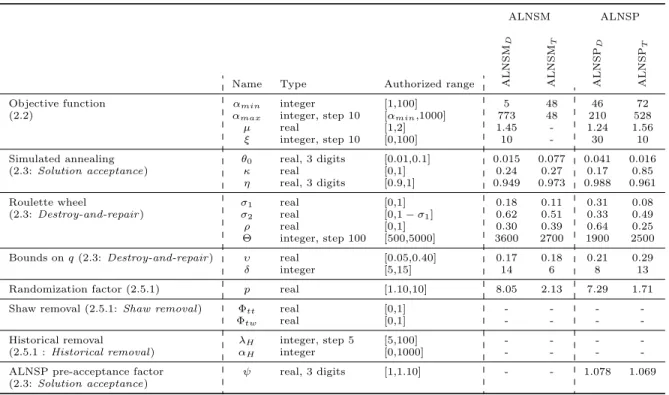
In Table 3, the type and range of numerical parameters (either real or integer) are specified, as well as their values in the four final configurations. Some of those parameters must be configured or not depending on the value taken by some others. For example, the weights used in version (a) of Shaw removal heuristic need to be configured only if the parameter corresponding to the use of this heuristic is TRUE. Unless otherwise specified, the configuration of real parameters is performed with a precision of two digits.

Table 3: Numerical parameter values in ALNSM and ALNSP configurations

ALNSM ALNSP

Name Type Authorized range ALNSM

D ALNSM T ALNSP D ALNSP T

Objective function αmin integer [1,100] 5 48 46 72

(2.2) αmax integer, step 10 [αmin,1000] 773 48 210 528

µ real [1,2] 1.45 - 1.24 1.56 ξ integer, step 10 [0,100] 10 - 30 10 Simulated annealing θ0 real, 3 digits [0.01,0.1] 0.015 0.077 0.041 0.016

(2.3: Solution acceptance) κ real [0,1] 0.24 0.27 0.17 0.85 η real, 3 digits [0.9,1] 0.949 0.973 0.988 0.961 Roulette wheel σ1 real [0,1] 0.18 0.11 0.31 0.08

(2.3: Destroy-and-repair ) σ2 real [0,1 − σ1] 0.62 0.51 0.33 0.49

ρ real [0,1] 0.30 0.39 0.64 0.25 Θ integer, step 100 [500,5000] 3600 2700 1900 2500 Bounds on q (2.3: Destroy-and-repair ) υ real [0.05,0.40] 0.17 0.18 0.21 0.29 δ integer [5,15] 14 6 8 13 Randomization factor (2.5.1) p real [1.10,10] 8.05 2.13 7.29 1.71 Shaw removal (2.5.1: Shaw removal ) Φtt real [0,1] - - -

-Φtw real [0,1] - - -

-Historical removal λH integer, step 5 [5,100] - - -

-(2.5.1 : Historical removal ) αH integer [0,1000] - - -

-ALNSP pre-acceptance factor ψ real, 3 digits [1,1.10] - - 1.078 1.069 (2.3: Solution acceptance)

3.2

Comparison with other Authors

We compare the results of our algorithms with those of the memetic algorithm of Cattaruzza et al. (2016a) and with the optimal solutions provided by the exact methods of Hernandez et al. (2016). For this purpose, we modify our objective function and minimize the total travel time instead of the total duration as explained in Section 3.1. The total travel time replaces the total duration in all the cost functions used to guide the search, including the criteria and cost functions of insertion and removal heuristics. Doing so, and setting the maximum allowed duration for each vehicle to the size of the planning horizon, we are able to provide a meaningful comparison with Cattaruzza et al. (2016a) on two sets of instances: those of Hernandez et al. (2016) and those of Cattaruzza et al. (2016a).

Hernandez et al. (2016) modify Solomon’s instances of groups C2, R2, and RC2, i.e., instances with large planning horizon. Travel times are calculated as Euclidean distances between each pair of

vertices, truncated to the first decimal place. Vehicle capacities are fixed to 100. The loading factor γ is equal to 0.2. Instances with 25 customers are generated by considering only the 25 first customers of Solomon’s graphs and 2 vehicles. Hernandez et al. (2016) provide optimal solutions for 25 out of those 27 instances with 25 customers. Hernandez et al. (2013) also report optimal results for 5 out of 27 instances similarly created with 50 customers and 4 vehicles. Cattaruzza et al. (2016a) extend this instance set by considering 27 instances, generated following the same methodology, with 100 customers and 8 vehicles. In the following, these instances are denoted by HFGN-25, HFGN-50, and HFGN-100, depending on the number of customers.

Cattaruzza et al. (2016a) also modify Solomon’s instances by introducing release dates and modifying the number of vehicles and their capacities considering travel times as Euclidean distances without rounding nor truncation. There is no loading time (γ = 0) and the vehicle capacity is set to half its original value. The fleet size is reported in Table 7, where we provide a comparison on the subset of their instances in which all release dates are equal to 0. In the following, these instances are denoted by CAF-100.

Thus, in total, we have 81 instances denoted HFGN-25, HFGN-50, and HFGN-100, involving respec-tively 25, 50, and 100 customers, and 56 instances denoted CAF-100 involving 100 customers.

The maximum run time is set to a time limit of 20, 50, and 250 seconds for instances with 25, 50, and 100 customers respectively for both configurations ALNSMT and ALNSPT. Tests are performed on

an Intel(R) Core(TM) i7-3930K CPU @ 3.20GHz. Cattaruzza et al. (2016a) use an Intel(R) Xeon(R) W3550 CPU @ 3.07GHz. Their maximum run time is set to 60 seconds for instances with 25 and 50 customers, and 300 seconds for instances with 100 customers.

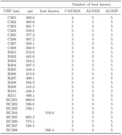
As shown in Table 4, both ALNSM and ALNSP produce the same solution value over five runs in all cases. This value is known to be optimal for 25 out of 27 instances. For the two instances that are not yet solved to optimality, the best known solution of Cattaruzza et al. (2016a) is reached.

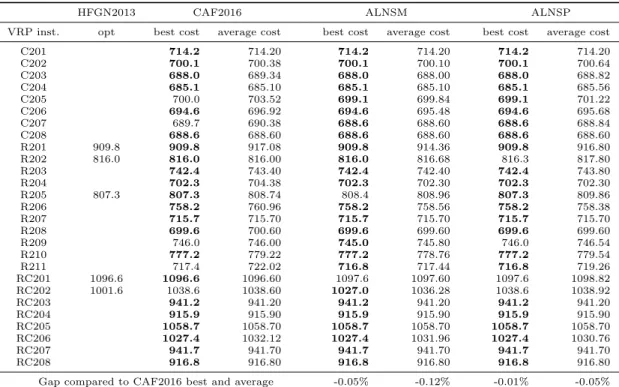
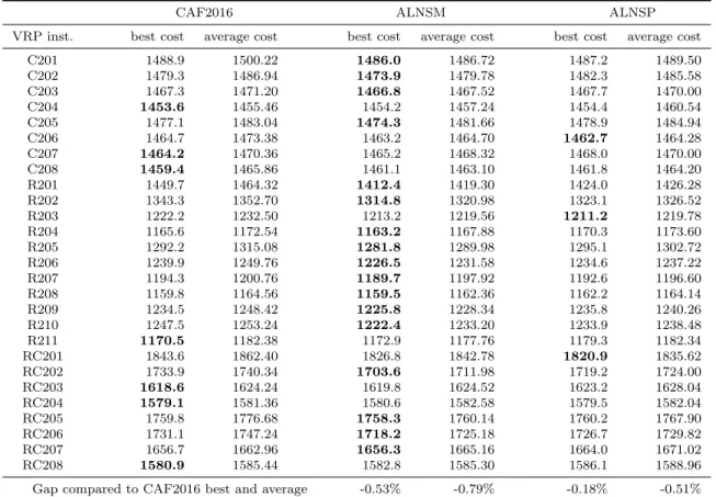
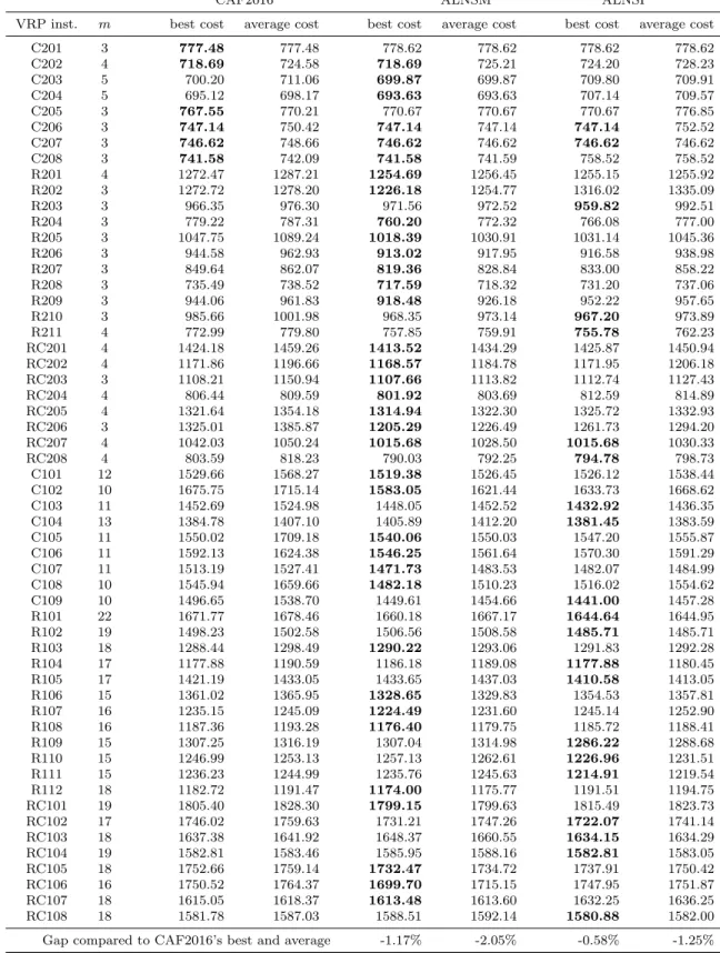
In Tables 5, 6, and 7, results of the ALNSM and ALNSP algorithms are compared with those of Cattaruzza et al. (2016a) on instance sets HFGN-50, HFGN-100, and CAF-100 respectively. For Table 5, the optimal value of Hernandez et al. (2013) is reported when known. The last row of each table contains a summarized comparison: the average percentage gap (over all instances) between the best ALNSM or ALNSP solution values and the best solution value of Cattaruzza et al. (2016a) is given, as well as the average percentage gap between the average ALNSM or ALNSP solution values over five runs and the average solution value of Cattaruzza et al. (2016a). Currently best known values are in bold. Both methods outperform the memetic algorithm of Cattaruzza et al. (2016a), with the ALNSM providing on average the best improvement.

Note that, for both algorithms, the post-optimization procedure only yields tiny improvements of the objective function value for a few instances. However, since it is extremely fast (less than one second for

Table 4: Results on HFGN-25 instances (n = 25, m = 2, γ = 0.2)

Number of best known VRP inst. opt best known CAF2016 ALNSM ALNSP

C201 380.8 4 5 5 C202 368.6 5 5 5 C203 361.7 5 5 5 C204 358.8 5 5 5 C205 377.2 5 5 5 C206 367.2 5 5 5 C207 359.1 5 5 5 C208 360.9 5 5 5 R201 554.6 5 5 5 R202 485.0 5 5 5 R203 444.2 5 5 5 R204 407.5 5 5 5 R205 448.4 5 5 5 R206 413.9 5 5 5 R207 400.1 5 5 5 R208 394.3 5 5 5 R209 418.3 5 5 5 R210 448.3 5 5 5 R211 400.1 5 5 5 RC201 660.0 5 5 5 RC202 596.8 5 5 5 RC203 530.1 5 5 5 RC204 518.0 5 5 5 RC205 605.3 5 5 5 RC206 575.1 4 5 5 RC207 528.2 5 5 5 RC208 506.4 5 5 5

Table 5: Results on HFGN-50 instances (n = 50, m = 4, γ = 0.2)

HFGN2013 CAF2016 ALNSM ALNSP

VRP inst. opt best cost average cost best cost average cost best cost average cost C201 714.2 714.20 714.2 714.20 714.2 714.20 C202 700.1 700.38 700.1 700.10 700.1 700.64 C203 688.0 689.34 688.0 688.00 688.0 688.82 C204 685.1 685.10 685.1 685.10 685.1 685.56 C205 700.0 703.52 699.1 699.84 699.1 701.22 C206 694.6 696.92 694.6 695.48 694.6 695.68 C207 689.7 690.38 688.6 688.60 688.6 688.84 C208 688.6 688.60 688.6 688.60 688.6 688.60 R201 909.8 909.8 917.08 909.8 914.36 909.8 916.80 R202 816.0 816.0 816.00 816.0 816.68 816.3 817.80 R203 742.4 743.40 742.4 742.40 742.4 743.80 R204 702.3 704.38 702.3 702.30 702.3 702.30 R205 807.3 807.3 808.74 808.4 808.96 807.3 809.86 R206 758.2 760.96 758.2 758.56 758.2 758.38 R207 715.7 715.70 715.7 715.70 715.7 715.70 R208 699.6 700.60 699.6 699.60 699.6 699.60 R209 746.0 746.00 745.0 745.80 746.0 746.54 R210 777.2 779.22 777.2 778.76 777.2 779.54 R211 717.4 722.02 716.8 717.44 716.8 719.26 RC201 1096.6 1096.6 1096.60 1097.6 1097.60 1097.6 1098.82 RC202 1001.6 1038.6 1038.60 1027.0 1036.28 1038.6 1038.92 RC203 941.2 941.20 941.2 941.20 941.2 941.20 RC204 915.9 915.90 915.9 915.90 915.9 915.90 RC205 1058.7 1058.70 1058.7 1058.70 1058.7 1058.70 RC206 1027.4 1032.12 1027.4 1031.96 1027.4 1030.76 RC207 941.7 941.70 941.7 941.70 941.7 941.70 RC208 916.8 916.80 916.8 916.80 916.8 916.80 Gap compared to CAF2016 best and average -0.05% -0.12% -0.01% -0.05%

Table 6: Results on HFGN-100 instances (n = 100, m = 8, γ = 0.2)

CAF2016 ALNSM ALNSP

VRP inst. best cost average cost best cost average cost best cost average cost

C201 1488.9 1500.22 1486.0 1486.72 1487.2 1489.50 C202 1479.3 1486.94 1473.9 1479.78 1482.3 1485.58 C203 1467.3 1471.20 1466.8 1467.52 1467.7 1470.00 C204 1453.6 1455.46 1454.2 1457.24 1454.4 1460.54 C205 1477.1 1483.04 1474.3 1481.66 1478.9 1484.94 C206 1464.7 1473.38 1463.2 1464.70 1462.7 1464.28 C207 1464.2 1470.36 1465.2 1468.32 1468.0 1470.00 C208 1459.4 1465.86 1461.1 1463.10 1461.8 1464.20 R201 1449.7 1464.32 1412.4 1419.30 1424.0 1426.28 R202 1343.3 1352.70 1314.8 1320.98 1323.1 1326.52 R203 1222.2 1232.50 1213.2 1219.56 1211.2 1219.78 R204 1165.6 1172.54 1163.2 1167.88 1170.3 1173.60 R205 1292.2 1315.08 1281.8 1289.98 1295.1 1302.72 R206 1239.9 1249.76 1226.5 1231.58 1234.6 1237.22 R207 1194.3 1200.76 1189.7 1197.92 1192.6 1196.60 R208 1159.8 1164.56 1159.5 1162.36 1162.2 1164.14 R209 1234.5 1248.42 1225.8 1228.34 1235.8 1240.26 R210 1247.5 1253.24 1222.4 1233.20 1233.9 1238.48 R211 1170.5 1182.38 1172.9 1177.76 1179.3 1182.34 RC201 1843.6 1862.40 1826.8 1842.78 1820.9 1835.62 RC202 1733.9 1740.34 1703.6 1711.98 1719.2 1724.00 RC203 1618.6 1624.24 1619.8 1624.52 1623.2 1628.04 RC204 1579.1 1581.36 1580.6 1582.58 1579.5 1582.04 RC205 1759.8 1776.68 1758.3 1760.14 1760.2 1767.90 RC206 1731.1 1747.24 1718.2 1725.18 1726.7 1729.82 RC207 1656.7 1662.96 1656.3 1665.16 1664.0 1671.02 RC208 1580.9 1585.44 1582.8 1585.30 1586.1 1588.96

Table 7: Results on CAF-100 instances (n = 100, γ = 0)

CAF2016 ALNSM ALNSP

VRP inst. m best cost average cost best cost average cost best cost average cost

C201 3 777.48 777.48 778.62 778.62 778.62 778.62 C202 4 718.69 724.58 718.69 725.21 724.20 728.23 C203 5 700.20 711.06 699.87 699.87 709.80 709.91 C204 5 695.12 698.17 693.63 693.63 707.14 709.57 C205 3 767.55 770.21 770.67 770.67 770.67 776.85 C206 3 747.14 750.42 747.14 747.14 747.14 752.52 C207 3 746.62 748.66 746.62 746.62 746.62 746.62 C208 3 741.58 742.09 741.58 741.59 758.52 758.52 R201 4 1272.47 1287.21 1254.69 1256.45 1255.15 1255.92 R202 3 1272.72 1278.20 1226.18 1254.77 1316.02 1335.09 R203 3 966.35 976.30 971.56 972.52 959.82 992.51 R204 3 779.22 787.31 760.20 772.32 766.08 777.00 R205 3 1047.75 1089.24 1018.39 1030.91 1031.14 1045.36 R206 3 944.58 962.93 913.02 917.95 916.58 938.98 R207 3 849.64 862.07 819.36 828.84 833.00 858.22 R208 3 735.49 738.52 717.59 718.32 731.20 737.06 R209 3 944.06 961.83 918.48 926.18 952.22 957.65 R210 3 985.66 1001.98 968.35 973.14 967.20 973.89 R211 4 772.99 779.80 757.85 759.91 755.78 762.23 RC201 4 1424.18 1459.26 1413.52 1434.29 1425.87 1450.94 RC202 4 1171.86 1196.66 1168.57 1184.78 1171.95 1206.18 RC203 3 1108.21 1150.94 1107.66 1113.82 1112.74 1127.43 RC204 4 806.44 809.59 801.92 803.69 812.59 814.89 RC205 4 1321.64 1354.18 1314.94 1322.30 1325.72 1332.93 RC206 3 1325.01 1385.87 1205.29 1226.49 1261.73 1294.20 RC207 4 1042.03 1050.24 1015.68 1028.50 1015.68 1030.33 RC208 4 803.59 818.23 790.03 792.25 794.78 798.73 C101 12 1529.66 1568.27 1519.38 1526.45 1526.12 1538.44 C102 10 1675.75 1715.14 1583.05 1621.44 1633.73 1668.62 C103 11 1452.69 1524.98 1448.05 1452.52 1432.92 1436.35 C104 13 1384.78 1407.10 1405.89 1412.20 1381.45 1383.59 C105 11 1550.02 1709.18 1540.06 1550.03 1547.20 1555.87 C106 11 1592.13 1624.38 1546.25 1561.64 1570.30 1591.29 C107 11 1513.19 1527.41 1471.73 1483.53 1482.07 1484.99 C108 10 1545.94 1659.66 1482.18 1510.23 1516.02 1554.62 C109 10 1496.65 1538.70 1449.61 1454.66 1441.00 1457.28 R101 22 1671.77 1678.46 1660.18 1667.17 1644.64 1644.95 R102 19 1498.23 1502.58 1506.56 1508.58 1485.71 1485.71 R103 18 1288.44 1298.49 1290.22 1293.06 1291.83 1292.28 R104 17 1177.88 1190.59 1186.18 1189.08 1177.88 1180.45 R105 17 1421.19 1433.05 1433.65 1437.03 1410.58 1413.05 R106 15 1361.02 1365.95 1328.65 1329.83 1354.53 1357.81 R107 16 1235.15 1245.09 1224.49 1231.60 1245.14 1252.90 R108 16 1187.36 1193.28 1176.40 1179.75 1185.72 1188.41 R109 15 1307.25 1316.19 1307.04 1314.98 1286.22 1288.68 R110 15 1246.99 1253.13 1257.13 1262.61 1226.96 1231.51 R111 15 1236.23 1244.99 1235.76 1245.63 1214.91 1219.54 R112 18 1182.72 1191.47 1174.00 1175.77 1191.51 1194.75 RC101 19 1805.40 1828.30 1799.15 1799.63 1815.49 1823.73 RC102 17 1746.02 1759.63 1731.21 1747.26 1722.07 1741.14 RC103 18 1637.38 1641.92 1648.37 1660.55 1634.15 1634.29 RC104 19 1582.81 1583.46 1585.95 1588.16 1582.81 1583.05 RC105 18 1752.66 1759.14 1732.47 1734.72 1737.91 1750.42 RC106 16 1750.52 1764.37 1699.70 1715.15 1747.95 1751.87 RC107 18 1615.05 1618.37 1613.48 1613.60 1632.25 1636.25 RC108 18 1581.78 1587.03 1588.51 1592.14 1580.88 1582.00

3.3

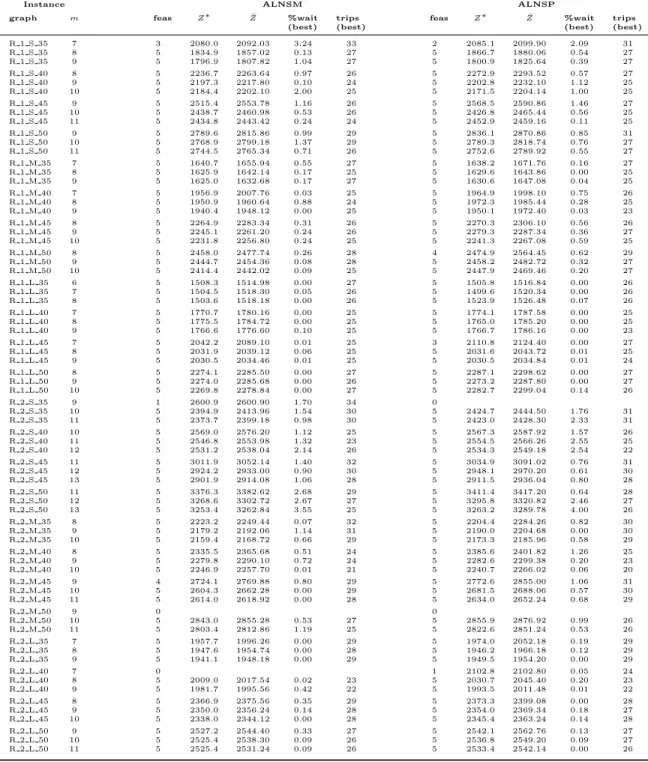
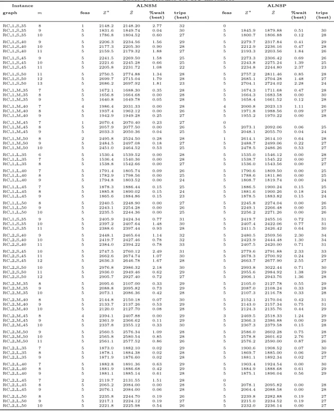
Results for New MTVRPTW Instances

Creating suitable instances, where multiple trips naturally arise, by modifying Solomon’s instances is not a straightforward task, especially when the maximum allowed duration per vehicle is shorter than the planning horizon. Indeed, multiple trips are favored by decreasing the vehicle capacities, implying an increase in the number of vehicles to be used. The fleet size has to be increased even more when the allowed duration for each vehicle is shortened, but this decreases the necessity to create multiple trips. Let us consider CAF-100 instances of groups R1 and RC1. For these instance groups, Cattaruzza et al. (2016a) use a number of vehicles ranging from 15 to 22. For most instances of Table 7, the number of trips obtained in the solution is nearly the same as the number of vehicles. Logically, if the maximum allowed duration per vehicle is shortened, and the fleet size consequently increased for each instance, then each vehicle will serve very few customers, often even only one or two per trip, and the number of trips per vehicle will tend to decrease.

For these reasons, we create a new set of instances with 100 customers that we believe have suitable characteristics for MTVRPTW variants. We follow the general philosophy of Solomon by dividing our instances into three groups of geographical customer repartitions (clustered (C), random (R), and random clustered (RC)) and two planning horizon sizes (short (1) with size 600 and long (2) with size 1200), while the maximum allowed duration per vehicle Dmax is 480 in all cases.

For each of the six resulting groups, we generate four different instance bases. Each basis is defined by the geographical coordinates of the customers and the depot, as well as the customer demands, time window centers, and service times. For each of the 24 obtained instance bases, three sizes of time windows are considered: large (L), with size 240, medium (M ), with size 120, and small (S), with size 60. The combination of the 24 initial instance bases with three time window sizes results in 72 instance graphs. Each of these is coupled with three values of m to create the final set of instances. For all instances, the vehicle capacity is fixed at 100 and the loading factor is 0.2.

The names of the 72 instance graphs begin with the geographical type, followed by the size of the planning horizon and the time window size. For example, graph names beginning with R 1 M indicate a random geographical repartition of the customers, a small planning horizon, and medium time windows. The values of m chosen for each one of the 72 graphs are respectively the minimum value of m for which we were able to obtain a feasible solution, v, along with v + 1 and v + 2. For example, if for a given instance graph, solution values are reported for m ∈ {7, 8, 9}, then it means that we could not find any feasible solution for m = 6 on the same instance graph. Five graphs that could not be solved using less than 15 vehicles have been discarded, since we try to mimic a realistic multi-trip context. This leads to a final set of 201 MTVRPTW instances.

The numerical parameters of the instances and the methods employed to generate customer clusters, time windows, and demands are detailed in the Appendix. The instance files, and the Julia notebook