Next-Point Prediction for Direct Touch Using Finite-Time Derivative Estimation

(1)

HAL Id: hal-01893310

https://hal.inria.fr/hal-01893310

Submitted on 11 Oct 2018

HAL is a multi-disciplinary open access

archive for the deposit and dissemination of

sci-entific research documents, whether they are

pub-lished or not. The documents may come from

teaching and research institutions in France or

abroad, or from public or private research centers.

L’archive ouverte pluridisciplinaire HAL, est

destinée au dépôt et à la diffusion de documents

scientifiques de niveau recherche, publiés ou non,

émanant des établissements d’enseignement et de

recherche français ou étrangers, des laboratoires

publics ou privés.

Next-Point Prediction for Direct Touch Using

Finite-Time Derivative Estimation

Mathieu Nancel, Stanislav Aranovskiy, Rosane Ushirobira, Denis Efimov,

Sébastien Poulmane, Nicolas Roussel, Géry Casiez

To cite this version:

Mathieu Nancel, Stanislav Aranovskiy, Rosane Ushirobira, Denis Efimov, Sébastien Poulmane, et

al.. Next-Point Prediction for Direct Touch Using Finite-Time Derivative Estimation. Proceedings

of the ACM Symposium on User Interface Software and Technology (UIST 2018), Oct 2018, Berlin,

Germany. �10.1145/3242587.3242646�. �hal-01893310�

(2)

Next-Point Prediction for Direct Touch

Using Finite-Time Derivative Estimation

Mathieu Nancel

1,2

_{Stanislav Aranovskiy}

3

_{Rosane Ushirobira}

1,2

_{Denis Efimov}

1,2

S´ebastien Poulmane

1,2

_{Nicolas Roussel}

1,2

_{G´ery Casiez}

2,1 1

_{Inria, France}

2

_{Univ. Lille, UMR 9189 - CRIStAL, Lille, France}

3

_{IETR, CentraleSupelec, Rennes, France}

ABSTRACT

End-to-end latency in interactive systems is detrimental to performance and usability, and comes from a combination of hardware and software delays. While these delays are steadily addressed by hardware and software improvements, it is at a decelerating pace. In parallel, short-term input pre-diction has shown promising results in recent years, in both research and industry, as an addition to these efforts. We describe a new prediction algorithm for direct touch devices based on (i) a state-of-the-art finite-time derivative estimator, (ii) a smoothing mechanism based on input speed, and (iii) a post-filtering of the prediction in two steps. Using both a pre-existing dataset of touch input as benchmark, and subjective data from a new user study, we show that this new predictor outperforms the predictors currently available in the literature and industry, based on metrics that model user-defined nega-tive side-effects caused by input prediction. In particular, we show that our predictor can predict up to 2 or 3 times further than existing techniques with minimal negative side-effects.

Author Keywords

touch input; latency; lag; prediction technique.

INTRODUCTION

End-to-end latency in interactive systems is the sum of all hardware and software delays (e.g. sensing, recognition, stored memory, rendering) between a physical input and the displaying of its effects (e.g. respectively a key press and the appearance of the corresponding letter on screen).

Current direct touch systems present end-to-end latencies ranging from 50 to 280 ms [3, 22]. These values are above perception thresholds and degrade performance. Previous studies have shown that users can notice end-to-end laten-cies as low as 2 ms with a pen [21] and 5 to 10 ms with a finger [22]. Performance is degraded from 25 ms in dragging tasks with a finger [12]. Deber et al. further show that im-provements in latency as small as 8 ms are noticeable from a wide range of baseline latencies [12]. While we can expect

Permission to make digital or hard copies of all or part of this work for personal or classroom use is granted without fee provided that copies are not made or distributed for profit or commercial advantage and that copies bear this notice and the full cita-tion on the first page. Copyrights for components of this work owned by others than ACM must be honored. Abstracting with credit is permitted. To copy otherwise, or re-publish, to post on servers or to redistribute to lists, requires prior specific permission

and/or a fee. Request permissions fromPermissions@acm.org.

UIST 2018, October 14–17, 2018, Berlin, Germany c 2018 Association for Computing Machinery. ACM ISBN 978-1-4503-5948-1/18/10. . . $15.00 https://doi.org/10.1145/3242587.3242646

that next generations of touch interactive systems will exhibit less latency using, for example, higher frequency input and output, this comes at the cost of higher power consumption and its complete suppression seems unlikely.

In combination with latency reduction, latency compensation using next-point prediction techniques offers a promising av-enue to cope with latency. In dragging tasks, these techniques use previous touch positions to predict the next ones in a near future in order to estimate the current finger position [20]. The existing prediction techniques are mainly based on Tay-lor series [5, 17, 25, 28, 29], Kalman filters [14, 16, 18, 26, 27], curve fitting [1], heuristic approaches [13], and neural net-works [10, 11]. Only a few of them have been evalu-ated [5,10]. Nancel et al. have shown that input prediction in-troduces noticeable side-effects such as jitter or spring-effect. They characterized and proposed metrics to measure these side-effects [20]. They report that participants perceived la-tency as less disturbing than the side-effects introduced by current prediction techniques when trying to fully compen-sate latency. As a result, next-point prediction techniques can only be useful if they can compensate some of the latency while minimizing the side-effects they introduce.

We contribute a new prediction algorithm for direct touch de-vices designed to offer good trade-offs between latency re-duction and side-effects. It is based on a state-of-the-art, finite-time differentiator that provides estimation of the first, second and third time derivatives of the input position in a predefined, limited time. It is combined with a smoothing mechanism that dampens the amplitude of the prediction de-pending on the user’s input speed, to minimize jitter [4, 20]. Using a pre-existing large dataset of touch input as bench-mark, we show that this new predictor outperforms the pre-dictors currently available in the literature and industry for direct touch input, based on metrics that model user-defined negative side-effects caused by input prediction. These re-sults were then confirmed in a controlled user experiment.

(3)

The paper makes the following contributions:

• the introduction of the HOM finite-time derivative estima-tor to the HCI community, to go beyond computing deriva-tives limited to straightforward calculations,

• the adaptation of HOM to include a speed-based smoothing mechanism, and its first application to latency compensa-tion with direct touch,

• the design and application of an optimization algorithm for the parameters of a HOM-based input predictor that can be adapted to system and user requirements,

• the validation of a stroke dataset from the literature to serve as benchmark for new predictors (in appendix),

• the formulation of a unique metric for the benchmarking of input prediction algorithms,

• an extensive, simulation-based validation of the resulting technique against state-of-the-art input predictors,

• a user experiment providing subjective comparison of our prediction technique against state of the art predictors, for different tasks and levels of compensation.

After addressing the related work we describe our prediction technique before detailing its evaluation.

RELATED WORK

Our review of the related work first covers measures and human factors related to end-to-end latency on direct touch surfaces before detailing current next-point prediction tech-niques and time derivative estimation methods.

End-to-end Latency in Direct Touch

In 2012 Ng et al. measured latency on various touch de-vices and found end-to-end latencies ranging from 60 to 200 ms [22]. More recently Casiez et al. found end-to-end la-tency on current touch devices ranging from 48 to 276 ms and show it is affected by the hardware, operating system and toolkit [3]. The authors further show that the input latency (time from a physical action of the user on an input device to the reception of the corresponding event by the system) is in the range 14 to 25 ms using native toolkits on Android devices and that most of the end-to-end latency comes from the output latency (time elapsed between calling the repaint of the display and its actual update) which is affected by the operating system, graphic card and physical screen.

The impact of end-to-end latency on user perception and per-formance in direct touch interaction is well covered in the lit-erature. For dragging tasks, users can reliably perceive touch-screen latency as low as 5-10 ms [22] as they can easily notice the physical distance between their finger and the associated visual stimulus [6]. For tapping tasks, the perception thresh-old is higher at 24 ms [12]. The threshthresh-olds are even lower using a pen. Ng et al. reported 2 ms for dragging and 6 ms for scribbling [21]. Jota et al. showed that performance is affected from 25 ms in dragging tasks with a finger [12]. To sum up, current systems show latencies above perception and performance thresholds. Ideally even the most efficient systems showing 50 ms latency should reduce their latency

by 25 ms to prevent human performance degradation, and by 40 ms to make the latency un-noticeable. Deber et al. have also shown that improvements in latency as small as 8 ms are noticeable from a wide range of baseline latencies [12]. If one can expect current hardware will improve in a near future to reduce latency, its complete suppression is unlikely.

Next-point Prediction Techniques

Nancel et al. [20] detailed existing related work on next-point prediction techniques that fall into four main categories: Tay-lor series [5, 17, 25, 28, 29], Kalman filter [14, 16, 18, 26, 27], curve fitting [1] and heuristic approaches [13]. See Nancel et al. for a detailed description of these techniques [20]. More recently Henze et al. used neural networks for prediction and found their technique to be more precise than first-, second-and third-order polynomial extrapolations [10,11]. Their neu-ral networks were trained on a very large data collection. We could unfortunately not integrate this technique in our study, as the data and code to train new networks to our experiment’s latencies and device were not available at the time. The ap-proach in [11] and the one presented in this article thus remain to be compared.

If current next-point prediction techniques can compensate some of the latency, they also introduce prediction artifacts. Nancel et al. characterized the side-effects introduced by these techniques and noticed by participants and classified them in 7 categories: lateness, over-anticipate, wrong dis-tance, wrong orientation, jitter, jumps, and spring effect [20]. In addition they developed quantitative metrics that correlate positively with the frequency of perceived side-effects. With the exception of the curve fitting and neural networks techniques, all other techniques rely on the use of speed and acceleration determined from the finger positions. These derivatives are estimated using simple time differentiation based on the two previously acquired positions or computed speeds. Simple time differentiation techniques have the bene-fit of being straightforward to implement and fast to execute. Furthermore they use the most recent information available and thus introduce a small latency in the estimation of speed or acceleration. However the resulting computation of speed and acceleration are generally noisy, which results in higher chances to notice side-effects. Yet, more advanced techniques to estimate derivatives also exist.

Time Derivative Estimation Techniques

Numerical differentiation is a key issue in the domains of sig-nal processing and control engineering as it appears in many problems where a noisy signal needs to be reconstructed or filtered. There are many methods providing numerical dif-ferentiation with different levels of performance (the most important of them being sensitivity to measurement noises, computational complexity, and estimation delay). Popular techniques include statistical approaches such as the mini-mum least squares method [7]. In recent years, novel deter-ministic approaches have been proposed yielding good results in terms of robustness to noise and computational aspects. In this framework, we may cite the approach based on the sliding mode methods [8, 15], algebraic methods [9, 24] or

(4)

the homogeneous systems method [19, 23]. Minimum least squares and sliding mode approaches either have to be com-puted off-line, or present significant chattering, defined as an undesirable phenomenon of oscillations with finite frequency and amplitude. Algebraic methods are robust to noise but introduce some delay in the estimations. The homogeneous-based differentiator has a fast rate of convergence and good robustness with respect to disturbances. It appears as the most appropriate numerical differentiation technique in the context of latency compensation. In the following we refer to this technique as ‘HOM’, short for homogeneous.

We clarify that the HOM finite-time derivative estimator is not a next-point prediction algorithm. It is a general-purpose method introduced in 2008 [23], initially to secure communi-cations. This paper is highly cited in the control theory com-munity, showing the method’s applicability in various con-texts, but never for latency compensation until 2016 [24]. In [24], the HOM differentiator was compared to other differ-entiators for basic latency compensation with a mouse. How-ever that involved minimal validation, using small datasets and simplistic metrics based on predicted-to-actual distances; such metrics were later shown to be limited and possibly mis-leading [20]. Therefore the results in [24] remain to be con-firmed, especially for direct touch for which latency can be more noticeable than with a mouse. HOM has never been used for latency compensation with direct touch. In fact, de-spite its 10 years of existence it was never brought to the HCI literature, in which the typical method to compute derivatives remains mostly limited to straightforward calculations of the form (pi pi 1)/(ti ti 1)relative to the last input event i,

where piis the value of the signal at the instant ti.

Another approach based on finite impulse response (FIR) fil-ters has been proposed recently in [2]. It demonstrates good robustness properties with respect to measurement noise, but still requires more computational capacities (involves matrix manipulations with 16 times 16 matrices for both X and Y) without a corresponding quality of differentiation improve-ment comparing to HOM differentiator. In addition the FIR has at least 16 tunable gains for each axis, against 5 for HOM.

THE TURBOTOUCH PREDICTOR

Given a measured position1_x

m(tk)at a time tk, the TURBO

-TOUCHpredictor (TTp) algorithm2attempts to estimate a real

object’s position x(tk)using features of the ongoing

trajec-tory. The measured position is always sensed with a certain latency L: _x_m_(t_k) =x(tk L)

In practice the value L is not constant, but for algorithm design and performance evaluation purposes we impose the assumption that an averaged constant value L0 is available.

Therefore, we can define the estimation error e(tk)between

the real position x(tk)and its estimate ˆx(tk):

e(tk) =x(tk) ˆx(tk)⇡ xm(tk+L0) ˆx(tk)

1_{The calculations that follow are described for the x coordinate only}

for simplicity, and must be performed for y as well in real use.

2_{Our prediction algorithm and tuning process are available at}

ns.inria.fr/loki/TTp/.

The approximate equality becomes exact assuming L0=L, in

such a case the error between the real position x(tk)and the

estimate ˆx(tk) is exactly the difference between the further

measured position xm(tk+L0)and the estimate ˆx(tk).

Perhaps intuitively, there exists a trade-off between high-frequency oscillations of the predicted cursor, or “jitter”, and how promptly a predicted cursor reacts to quick changes in trajectory or in speed. This trade-off is more noticeable when large amounts of latency need to be compensated. Nancel et al. [20] reported that:

• estimators that use only the most recent measured posi-tions tend to react faster to input change, but increase the chances of cursor jitter. Using points further away in the past lowers the risk of jitter, but delays the cursor’s re-sponse to sudden changes of input speed and direction, • participants’ reports of jitter were negatively correlated

with reports of “lateness” of the cursor, from which we infer that compensating smaller amounts of latency lowers the risks of noticeable jitter, but increase the noticeable lag, • participants reported more jittery cursor movements when moving slowly. No correlation was observed between slow movements and reported “lateness”, but it is trivial to cal-culate that, for a constant latency, lower speeds result in smaller—and therefore less noticeable—offsets.

To summarize, when most of the latency is to be compen-sated, estimations calculated from most “recent” measures react faster to sudden changes of trajectory, but increase the chances of jitter. Jitter, however, is more noticeable when the user is moving slowly.

To cope with the aforementioned trade-off, the main fea-ture of the proposed design is that the prediction is smoothly turned off when the instant velocity of the controlled object, further denoted as V (t), is sufficiently low. This simultane-ously limits jitter with admissibly small prediction error for low velocities, and provides fast cursor reactions for medium and high velocities.

The proposed estimator behaves according to the following rules, where Vlowis a general parameter.

• If V (tk) Vlow, then the predictor behaves normally by

ex-trapolating from the most recent features of the trajectory. • If V (tk) <Vlow, then the main goal of the estimator is to

avoid any noise amplification, and a good strategy is to turn off estimation and bypass the measurements.

• To avoid discontinuities (jumps) in estimation, the switch-ing is smoothed with an exponential weightswitch-ing function. • Finally, to remove any remaining noise in the predicted

po-sitions, we apply a light filtering using the 1e filter [4].

Estimator Description

We use the estimator

ˆx(tk) =xm(tk) +a(tk) ⇣ ˆf> x (tk)· qx ⌘ (1)

(5)

where ˆf>

x (tk)· qx is the estimation of the input movement

since the most recently measured position xm(tk). It is

com-posed of an estimate of the vector of time derivatives fx(tk):= [x(1)m (tk),x(2)m (tk),x(3)m (tk)]>

and a constant gain vectorqx2 R4obtained by off-line

opti-mization (see below).a(tk)2 R+is the exponential

weight-ing function that implements the smoothweight-ing mentioned above. The estimate ˆfx(tk)is computed using HOM [23].

sx(tk) =HOM(sx(tk 1),xm(tk),ax,lx,Dt) ,

ˆfx(tk) = [sx,2(tk),sx,3(tk),sx,4(tk)]>, (2)

where sx(tk)is the state vector of the differentiator,ax>0 and

lx2 [ 0.2,0] are the differentiator’s parameters obtained by

off-line optimization (see below) , andDt is the integration

interval, a general parameter. The HOM is a discrete-time approximation of the continuous-time differential equation

The exponential weighting functiona(tk)above is computed

as a(tk) =a(tk 1) +ga(a?(tk) a(tk 1)) (4)

with 0 <ga<1 a general parameter and a?_(t

k) =

⇢₁ _{if V (t}

k) Vlow,

0 if V (tk) <Vlow. (5)

The estimator’s constant gain vectorqxis obtained via off-line

minimization of the estimation cost function defined below. Readers will have noted that neither the actual latency L nor the expected average latency L0appear in the computations

above. This is because L0is a parameter of the training

pro-cess in which the values ofax,lx, andqxare optimized (see

below). These values therefore correspond to a specific input-output setup (from which the training data is gathered) as well as a specific amount of latency compensation. Compensating for a new latency therefore requires to run a new optimization. Note also that the parameters ax, lx and qx are obtained

through an optimization process whose main purpose is to minimize metrics of prediction error, not to estimate speed, acceleration, and jerk as closely as possible to physical units. For that reason, the estimates ˙sx,n(tk) need to be remapped

to physical scales before they can be used as estimations of speed, acceleration, or jerk, e.g. in Eq. 5: Vx(tk) =

µ ⇥ sx,2(tk). The parameter µ is obtained through off-line

optimization (see below).

Switched Estimator Algorithm

We now describe every step of a typical, real-time use of our switched estimator algorithm. For the sake of simplicity and understanding the algorithm is described in a 2D context but

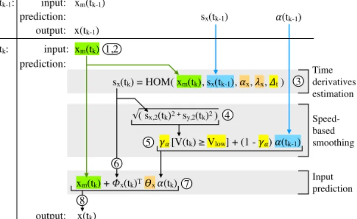
xm(tk) sx(tk-1) !(tk-1) sx(tk) = HOM( xm(tk), sx(tk-1), !x, "x, #t ) $! [V(tk) ≥ Vlow] + (1 - $!) !(tk-1) xm(tk) + %x(tk)T &x !(tk) tk: tk-1: xm(tk-1) x(tk-1) input: output: input: output: x(tk) Time derivatives estimation Speed-based smoothing Input prediction 1,2 3 4 5 6 7 8 prediction: prediction: √( sx,2(tk)2 + sy,2(tk)2 )

Figure 1: General description of real-time prediction process, with step numbers. Input in green, previously computed variables in blue, general parameters in yellow, optimized parameters in orange.

could be easily extended in 3D. It can also be adapted for rotations or any other input channel used for pointing. Input signals. At each step the input signals are the time in-stance tkand the measurements xm(tk), ym(tk).

Output signals. At each step the output signals are the estima-tions ˆx(tk), ˆy(tk).

Parameters. The estimator has the following parameters: • the HOM parameters:

ax,ay > 0,

lx,ly 2 [ 0.2,0],

Dt > 0 (integration time step)

• the gains qx,qy2 R3,

• the HOM conversion ratio µ, • the velocity threshold Vlow 0,

• the smoothing parameter 0 < ga<1.

Internal variables. The internal variables of the estimator are the timer variablet 2 R, the differentiator states sx,sy2 R5,

and the weighting variablea 2 R.

Initialization. At the first time instance t1set

t = t1, sx(t1) = [xm(t1),0, 0, 0, 0]>, sy(t1) = [ym(t1),0, 0, 0, 0]>, a(t1) =0, ˆx(t1) =xm(t1), ˆy(t1) =ym(t1).

Estimation. At each time instance tk, k > 1:

Step 1. Get the new measurements.

Step 2. Pre-process the measurements. This step includes: input data verification, units conversion and time frames adjustment between the estimator and the

(6)

measurements provider. The output of this step are the preprocessed values tk, xm(tk)and ym(tk).

Step 3. Update the internal variable t and the states sx(tk),

sy(tk)as follows:

(a) Set sx(tk) =sx(tk 1)and sy(tk) =sy(tk 1).

(b) Whilet < tk, repeat:

i. Compute ex(tk) = sx,1(tk) xm(tk) and

ey(tk) =sy,1(tk) ym(tk), where sx,i and sy,i

are the i-th elements of the vectors sxand sy,

sy,3(tk) 10ay2|ey(tk)|1+2lysign(ey(tk))

sy,4(tk) 10ay3|ey(tk)|1+3lysign(ey(tk))

sy,5(tk) 5ay4|ey(tk)|1+4lysign(ey(tk)) a5 y|ey(tk)|1+5lysign(ey(tk)) 3 7 7 7 7 5Dt iii. Updatet = t + Dt.

Step 4. Compute the estimate of 2D velocity absolute value ˆV(tk) =µ q (sx,2(tk))2+ (sy,2(tk))2, anda?_as a?_(t k) = ⇢₁ _{if V (t} k) >Vlow, 0 if V (tk) Vlow.

Step 5. Update the internal variablea as

a(tk) =a(tk 1) +ga(a?(tk) a(tk 1)) .

Step 6. Define the estimates of derivatives

ˆfx(tk) = [sx,2(tk),sx,3(tk),sx,4(tk)]>,

ˆfy(tk) = [sy,2(tk),sy,3(tk),sy,4(tk)]>.

Step 7. Compute the estimates

ˆx(tk) =xm(tk) +a(tk) ˆfx>(tk)qx,

ˆy(tk) =ym(tk) +a(tk) ˆfy>(tk)qy.

Step 8. Post-process the estimates. This step includes units conversion and time frames adjustment between the estimator and an output device.

Implemented in C++, the above algorithm results in about 150 lines of code without the use of any external function. One prediction takes 1.5µs on average (95th _{percentile = 2}

µs, max = 44 µs) on an i7 4GHz processor, a few orders of magnitude below the amount of latency considered.

Parameters Tuning

The parameters used in the algorithm can be divided into two groups: the general parameters and the optimization-based parameters. The general parameters are tuned manu-ally, taking into account physical and hardware specifications of the exact estimation problem and input/output devices. The optimization-based parameters are tuned using a given dataset of movements specific to the considered estimation problem, minimizing metrics described below.

General Parameters

The general parameters used at runtime are the integration in-tervalDt>0 and the parameters of the speed-based

smooth-ing: the velocity threshold Vlow 0 and the smoothing gain

ga 2]0,1[. Vlow depends on visual tolerance, ga on

behav-ior change tolerance, andDton computational capabilities, as

detailed below.

• Dt is less or equal to the measurement period Ts. This

value is a trade-off between computational time and ac-curacy, and depends on the target hardware. It is typically expressed as a proportion p of the system’s average sam-pling period: Dt =p.Ts. For example, in our benchmark

below we use the whole period (p = 1) on a sampling fre-quency of 120 Hz, soDt=1 ⇥ 1000/120 = 8.33 ms.

• Vlowdefines the minimum velocity at which the estimator

is activated. It corresponds to the input speed below which the system latency is considered not noticeable; in our case, when the visual lag is hidden under the finger. The general idea is to switch the estimator on at a velocity for which the lag becomes noticeable to most users. The following formula is proposed for its adjustment:

Vlow=Emax

L0 ,

where Emax is the maximal admissible error in distance

units. For example, if we assume that the end-to-end la-tency is 68 ms and a typical user is affected by a deviation greater than 7 mm (as an estimation of finger radius), then a reasonable choice would be Vlow=7mm_68ms⇡ 100 mm/s. The

value of Vlowmay be updated given users feedback.

• 0 < ga<1 defines the exponential smoothing transient de-cay time, _g

a=1 0.05ttransientsTs _,

where ttransientsis the admissible transient time of switching

between two modes of the estimator. Assuming a desired transient time of 0.33 ms with 120 Hz sampling frequency, the corresponding value ofgais computed as

ga=1 0.058.33ms0.33s _{⇡ 0.73.}

These rule-of-thumb formulae define initial values for our general parameters and we found them to work well in prac-tice. These parameters could benefit from empirical tuning or extended exploration of their range and effects, but this is left to future work.

Two other general parameters are used in the optimization of the other predictor’s parameters (see below):

(7)

• The expected average lag value L0. The shifted

measure-ments xm(tk+L0)are further used to optimize the

estima-tor’s parameters.

• The jitter lower frequency bound Fbis the oscillation

fre-quency above which cursor movements are interpreted as undesirable jitter. Along with Fb we consider HFGlow

and HFGhigh, the jitter amplification levels considered as

“low” and “high”, see below for the details on amplifica-tion level computaamplifica-tion procedure. Based on our experi-ments these values are chosen as Fb=7Hz, HFGlow=5

and HFGhigh=6.

Optimized Parameters

The parameters tuned via optimization are the time differ-ential gainsqx,qy2 R3, the HOM conversion ratioµ, and

the HOM differentiator parametersax,ay2 R+andlx,ly2

[ 0.2,0]. Note that HOM has been used in very different domains, and many application-related methods have been developed to tune its parameters. Our tuning protocol fol-lows the general principles of these existing methods, but is adapted to the specific problem of latency compensation. The estimation algorithm considers each axis separately, so the corresponding parameters are optimized separately as well. However, the tuning procedure is the same. Below we describe the tuning procedure for the x axis only.

The input data set D consists of equally spread time instances tkand the corresponding measurements xm(tk), k = 1,...,N.

For the tuning procedure it is assumed that a sufficiently large data set is available representing all kinds of possible / admis-sible movements.

Metrics used

• The high-frequency gain HFG( ˆx) represents how the esti-mator amplifies the input oscillation frequencies above Fb

with respect to the measured position. We compute this value as follows. First, using fast Fourier transform (e.g. Matlab’s fft function) we remove from the signals ˆx and xm all the components below the frequency Fb. Then, the

ratio of the L1 norms of the filtered signals is computed

and considered as the noise amplification level. • The mean average estimation error is computed as

E1(ˆx) = 1 N N0 N N0

Â

i=1 |xm (ti+L0) ˆx(ti)|,

where N0 is the maximum integer below L_T0_s, i.e. latency

value expressed in number of sampling intervals. The mean average error with respect to no estimation, is fur-ther denoted as E10=_{N N}1 0 N N0

Â

i=1 |x m(ti+L0) xm(ti)|.

• The maximum estimation error is computed as E•(ˆx) = max

i |xm(ti+L0) ˆx(ti)|.

The maximum error with respect to no estimation, is fur-ther denoted as

E•0=max_i |xm(ti+L0) xm(ti)|.

• The cost function J( ˆx) of the estimation is computed as J( ˆx) =k1J1(ˆx) +k2J2(ˆx) +k3J3(ˆx),

wherek1>0,k2>0 andk3>0 are tunning constants and

J1(ˆx) = E1(ˆx) E0 1 , J2(ˆx) = E•_E(ˆx)₀ • , J3(ˆx) = 8 > < > : 0 if HFGhigh HFG( ˆx) HFG( ˆx) HFGlow

HFG_high HFG_low if HFGlow<HFG( ˆx) < HFGhigh

1 if HFG( ˆx)  HFGlow

In our experiments we havek1=k2=k3=1. However,

these values can be modified given user experience feed-back.

Parameter tuning

With the above, for any given estimate ˆx we can compute the performance index J( ˆx). Our goal is to find values for the parametersax,lx, andqxthat produce predictions that

mini-mize this performance index over the given dataset D. Recall that the parametersaxandlxare used to compute the output

ˆfxof the HOM differentiator (2), so we can write

ˆfx(tk) = ˆfx(tk|ax,lx) ,

andqxis used to compute the estimate ˆx, see (1),

ˆx(tk|ax,lx,qx) =xm(tk) +a(tk) ˆfx>(tk|ax,lx)qx.

We therefore use two optimization loops. The inner loop con-sidersaxandlxas input parameters and attempts to find the

bestqxfor the given dataset D and HOM output ˆfx(tk|ax,lx).

The output of this inner loop is defined as Jinner(ax,lx), the

lowest cost function score for the chosenaxandlx. The

sec-ond, outer loop searches foraxandlxusing the best output

of the inner loop.

The tuning algorithm is described as follows.

1. Define the dataset D and choose initial guesses for ax,lx.

2. For the chosenax,lxcompute ˆfx(tk|ax,lx)for all tk.

3. Perform the inner loop optimization for the chosenax,lx

and compute Jinner(ax,lx).

3.A. Choose initial guess forqx.

3.B. Compute the estimate ˆx(tk|ax,lx,qx)for all tk.

3.C. Compute the estimate cost function J ( ˆx|ax,lx,qx).

(8)

3.E. Repeat steps 3B-3D until the optimal (minimum) value of J ( ˆx|ax,lx,qx)is obtained. Define the

cor-responding value ofqxasqxopt.

3.F. Compute3_J

inner(ax,lx) =J ˆx|ax,lx,qxopt .

4. Update ax, lx in order to decrease the value of

Jinner(ax,lx).

5. Repeat steps 2-4 until the optimal (minimum) value of Jinner(ax,lx)is obtained4. Define the corresponding

val-ues ofaxasaxoptand oflxaslxopt.

6. Calculate µ as the inverse slope of the linear regression with null intercept between the instantaneous input speed V (tk) =

p_(x

k xk 1)2+(yk yk 1)2

t_k t_{k 1} and HOM’s first derivative

estimation ˆV (tk) =p(sx,2(tk))2+ (sy,2(tk))2from the last

iteration of step 3E, using the whole training dataset. The obtained valuesaopt

x ,lxopt and the corresponding

opti-mized gainsqxoptare the desired estimator’s parameters.

Finally, the predicted positions are smoothed using the 1e fil-ter in two steps. First, we filfil-ter the distance between the last detected input location (xm,ym)and the HOM estimate ( ˆx, ˆy),

and adjust the predicted point according to that smoothed dis-tance without changing its orientation from (xm,ym). The idea

is to limit back-and-forth oscillations of the prediction, e.g. due to extrapolation of measurement errors, without introduc-ing a delay in respondintroduc-ing to changes of direction. Second, we filter the coordinates of the resulting position to reduce the remaining jitter. For simplicity, the same parameters are used for the 1e filter in both steps. The parameters we use cor-respond to very light filtering, to avoid introducing latency, but in practice they result in a noticeable reduction of jitter without sacrificing reactivity to direction change.

BENCHMARK VALIDATION

To validate our approach, we compared our predictor against existing predictors in the literature and industry, and for dif-ferent levels of latency compensation. Previous work [20] showed that simple distance-based metrics only cover a small part of the negative side-effects caused by input prediction, and can even correlate negatively with some of them. Ask-ing participants to systematically describe what is wrong with each predictor, in each task, and for each level of latency, is a tedious process: trying and commenting on each condition takes a lot of time. Such a study protocol would either have limited repetitions, or increased chances of fatigue effects. Instead, we used the dataset of touch input events described in [20] and made available online5_{so other practitioners can}

quickly simulate and evaluate new input predictors. This dataset consists of 6,454 input strokes (down to touch-up) from 12 different participants, about one hour each, per-forming three tasks: panning, target docking, and drawing.

3_{The steps 3B-3E can be realized with a proper unconstrained}

opti-mization toolbox, e.g. fminsearch in Matlab.

4_{The steps 2-5 can be realized with a proper constrained}

optimiza-tion toolbox, e.g. fmincon in Matlab.

5_{http://ns.inria.fr/mjolnir/predictionmetrics/}

See Appendix for an analysis of the input data’s independence to the predictors that were active at the time of capture. To compare these predictors, we also used 6 side-effect-modelling metrics from the same article:

Metric Mo(D) Description Lateness 1 “late, or slow to react”

Over-anticipation 4 overreaction, “too far ahead in time” Wrong orientation 4 compared to input motion

Jitter 5 “trembling around the finger location” Jumps 5 “jumping away from the finger at times” Spring Effect 2 “yo-yo around the finger”

Table 1: Negative side-effects reported by participants in [20]. Mo(D) are the modes of how Nancel et al.’s participants rated each side-effect in terms of disturbance, between 1 (“Not disturbing at all”) and 5 (“Un-bearable / Unacceptable”), taken from Table 1 in [20].

These metrics take sets of input- and predicted coordinates as input, and return scalar values of arbitrary scales, that have been shown to correlate linearly with the probability that par-ticipants report the corresponding side-effect. We reused the linear functions reported in Table 5 in [20] to obtain these probabilities.

In all of what follows, and similar to the authors’ treatment in [20], we discarded the 5% shortest and 5% longest strokes of the dataset in duration.

Simulation-based Comparison

We compared our own predictor (TTp), the Double-Exponential Smoothing Predictor (DESP) from LaViola [14], and 4 out of the 5 predictors presented in [20] (not count-ing the control condition without prediction) (Table 2). The remaining predictor isKALMANwhich in [20] behaved

com-parably to the control condition (no prediction). The authors hypothesized that “Assuming most predictions were observed to have a low accuracy [...] the predictor would rely very little on its own predictions” (p. 277).

Name Working principle From

FIRST First-order Taylor series [5, 17]

SECOND Second-order Taylor series [28]

CURVE Second order polynomial curve fitting [1]

HEURISTIC Heuristic emphasis on speed or acceleration [13]

DESP Double exponential smoothing [14]

TTP Derivative estimator with speed threshold

Table 2: Predictors used in this study. Grey lines represent the predic-tors used in [20].

We could confirm that hypothesis: as the amount of compen-sated latency increased,KALMAN was the only predictor in

our tests that predicted less and less, i.e. closer and closer to the last detected finger location. We discardKALMANin the

following analysis.

The following simulations are performed as if the predictors were compensating a portion of a fixed end-to-end latency: 68 ms, the same as in the original data. For instance, when the Compensated Latency parameter is set to 24 ms, the side-effect metrics will be calculated using that prediction 24 ms

(9)

95th distance RMSE E rror (pi xe ls) 400 300 200 100 10 20 30 40 50 60 10 20 30 40 50 60 Latency Compensation (ms)

FIRST SECOND HEURISTIC CURVE DESP TTp

Figure 2: Effects of Compensated Latency and Predictor on typical distance-based error metrics.

in the future against the actual finger position 68 ms in the fu-ture. This is different from Appendix II in [20], where metrics were calculated as if every latency was fully compensated. We optimized the TTPparameters using a sample set of 56 gestures corresponding to 54 seconds of input in total, cap-tured with a high-resolution OptiTrack system. Dt was set

to 8.33 ms, Vlowto 102.94 mm/s, andga to 0.73, as defined

above. Optimizing for a value of latency takes under 10 min.

Traditional Metrics

We first present the ‘traditional’ metrics used in the literature to evaluate the goodness of predictors: the root-mean-square error (RMSE) and the 95th_{percentile of the distance between}

the predicted and the actual finger locations:

Looking for effects of Predictor and Compensated Latency on the error metrics RMSE and 95th_{distance, we ran a}

mixed-design analysis of variance for each side-effect, considering participant as random variable using the REML procedure of the SAS JMP package. We found significant effects of Pre-dictor for both RMSE (F5,625 = 207.5, p < 0.0001) and 95th

distance (F5,625 = 557.7, p < 0.0001). For RMSE, Tukey

post-hoc tests found TTP(mean 100.5 px) significantly worse than CURVE(81.7 px) and FIRST(79.1 px), and significantly bet-ter thanSECOND(158.7 px), with non-significant differences

with DESP(104 px) andHEURISTICS(94.2 px). For 95th

dis-tance, TTP(193.5 px) was significantly worse thanHEURIS -TICS(170.1 px) andFIRST(167.6 px), and significantly

bet-ter than DESP(240.6 px) andSECOND(408.4 px), with

non-significant differences withCURVE(178.6 px).

We also found significant effects of Compensated Latency for RMSE and of Predictor ⇥ Compensated Latency for RMSE and 95th_{distance, but will not detail them further than Fig. 2.}

The results above would indicate that TTPfares reasonably

well overall, but not as good as some, especiallyFIRST.

How-ever Nancel et al. found in [20] that these distance-based metrics can have a strong negative correlation with other side-effects, notably Jitter and Jumps.

We then compared these 6 predictors using the side-effect metrics from [20] described in Table 1. The procedure was twofold, first considering each metric separately, then inte-grating them all into a generalized score. In both cases, the scores were calculated over the entire dataset, and separately for each participant of the original study.

Scores per Side-Effect

We first compared the predictors on each metric indepen-dently, so we could observe specific trade-offs between the

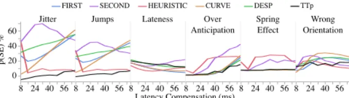
Jitter Jumps Lateness Over Anticipation Spring Effect Wrong Orientation p(SE ) % 60 40 20 0 8 24 40 56 8 24 40 56 8 24 40 56 8 24 40 56 8 24 40 56 8 24 40 56 Latency Compensation (ms)

FIRST SECOND HEURISTIC CURVE DESP TTp

Figure 3: Effects of Compensated Latency and Predictor on the proba-bility to notice each side-effect.

amount of compensated latency and the probability of indi-vidual negative side-effect.

Looking for effects of Predictor and Compensated Latency on the probability p(SE) to notice a side-effect, we ran a mixed-design analysis of variance for each side-effect, considering participant as random variable. Unsurprisingly (Fig. 3), we found significant effects of Predictor, Compensated Latency, and Predictor ⇥ Compensated Latency, all p < 0.001. We will not detail the later two further than Fig. 3.

What interests us here is how TTPfared against other predic-tors overall. Post-hoc Tukey tests showed that TTPcaused

significantly less Jitter (mean 1.6% vs. 11.9 to 56.9%) and Jumps (3.2% vs. 10.8 to 37%) than any other predictor that we tested. It was significantly better on Wrong Orienta-tion (16.1%) than all other predictors (18.7 to 23.8%) except

HEURISTIC(14.5%) from which it wasn’t significantly

differ-ent. It was significantly better on Spring Effect (8.3%) than

HEURISTIC and SECOND (resp. 22.3 and 16.3%), and not

significantly different from the others (8 to 8.4%). It was sig-nificantly better at Over-anticipation (6.8 %) thanSECOND, HEURISTIC, andCURVE (resp. 20.8, 19.4, 9.2%), and not

significantly different from the others: DESP(8%) andFIRST

(8.3%). Finally, for Lateness, TTP(15.5%) was significantly

better thanSECOND(17.3%), significantly worse thanFIRST,

HEURISTIC, andCURVE(9.3 to 10.2%), and not significantly

different from DESP.

TTPemerges as the most stable predictor (lowest Jitter and

Jumps) by a significant margin, i.e. 7 to 36 times lower than other predictors, and belongs to the ‘best’ groups for all side-effects except Lateness. Interestingly, the other ‘best’ pre-dictors often swap rankings depending the side-effect under consideration. For instance,HEURISTIC was comparatively

as good for Wrong Orientation but among the worst in Over-anticipation; DESPwas among the best in Over-anticipation

and among the worst in Jitter. In short, existing predictors trade some side-effects for others, while TTPdemonstrates

probabilities of side-effects equivalent or lower than the best predictors for most individual side-effects.

Overall score

Regarding Lateness, this metric is calculated as the mean of distances between the predicted location of the finger and the actual location of the finger (without latency) when the predicted location is behind the direction of the movement. Predicted points that are ahead are not considered in this calculation: predictors that consistently over-anticipate, e.g.

(10)

More importantly, Lateness is essentially why prediction oc-curs in the first place, and therefore the main cause for all the other side-effects. Yet at the same time, it is the side-effect with the lowest Disturbance scores in [20] (Table 1), in which participants reportedly suggested that [perceived] latency was normal, and better than bad prediction errors.

We calculated a general prediction score SPfor each predictor

P consisting in the sum of the expected probability p(SEP)of

each side effect SE for this predictor, weighted by the distur-bance score Mo(D)SE from Table 1 for that side-effect:

SP=

Â

SE

p(SEP)⇥ Mo(D)SE (6)

We used this score to compare the predictors overall in terms of expected overall disturbance:

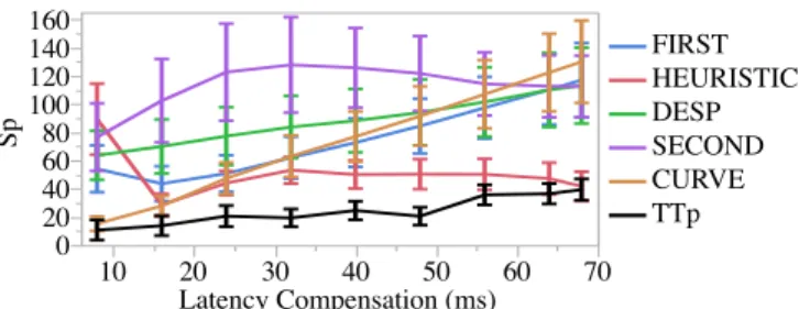
Sp 160 140 120 100 80 60 40 20 0 10 20 30 40 50 60 70 Latency Compensation (ms) FIRST HEURISTIC DESP SECOND CURVE TTp

Figure 4: Expected disturbance score per Predictor and Latency Com-pensation. Error bars are 95% confidence intervals.

Looking for effects of Predictor and Compensated Latency on the overall score SP, we ran a mixed-design analysis of

vari-ance, considering participant as random variable. Unsurpris-ingly (Fig. 4), we found significant effects of Predictor, Com-pensated Latency, and Predictor ⇥ ComCom-pensated Latency, all p < 0.001. We will not detail the later two further than Fig. 4. What interests us here is how TTP fared against other

pre-dictors overall. Post-hoc Tukey tests showed that TTP ob-tains scores (mean 24.6) significantly lower than any other Predictor overall. HEURISTIC comes second (50.6), signifi-cantly lower than any remaining Predictor. CURVE(75.7) is

significantly better than DESP (89.1), with FIRST

insignifi-cantly different from both. Finally,SECONDobtained scores

significantly worse than any other predictor (112.9).

To get a finer picture, we re-ran the above analyses for each amount of Compensated Latency. In each case, there was a significant effect of Predictor (p < .001), and Tukey post-hoc tests showed that TTPwas either significantly better or

non-significantly different from all other predictors in every case.

EXPERIMENT

In order to confirm the results of our benchmark, we ran a controlled experiment on an interactive tablet to gather and compare the opinions of real users on the aforementioned pre-dictors. The experiment involved performing different tasks and different amounts of compensated latency. Participants were asked to rate the acceptability of each condition (Pre-dictor ⇥ Task ⇥ Latency compensation). That yielded sig-nificantly more conditions than in [20] (through the Latency compensation factor), so we asked participants to report ex-isting side-effects rather than describe all issues themselves.

Participants

We recruited 9 participants: 2 left-handed, 2 female, aged 22 to 41 (µ 30.8, s 7.9). All were frequent computer users and used touch input more than one hour per day. Participants were not compensated.

Apparatus

Experiment software was implemented in C++ using Qt 5.9 on an iPad Pro 10.5” (Model A1701) running iOS 11.2. Us-ing Casiez et al.’s method [3], we determined an average 52.8 ms latency (SD 2.8). To get a latency comparable to Nancel et al., who used a Microsoft Surface Pro with an average la-tency of 72.6 ms [20], we added 20 ms of artificial lala-tency by buffering touch events. In this way we can compare more easily the results of this experiment to the results of the sim-ulations. The iPad Pro’s input frequency is 120 Hz, the same as reported in [20].

Conditions

Compensated Latency

We presented participants with five levels of compensated la-tency: 0, 16, 32, 48, and 64 ms. That is a coarser granularity than in the benchmark above, but allowed us to experiment on different levels of latency compensation while ensuring that the experiment remained in realistic durations.

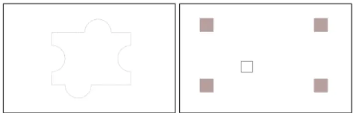
Tasks

We presented participants with three tasks:Drawing, similar to [20], in which participants were instructed to draw a shape that was displayed on the background of the tablet (Fig. 5-a) with their finger at different speeds, along with anything else they wanted; Dragging, also similar to [20], in which par-ticipants were instructed to drag a square object around with their finger and attempt to drop it within one of four square targets (Fig. 5-b), a task they could repeat as often as they wanted; andWriting, in which participants were instructed to write anything they wanted using their finger on the tablet. Specific minimization objectives such as “click the target as fast as you can” or “follow the shape as precisely as possi-ble” impose constraints on user movements, which in turn might favor—or hide—side-effects caused by slow vs. fast movements, straight vs. curved vs. angled trajectories, etc.; improving performance also does not necessarily mean less noticeable prediction side-effects. We therefore applied the same design as [20], i.e. looser instructions to encourage free exploration of the various conditions and favor larger ranges of “good” and “bad” predictor behaviors. Systematic assess-ment of performance with TTPis left for future work.

In all tasks the prediction was only used for immediate feed-back: last part of the stroke starting from the last detected in-put forWriting and Drawing, object location for Dragging. Traces, the dragged object’s location after release, and stored data if it were a real application, correspond to detected input.

Predictors

The predictors were the same as in the benchmark study:

FIRST,SECOND,HEURISTIC,CURVE,DESP, and TTP. The

(11)

Figure 5: Visual backgrounds of the tasks: (Left) in Drawing, a shape was displayed on the background, including straight and curves lines, and angles. (Right) in Dragging, four target squares were displayed at the corners of the display, slightly larger than the dragged object.

“Technique 2”, etc.). For TTPwe ran the optimization

de-scribed in subsection “Parameters Tuning” above (p. ), and calibrated the parameters of the 1e filter by hand, for each level of latency compensation. As a result of this tuning, fil-tering was deactivated for 16 ms, the Beta parameter [4] was set to zero in all remaining cases, and the cutoff frequency parameter was set to 45, 20, and 15 Hz respectively for 32, 48, and 64 ms of latency compensation.

Procedure

After being explained the goals and procedure of the experi-ment, participants were demonstrated each task on the tablet. A trial corresponds to one condition: Predictor, Task, Amount of compensated latency. In each trial, participants were in-structed to use the touch interface for as long as they wanted in order to form an opinion regarding (a) whether they no-ticed issues with the interface, (b) how disturbing those issues were, and whether that would in their opinion prevent its use in a real setting, and (c) which issue was observed among a subset of the side-effects list discussed in [20].

More precisely, after having spent some time in each condi-tion, participants were instructed to:

1. Rate the acceptability of the predictor in that condition on a scale with values “No noticeable issue” (1), “Noticeable issues, but fine” (2), “Some issues, still usable” (3), “Is-sues, barely usable” (4), and “Unbearable / unacceptable” (5)6_{; that scale mirrors the questionnaire used in [20],}

2. Tell whether they would not consider using this predictor in daily personal or professional use, and

3. If they would not, list the issues that justify that rejection from a list of side-effects composed of the six described in Table 1, and of two more reported by Nancel et al. as frequently used by their participants [20]:

The acceptability rating set (1. above) is in the form ”one neutral, four negatives”, as per the studied problem: our goal is to distinguish levels and types of “imperfectness” in the predictions. A perfect prediction feels normal, and can only be observed by comparison to imperfect ones, e.g. through lateness or unwanted interface behaviors.

Random: Could not understand the logic behind some as-pects or all of the prediction trajectory.

6_{Participants were presented the rating labels, not the corresponding}

numbers. For readability we only report numbers in what follows.

Multiple feedback: Seemed like more than one visible feed-back at the same time.

Participants could also describe issues that were not in the list, but no other side-effect was reported.

Design

The presentation of the predictors and tasks was counterbal-anced using two Latin Square designs, predictors first: all tasks were completed for a given predictor before switching to the next predictor. The ordering of the latency compensa-tion was constant and increasing, from 0 ms to 64 ms. In the end we obtained ratings and raw input and predicted data for 9 (participants) ⇥ 6 (predictors) ⇥ 3 (tasks) ⇥ 5 (la-tency) = 810 conditions. The study lasted 1 hour on average for each participant.

Results

We recorded a total of 10,270 strokes but removed the first 5th

duration percentile (< 12 ms) and last 5th_{percentile (> 4629}

ms) as Nancel et al. did [20], leaving a total of 9,242 strokes. In each Predictor⇥Task condition, participants spent on av-erage 1 min (SD 0.6) interacting with the touch surface (sum of stroke durations). Participants spent on average 2.9 min (1.1) interacting with each Predictor. A multi-way ANOVA reveals that Task had a significant effect on interaction dura-tion (F2,136 = 5, p = .0079), withWriting conditions (mean 0.8

min) taking significantly longer thanDrawing and Dragging (1 min).

Acceptability Ratings

Ratings in absolute value are represented in Fig. 6, aggregated for all participants and all tasks (the lower the better). As it could be expected, we observe strong discrepancies be-tween the ratings of each participant. For instance, two par-ticipants (P3, P7) never used ratings of 4 or above, one (P7) never used the 5th. Conversely, four participants (P5, P7-9) rated all amounts of compensated latency 3 or worse in at least one combination of Predictor ⇥ Task, including with the typical amounts of compensated latencies 0 and 16 ms. Despite that, visual inspection of the means and confidence intervals (CI) reveal a clear trend in favor of TTPoverall, and

for amounts of compensated latencies of 32 ms and above. We ran a multi-way ANOVA by treating acceptability rat-ings as continuous values between 1 and 5 (the lower the better), and modeling participant as a random variable using SAS JMP’s REML procedure. It confirmed that acceptability ratings were significantly affected by Predictor (F5,712 = 53.3, p < 0.0001), Task (F2,712 = 146.3, p < 0.0001), and Latency

(F4,712 = 243.3, p < 0.0001), as well as several interaction

effects: Predictor⇥Latency (F20,712 = 5.8, p < 0.0001) and

Predictor⇥Task (F10,712 = 5, p < 0.0001). TTP(mean 1.61)

was found significantly more acceptable than all other predic-tors (means 2.41). Unsurprisingly, acceptability ratings in-creased with the amount of compensated latency, every level being significantly different than the others. Conditions with TTPcompensating up to 48 ms of compensation (means 1.33

to 1.7) were found significantly more acceptable than all other predictors at 32 ms (2.48 to 3.15) and above. TTPwith up to

(12)

64 ms of compensation (2.22) was found significantly more acceptable than all other predictors at 48 ms (3.04 to 3.89) and above. A ccept abi lit y rat ing 0 ms 16 ms 32 ms 48 ms 64 ms

FIRST HEURISTIC DESP SECOND CURVE TTp

1 2 3 4 5

Figure 6: Left: Average ratings for each predictor. Right: Average rat-ings for each predictor and amount of compensated latency. Error bars are 95% confidence intervals.

Due to the variability in the range of each participant’ re-sponses, we also inspected the ordering of these ratings. For each (Participant ⇥ Task ⇥ Latency) combination, we ranked each predictor from best (1) to worst (5). We treated ties ‘op-timistically’: equal ratings were considered ex-æquo and to the lowest ranking; for instance, if in a given condition the predictors A, B, C, D, E, F had ratings of 1, 1, 2, 3, 4, 4, their corresponding rankings would be 1, 1, 3, 4, 5, 5.

With this method, TTP was ranked first (including ties)

92.6% of the time, second 6.7% of the time, third 0.7% of the time, and never further. By comparison, the other predic-tors were ranked first 29.6 to 45.2% of the time, second 33.3 to 45.2% of the time, third 12.6 to 28.9% of the time, and fourth 1.5 to 9.6% of the time.

If we break down these rankings per level of compensated latency, we find that TTP was only ever ranked third with

0 ms of compensation. For 16, 32, and 64 ms it was ranked first (incl. ties) respectively 85.2, 92.6, and 96.3% of the time, second the rest of the time. For 48 ms it was always ranked first. Except at 0 ms (where all predictors are equivalent), no other predictor come near this level of plebiscite.

To summarize, TTPobtained consistently better ratings than all other predictors, both in absolute value and in ranking. Participants’ average ratings ranged between 1 (“No notice-able issue”) and 2 (“Noticenotice-able issues, but fine”) in all condi-tions, including up to 48 and 64 (Fig. 6).

Rejection for Real Use

In each Predictor ⇥ Task ⇥ Latency condition, participants were asked whether they would not consider using this pre-dictor at this compensation setting in a similar task, for daily personal use and daily professional use (2 separate questions). It is not trivial to perform traditional statistical analyses on such a question as a single measure. We cannot simplify it as ‘the lowest level they started rejecting the predictor for that task’ because it happened that participants ticked the box for a given level of latency compensation and not for higher lev-els. The corresponding data is essentially a binary variable for every combination of Participant ⇥ Predictor ⇥ Task ⇥ Latency, which can only be studied as a whole by consider-ing histograms of responses. In what follows we limit our analysis to an inspection of number of responses.

Similarly to acceptability ratings, we observe a discrepancy between the participants’ tolerance to prediction side-effects. For instance, for personal use, three participants (P2, P5, P8) rejected predictors at least once for each amount of compen-sated latency, i.e. including when there was no latency com-pensation at all (0 ms), while five (P1, P3-4, P6-7) only re-jected conditions with 32 ms of compensation or higher; two (P3-4) only rejected conditions with 48 ms of compensation or higher. All participants but one (P8) were equally or more tolerant to perceived side-effects when considering personal use than when considering professional use. Counts of rejec-tions are represented in Fig. 7.

0 5 10 15 20 0 16 32 48 64 0 16 32 48 64

Unsuitable for personal use

Nb

of

respon

ses

Unsuitable for professional use

Amount of compensated latency (ms)

Figure 7: Number of times the participants responded that a particular condition (Predictor ⇥ Task ⇥ Latency) would not be suitable for real use, either personal or professional, by amount of predicted latency.

Upon simple visual inspection, we observe that participants’ rejection of the TTPpredictor tends to drop as the level of compensated latency increases, up until 32 and 48 ms for respectively personal and professional use. Rejection of all other predictors steadily increases starting from 0 or 16 ms.

Observed Side-effects

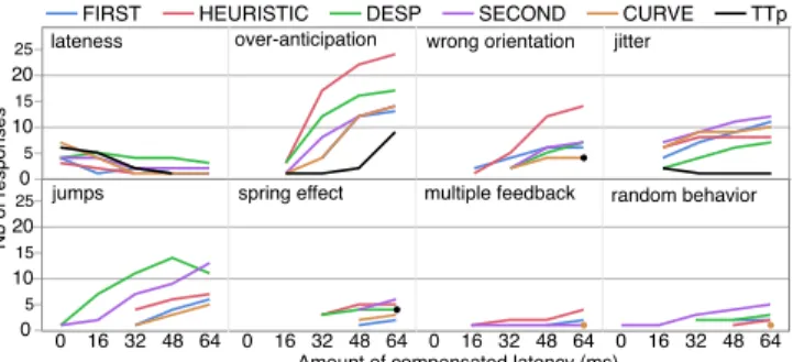
When a participant rejected a given condition, they were in-structed to indicate the causes for that rejection. These mea-sures have the same format as above: some participants for example reported “lateness” for low levels of compensation only and other issues starting from e.g. 32 ms. We therefore limit this analysis to an inspection of number of responses. Counts of mentions of each side-effect are shown in Fig. 8.

0 16 32 48 64 0 5 10 15 20

25 lateness over-anticipation wrong orientation jitter

jumps spring effect multiple feedback random behavior

0 16 32 48 64 0 16 32 48 64 0 16 32 48 64 0 5 10 15 20 25

Amount of compensated latency (ms)

Nb

of

respon

ses

Figure 8: Number of times the participants responded that a particular condition side-effect caused her rejection of a predictor for each level of compensated latency. Single points represent predictors for which a given side-effect was only reported for a unique level of compensation.

We can make several observations: (1) “Jumps” and “Ran-dom behavior” are reported at least once for all predictors except TTP; “Multiple feedback” is reported at least once for

(13)

“Wrong orientation” are reported for all predictors at least at 48 ms of compensation except for TTPfor which it is only

re-ported at 64 ms. (3) “Lateness” has been rere-ported for all pre-dictors, and at all levels of compensation except forHEURIS -TICat 48 ms and above, and for TTPat 64 ms; while among

the highest for 0 and 16 ms, reports of “Lateness” with TTP

quickly drop starting from 32 ms. (4) “Jitter” and “Over-anticipation” were reported at all levels above 0 ms for every predictor, but remain consistently lowest for TTP.

Breaking Down by Task

Inspecting the above results task by task reveals trends sim-ilar to [20]. “Lateness” was mostly reported withDragging (77.9% of reports), possibly because the finger was hiding most of the delay (inDrawing and Writing the prediction was connected to the last detected point by the stroke), and because participants are used to latency in direct touch. “Jit-ter” and “Jumps” were mostly reported withDragging (resp. 77.2 and 75.2%), again possibly because the finger was hid-ing most of the tremblhid-ing—in contrast, the dragged object was larger than the finger. “Over-anticipation” was reported at lower levels of compensation withWriting than with the two other tasks: all predictors butFIRSThad reports at 16 ms

in this task, while inDragging and Drawing the reports start at 32, 48, or 64 ms. This is possibly because writing gestures are curvier and, being heavily practiced, faster than drawing and dragging gestures, eliciting brisker responses from the predictors. Finally, “Over-anticipation” was only reported at 64 ms of compensation with TTPfor DRAGGINGand DRAW

-ING, while for all other predictors it was reported starting at

32 or 48 ms with these tasks.

Comparison with Benchmark Study

The findings from the benchmark and user studies were very similar: TTPwas found consistently less disturbing both in

theory (benchmark, see e.g. Fig. 4) and in practice (controlled study, Fig. 6-7). Issues of jitter, jumps, and spring effect were very seldom reported (Fig. 8), as predicted (Fig. 3). Reports of over-anticipation stayed low until 48 ms before rising sud-denly, in both cases. Finally, some side-effects went even better in practice than predicted: reports of lateness experi-enced a steady drop starting from 32 ms, and disappeared for 64 ms; and wrong orientation was only observed at 64 ms. Overall, the results of both studies speak in favor of using TTPat higher levels of latency compensation than the other

predictors we tested. Participants ‘rejected’ the use of TTP

for professional use less often at 32 and 48 ms of com-pensated latency than at any other amount, including 0 ms (Fig. 7). All side-effects but lateness, over-anticipation, and jitter were never reported for TTPat these levels of compen-sation, and the latter three were minimal compared to other predictors. This, we conclude, strongly supports our hypoth-esis that TTPcan be used to forecast direct touch input further

in the future than existing approaches.

DISCUSSION AND FUTURE WORK

We presented a new algorithm for next-point input prediction based on three components: (i) a state-of-the-art differentia-tor to quickly and accurately estimate the instantaneous time

derivatives of the input movement in real time, (ii) a speed-based smoothing mechanism to solve the lateness/jitter trade-off, and (iii) a two-step filtering of the resulting prediction to further decrease jitter without sacrificing angular responsive-ness. The effectiveness of the resulting predictor, as demon-strated in a benchmark and a user study, can result from any or all of these components. In effect, the speed-based smoothing and two-steps filtering could theoretically benefit any predic-tion algorithm. The study of the individual effects of each component is left for future work.

We will also investigate the efficiency of TTP when using

other common devices such as direct styli and indirect mice, and whether the calibration processes need to be adjusted in those setups.

Finally, predictors using more complex approaches such as Kalman filters and neuron networks could not be tested in this work for lack of accessible calibration procedures, but those approaches are very promising and we would like to compare them to our predictor in future work.

CONCLUSION

We presented a new prediction technique for direct touch sur-faces that is based on a state-of-the-art finite-time derivative estimator, a smoothing mechanism based on input speed, and a two-step post-filtering of the prediction. Using the dataset of touch input from Nancel et al. as benchmark we compared our technique to the ones of the state-of-the-art, using met-rics that model user-defined negative side-effects caused by input prediction errors. The results show that our prediction technique presents probabilities of side-effects equivalent or lower than the best predictors for most individual side-effects. This was confirmed in a user study in which participants were asked to rate the disturbance of existing predictors at different levels of latency compensation: our technique shows the best subjectives scores in terms of usability and acceptability. It remains usable up to 32 or 48 ms of latency compensation, i.e. two or three times longer than current techniques.

ACKNOWLEDGMENTS

This work was supported by ANR (TurboTouch, ANR-14-CE24-0009).

REFERENCES

1. 2014. Curve fitting based touch trajectory smoothing method and system.

https://www.google.ca/patents/CN103902086A?cl=enCN

Patent App. CN 201,210,585,264.

2. S. Aranovskiy, R. Ushirobira, D. Efimov, and G. Casiez. 2017. Frequency domain forecasting approach for latency reduction in direct human-computer interaction. In 2017 IEEE 56th Annual Conference on Decision and Control (CDC). 2623–2628. DOI:

http://dx.doi.org/10.1109/CDC.2017.8264040

3. G´ery Casiez, Thomas Pietrzak, Damien Marchal, S´ebastien Poulmane, Matthieu Falce, and Nicolas Roussel. 2017. Characterizing Latency in Touch and Button-Equipped Interactive Systems. In Proceedings of

(14)

the 30th Annual ACM Symposium on User Interface Software and Technology (UIST ’17). ACM, New York, NY, USA, 29–39. DOI:

http://dx.doi.org/10.1145/3126594.3126606

4. G´ery Casiez, Nicolas Roussel, and Daniel Vogel. 2012. 1e Filter: A Simple Speed-based Low-pass Filter for Noisy Input in Interactive Systems. In Proc. SIGCHI Conference on Human Factors in Computing Systems (CHI ’12). ACM, 2527–2530. DOI:

http://dx.doi.org/10.1145/2207676.2208639

5. Elie Cattan, Amélie Rochet-Capellan, Pascal Perrier, and François Bérard. 2015. Reducing Latency with a Continuous Prediction: Effects on Users’ Performance in Direct-Touch Target Acquisitions. In Proc. 2015 International Conference on Interactive Tabletops and Surfaces (ITS ’15). ACM, 205–214. DOI:

http://dx.doi.org/10.1145/2817721.2817736

6. Jonathan Deber, Ricardo Jota, Clifton Forlines, and Daniel Wigdor. 2015. How Much Faster is Fast Enough? User Perception of Latency & Latency Improvements in Direct and Indirect Touch. In Proceedings of the 33rd Annual ACM Conference on Human Factors in Computing Systems (CHI ’15). ACM, New York, NY, USA, 1827–1836. DOI:

http://dx.doi.org/10.1145/2702123.2702300

7. T. E. Duncan, P. Mandl, and B. Pasik-Duncan. 1996. Numerical differentiation and parameter estimation in higher-order linear stochastic systems. IEEE Trans. Automat. Control 41, 4 (Apr 1996), 522–532. DOI:

http://dx.doi.org/10.1109/9.489273

8. D. V. Efimov and L. Fridman. 2011. A Hybrid Robust Non-Homogeneous Finite-Time Differentiator. IEEE Trans. Automat. Control 56, 5 (May 2011), 1213–1219.

DOI:http://dx.doi.org/10.1109/TAC.2011.2108590

9. Michel Fliess, C´edric Join, and Hebertt Sira-Ramirez. 2008. Non-linear estimation is easy. Int. J. Modelling, Identification and Control 4, 1 (2008), 12–27. DOI:

http://dx.doi.org/10.1504/IJMIC.2008.020996

10. Niels Henze, Markus Funk, and Alireza Sahami Shirazi. 2016. Software-reduced Touchscreen Latency. In Proceedings of the 18th International Conference on Human-Computer Interaction with Mobile Devices and Services (MobileHCI ’16). ACM, New York, NY, USA, 434–441. DOI:http://dx.doi.org/10.1145/2935334.2935381

11. Niels Henze, Sven Mayer, Huy Viet Le, and Valentin Schwind. 2017. Improving Software-reduced Touchscreen Latency. In Proceedings of the 19th International Conference on Human-Computer Interaction with Mobile Devices and Services

(MobileHCI ’17). ACM, New York, NY, USA, Article 107, 8 pages. DOI:

http://dx.doi.org/10.1145/3098279.3122150

12. Ricardo Jota, Albert Ng, Paul Dietz, and Daniel Wigdor. 2013. How Fast is Fast Enough? A Study of the Effects of Latency in Direct-touch Pointing Tasks. In

Proceedings of the SIGCHI Conference on Human Factors in Computing Systems (CHI ’13). ACM, New York, NY, USA, 2291–2300. DOI:

http://dx.doi.org/10.1145/2470654.2481317

13. B. Kim and Y. Lim. 2014. Mobile terminal and touch coordinate predicting method thereof.

https://www.google.com/patents/WO2014129753A1?cl=en

WO Patent App. PCT/KR2014/000,661. 14. Joseph J. LaViola. 2003. Double Exponential

Smoothing: An Alternative to Kalman Filter-based Predictive Tracking. In Proc. Workshop on Virtual Environments 2003 (EGVE ’03). ACM, 199–206. DOI:

http://dx.doi.org/10.1145/769953.769976

15. Arie Levant. 1998. Robust exact differentiation via sliding mode technique. Automatica 34, 3 (1998), 379 – 384. DOI:http://dx.doi.org/10.1016/S0005-1098(97)00209-4

16. Jiandong Liang, Chris Shaw, and Mark Green. 1991. On Temporal-spatial Realism in the Virtual Reality

Environment. In Proc. 4th Annual ACM Symposium on User Interface Software and Technology (UIST ’91). ACM, 19–25. DOI:

http://dx.doi.org/10.1145/120782.120784

17. J.S. LINCOLN. 2013. Position lag reduction for computer drawing.

https://www.google.com/patents/US20130271487US Patent

App. 13/444,029.

18. F. Moussavi. 2014. Methods and apparatus for incremental prediction of input device motion.

https://www.google.ca/patents/US8766915US Patent

8,766,915.

19. Tomas M´enard, Emmanuel Moulay, and Wilfrid Perruquetti. 2017. Fixed-time observer with simple gains for uncertain systems. Automatica 81, Supplement C (2017), 438 – 446. DOI:http://dx.doi.org/https:

//doi.org/10.1016/j.automatica.2017.04.009

20. Mathieu Nancel, Daniel Vogel, Bruno De Araujo, Ricardo Jota, and G´ery Casiez. 2016. Next-Point Prediction Metrics for Perceived Spatial Errors. In Proceedings of the 29th Annual Symposium on User Interface Software and Technology (UIST ’16). ACM, New York, NY, USA, 271–285. DOI:

http://dx.doi.org/10.1145/2984511.2984590

21. Albert Ng, Michelle Annett, Paul Dietz, Anoop Gupta, and Walter F. Bischof. 2014. In the Blink of an Eye: Investigating Latency Perception During Stylus Interaction. In Proceedings of the 32Nd Annual ACM Conference on Human Factors in Computing Systems (CHI ’14). ACM, New York, NY, USA, 1103–1112.

(15)

22. Albert Ng, Julian Lepinski, Daniel Wigdor, Steven Sanders, and Paul Dietz. 2012. Designing for

Low-latency Direct-touch Input. In Proceedings of the 25th Annual ACM Symposium on User Interface Software and Technology (UIST ’12). ACM, New York, NY, USA, 453–464. DOI:

http://dx.doi.org/10.1145/2380116.2380174

23. Wilfrid Perruquetti, Thierry Floquet, and Emmanuel Moulay. 2008. Finite-time observers: application to secure communication. Automatic Control, IEEE Transactions on 53, 1 (2008), 356–360. DOI:

http://dx.doi.org/10.1109/TAC.2007.914264

24. R. Ushirobira, D. Efimov, G. Casiez, N. Roussel, and W. Perruquetti. 2016. A forecasting algorithm for latency compensation in indirect human-computer interactions. In 2016 European Control Conference (ECC).

1081–1086. DOI:

http://dx.doi.org/10.1109/ECC.2016.7810433

25. W.Q. Wang. 2013. Touch tracking device and method for a touch screen.

App. 13/367,371.

26. W. Wang, X. Liu, and G. ZHOU. 2013. Multi-touch tracking method.

https://www.google.com/patents/WO2013170521A1?cl=en

WO Patent App. PCT/CN2012/077,817.

27. Jiann-Rong Wu and Ming Ouhyoung. 2000. On latency compensation and its effects on head-motion trajectories in virtual environments. The Visual Computer 16, 2 (2000), 79–90. DOI:

http://dx.doi.org/10.1007/s003710050198

28. W. Zhao, D.A. Stevens, A. Uzelac, H. Benko, and J.L. Miller. 2012. Prediction-based touch contact tracking.

App. 13/152,991.

29. S.Q. Zhou. 2014. Electronic device and method for providing tactile stimulation.