Scheduling analysis of tasks constrained by TDMA: Application to software radio protocols

HAL Id: hal-01685444

https://hal.univ-brest.fr/hal-01685444

Submitted on 16 Jan 2018

HAL is a multi-disciplinary open access

archive for the deposit and dissemination of

sci-entific research documents, whether they are

pub-lished or not. The documents may come from

teaching and research institutions in France or

L’archive ouverte pluridisciplinaire HAL, est

destinée au dépôt et à la diffusion de documents

scientifiques de niveau recherche, publiés ou non,

émanant des établissements d’enseignement et de

recherche français ou étrangers, des laboratoires

Scheduling analysis of tasks constrained by TDMA:

Application to software radio protocols

Shuai Li, Frank Singhoff, Stéphane Rubini, Michel Bourdellès

To cite this version:

Shuai Li, Frank Singhoff, Stéphane Rubini, Michel Bourdellès. Scheduling analysis of tasks constrained

by TDMA: Application to software radio protocols. Journal of Systems Architecture, Elsevier, 2017,

76, pp.58-75. �10.1016/j.sysarc.2016.11.003�. �hal-01685444�

Scheduling Analysis of Tasks Constrained by

TDMA: Application to Software Radio Protocols

Author’s version

Shuai Li+*, Frank Singhoff*, St´ephane Rubini*,

Michel Bourdell`es+

*Lab-STICC UMR 6285, Universit´e de Bretagne

Occidentale, France, {last-name}@univ-brest.fr

+Thales Communications & Security, France,

{first-name}.{last-name}@thalesgroup.com

July 20, 2017

Abstract:

The work, presented in this article, aims at performing scheduling analy-sis of Time Division Multiple Access (TDMA) based communication systems. Products called software radio protocols, developed at Thales Communications & Security, are used as case-studies.

Such systems are real-time embedded systems. They are implemented by tasks that are statically allocated on multiple processors. A task may have an execution time, a deadline and a release time that depend on TDMA con-figuration. The tasks also have dependencies through precedence and shared resources. TDMA-based software radio protocols have architecture character-istics that are not handled by scheduling analysis methods of the literature. A consequence is that existing methods give either optimistic or pessimistic analysis results.

We propose a task model called Dependent General Multiframe (DGMF) to capture the specificities of such a system for scheduling analysis. The DGMF task model describes, in particular, the different jobs of a task, and task depen-dencies. To analyze DGMF tasks, we propose their transformation to real-time transactions and we also propose a new schedulability test for such transactions. The general analysis method is implemented in a tool that can be used by software engineers and architects. Experimental results show that our

proposi-tions give less pessimistic schedulability results, compared to fundamental meth-ods. The results are less pessimistic for both randomly generated systems and real case-studies from Thales.

These results are important for engineering work, in order to limit the over-dimensioning of resources. Through tooling, we also automated the analysis. These are advantages for engineers in the more and more competitive market of software radios.

Keywords: Real-time Embedded System, Scheduling Analysis, Task Depen-dency, Software Radio Protocol, TDMA, General Multiframe, Transaction

1

Introduction

In this article, we propose a scheduling analysis method for communication systems that use the Time Division Multiple Access (TDMA) channel access method. Our method is applied to real industrial systems, developed at Thales Communications & Security, called software radio protocols.

1.1

Context

Radios are communication systems. For communication to be established, some radio protocols need to be defined and implemented. Traditionally radios are implemented as dedicated hardware components. Trends in the last two decades have seen the emergence of software radios [1], where more and more components are implemented as software. This is the case for the radio protocol, which is then called a software radio protocol.

Software radio protocols are typical real-time systems. In such systems, activities are implemented by software tasks that are time-constrained. The tasks may also have precedence dependencies and use shared resources. In this article, we consider tasks that are scheduled by a partitioned Fixed Priority (FP) preemptive scheduling policy.

The particularity of a software radio protocol real-time system is that it may be impacted by TDMA, a common method to access the shared communication medium between several radio stations. In TDMA [2], time is divided into several time slots and at each time slot, a radio either transmits its data, or receives some data. This method impacts the software of the system, because the tasks have an execution time, deadline, and release time that depend on the time slots. TDMA is also one reason, among others, that there are hard deadlines in such systems. We must thus analyze the scheduling of these systems.

Scheduling analysis [3, 4] is the method used to verify that tasks will meet their deadline, when they are scheduled on processors. Scheduling analysis can potentially be complex, due to the dependencies between the tasks for example. Some methods, part of scheduling analysis, are schedulability tests [5]. Such tests assesses if all jobs, of all tasks, will meet their deadlines during execu-tion, when the tasks are scheduled on processors by a specific scheduling policy. Schedulability tests may compute the Worst Case Response Time (WCRT) of

tasks. The WCRT of a task is compared to its deadline to assess its schedula-bility.

Schedulability tests are associated with task models that abstract the archi-tecture of a real-time system for the analysis. There are several task models in the literature that consider more or less dependencies between tasks, and characteristics of the execution platform that hosts the tasks.

1.2

Overview of Contributions

As we will see, current task models and schedulability tests are not applicable to a software radio protocol that uses TDMA to access the shared communication medium. For example some task models may consider the impact of TDMA on tasks, but they do not consider task dependencies. Therefore, in this article we propose a scheduling analysis method adapted for the characteristics of real software radio systems developed at Thales. Our analysis method is based on several of our contributions. The next paragraphs describe our contributions and give an overview of our approach.

Extension of the General Multiframe Task Model This article proposes the Dependent General Multiframe (DGMF) task model, an extension of the General Multiframe (GMF) task model [6]. A GMF task is a vector of frames that represent the jobs of the task. The jobs may not have the same parameters, such as deadline and execution time. The DGMF task model extends GMF with precedence dependencies and shared resources. Contrary to GMF, the DGMF task model can also be applicable to a multiprocessor system with partitioned scheduling.

DGMF to Transaction The analysis method for DGMF consists in exploit-ing another kind of model called transactions [7]. A transaction is a group of tasks related by precedence dependency. This article proposes an algorithm to transform DGMF tasks to transactions. The transformation solves the issue of the semantic gap between the two models.

Extension of Schedulability Test for Transactions The transactions that are the results of the transformation have what we call non-immediate tasks, i.e. tasks which are not necessarily released immediately by their predecessor. Thus this article proposes the WCDSOP+NIM test, which is an extension of the WCDOPS+ test in [8]. Our test is used to assess schedulability of transactions with non-immediate tasks. Thanks to WCDSOP+NIM, we are able to perform scheduling analysis on transactions produced from DGMF models, and thus to perform scheduling analysis on DGMF models themselves.

Available Tool The GMF, DGMF, transaction models, and their analy-sis methods, are all implemented in Cheddar [9]. Cheddar is an open-source

TDMA Frame

S B B T T T T

Figure 1: TDMA Frame

scheduling analysis tool, available for both the research and industrial commu-nities.

1.3

Article Organization

The rest of this article is divided into five sections that are organized as follows. In Section 2, the TDMA-based software radio protocol system is presented. This section defines the assumptions of our work. In Section 3, we discuss the applicability of task models related to our work. In Section 4, the DGMF task model, and its analysis method, and experiments (both simulation results and case-study results) are exposed. Section 5 is on our WCDOPS+NIM schedula-bility test. Again, experiments on our test are shown in the same section, with both simulation results and case-study results. Finally, we conclude in Section 6 by discussing some future works.

2

Software Radio Protocol

In the following sections, we first present the concept of a radio protocol and the impact of TDMA on the protocol. Afterwards the software and execution platform of our system is presented, and we relate the architecture of the system to two typical architecture designs. Finally, we summarize the requirements to consider for our scheduling analysis work.

2.1

Radio Protocols Based On Time-Division

Multiplex-ing

A radio protocol is a set of rules to respect so communication can be established between different users on a same network. A radio protocol defines the syntax and semantics of the messages exchanged between users, but also how communi-cation is synchronized between all users. Several protocols can cooperate within a same radio to form the protocol stack [10].

The functionalities of a radio protocol may be impacted by the method used by the radio to access the communication medium. TDMA [2] is a channel access method, based on time-division multiplexing. It allows several radio stations to transmit over a same communication medium. In TDMA, time is divided into several time slots, called TDMA slots. At each slot, each radio station in the network either transmits or receives. The sequence of slots is represented as a TDMA frame. Figure 1 shows a typical frame.

Slots may be of different types. For example in Figure 1, the TDMA frame has three types of slot: Service (S ) for synchronization between stations; Bea-con (B ) for observation/signaling the network; Traffic (T ) for payload trans-mission/reception. Slots of different types do not necessarily have the same characteristics. One of the characteristics of a slot is its duration. Therefore slots of different types do not necessarily have the same duration. For example in Figure 1, a B slot duration is shorter than a S and T slot duration. The TDMA frame duration is the sum of durations of its slots. Slots can either be in transmission (Tx ), reception (Rx ), or Idle mode. In a Tx slot, a radio station can thus transmit data. When a radio station can transmit in a slot, we say that the slot is allocated to the station. A TDMA configuration defines the combination of slots, of different types, in a TDMA frame. A TDMA frame is repeated after it finishes. An instance of a frame is a cycle.

When TDMA is used to access the communication medium, it impacts the functionalities of the radio protocol and it introduces time constraints. For example the operation to fetch data packets to be transmitted in a Tx slot is time-constrained. The TDMA method is a particular case of the timed-token protocol for real-time communications [11]. Indeed the same approach of dividing time into time slots, and allocating slots to entities, is used in both methods. Since these methods introduce time constraints, tasks that implement the system may also have time constraints.

The next section exposes the software and execution platform architecture of one possible implementation of a radio protocol.

2.2

Software and Execution Platform Architecture

The previous section showed how a radio protocol is designed. This section presents one possible implementation by Thales, called a software radio pro-tocol [1]. The implementation is described through its software and execution platform architecture.

Traditionally functionalities of a radio protocol are implemented as dedi-cated hardware (e.g. ASIC, FPGA). There is no concurrency to access these computing resources. Scheduling analysis is thus not necessary. In the case of systems developed at Thales, the majority of the functionalities of the protocol is implemented as software running on a General Purpose Processor (GPP). The software entities are implemented by some entities in the execution platform: OS and hardware. Figure 2 shows an example of these entities.

Figure 2, shows several protocols (called RLC and MAC) implemented by tasks allocated on processors. The system is a partitioned multiprocessor sys-tem: tasks are allocated on a processor, and they do not migrate. On a proces-sor, tasks are scheduled by a preemptive FP scheduling policy. The priorities of tasks are assigned arbitrarily according to domain expertise.

They may have precedence dependency (e.g. communication through semaphores signaling). They may also use shared resources. Shared resources are assumed local [12], i.e. two tasks can use a shared resource only if they are allocated on the same processor. Shared resources are protected by a resource access

proto-Periodic Sporadic

TDMA Tick Release

Event Task Shared Resource Precedence Dependency Allocation

Figure 2: Architecture for Scheduling Analysis: Red CPU is a GPP handling ciphered data, Black CPU is a GPP handling deciphered data, DSP means Digital Signal Processor

col that prevents unbounded priority inversion for uniprocessor. Examples of such resource access protocols are PIP and PCP [13]. Their implementation can typically be found in execution platforms with the VxWorks OS. This OS is present in some products developed by Thales.

Some tasks may be released sporadically. For example some tasks are typi-cally released upon arrival of IP packets, which depends on the user application. Other tasks are released at pre-defined times. This is the case for tasks of a Medium Access Control (MAC) protocol [10]. In this article, activities of MAC are divided in time due to the usage of TDMA to access the communication medium. The releases of a task can follow a periodic pattern or a pattern de-fined by TDMA slots. Events called TDMA ticks indicate the start of a slot and thus the release of some tasks. Tasks that are released at the start of a slot may also have execution times and deadlines that are constrained by the slot.

The software architecture of the system is conform to some architectures found in the literature. Indeed, two software architectures for RTES have been studied extensively: event-triggered [14] and time-triggered [15]. A software radio protocol is both a time-triggered and an event-triggered system. Indeed, some tasks are released by TDMA ticks indicating the start of a slot. Thus certain tasks are released at pre-defined times, which is conform to the time-triggered architecture. On the other hand, there are also tasks released by sporadic events, for example upon arrival of IP packets. Due to precedence dependency, a task can also be released by an event produced by a predecessor task.

2.3

Requirements for Scheduling Analysis

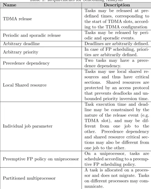
From the description of its architecture in Section 2.2, characteristics of a soft-ware radio protocol, useful for scheduling analysis, are summarized in Table 1. In this article, it is expected that the proposed scheduling analysis method covers all of the characteristics in Table 1.

In the next section we study the applicability of scheduling analysis methods of the literature, when considering the requirements exposed in this section.

3

Applicability of Related Works

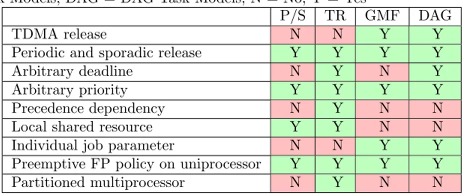
In this section, we discuss problems encountered when applying existing task models of the literature, to analyze the scheduling of a software radio protocol. A task model is said applicable to a characteristic of the system, if it is possible to model the characteristic, and if there exists a schedulability test for the task model that considers the characteristic. Table 2 shows the applicability of some task models to each characteristic. These task models come from the literature and they are the fundamental periodic task model [3], the transaction model [7] that expresses precedence dependent tasks, the multiframe task models [6] that express jobs of a task as a vector, and the DAG task models [5] that express jobs of a task as a graph.

The applicability of the task models is discussed in the following paragraphs. Either the non-applicability of some task models on a characteristic is justified, or the applicability of all task models on a characteristic is shown.

TDMA release Seminal schedulability tests in [3, 16] for the fundamental periodic and sporadic task models assume a synchronous system, where tasks are all released at a unique critical instant. Tasks constrained by TDMA are not synchronous since they may be released at different pre-defined times.

The transaction model, that generalizes the fundamental periodic and spo-radic task models, focuses on asynchronous releases of tasks. Tasks are said asynchronous if there is at least one first job of a task that is not released at the same time as the other first jobs of other tasks. In [7], Tindell analyzes asyn-chronous tasks with the transaction model. He takes the example of a network with a bus and messages scheduled by TDMA. His goal was not to analyze the effect that TDMA has on the scheduling of tasks within a single system (e.g. job execution time and release time constrained by the TDMA slot), but end-to-end response times of message transiting in the whole network. For example Tindell computes the response time from the sending of a message by a task, to the transition of the message on the bus, to the reception by another task.

Some other schedulability tests for transactions in [17, 8] also consider that there are some periodic tasks, and some tasks released immediately by their predecessor, instead of pre-defined times. These results cannot be applied on the targeted systems of this article.

Table 1: Requirements for Scheduling Analysis

Name Description

TDMA release

Tasks may be released at pre-defined times, corresponding to the start of TDMA slots, accord-ing to the TDMA configuration Periodic and sporadic release Tasks may be released by

peri-odic and sporadic events. Arbitrary deadline Deadlines are arbitrarily defined. Arbitrary priority In case of FP scheduling,

priori-ties are arbitrarily defined. Precedence dependency Two tasks may have a

prece-dence dependency.

Local Shared resource

Tasks may use local shared re-sources and thus have critical sections. Shared resources are protected by an access protocol that prevents deadlocks and un-bounded priority inversion time.

Individual job parameter

Task execution time and dead-line may be constrained by the nature of the release event (e.g. TDMA slot), and may be dif-ferent from one job to the other. Precedence dependency and shared resource critical sec-tions may also be different from one job to the other.

Preemptive FP policy on uniprocessor

On a uniprocessor, tasks are scheduled according to a preemp-tive FP scheduling policy.

Partitioned multiprocessor

A task is allocated on a proces-sor and does not migrate. Tasks on different processors may com-municate.

Table 2: Applicability of Task Models to Software Radio Protocol: Abbrevi-ations are P/S = Periodic/Sporadic, TR = Transactions, GMF = Multiframe Task Models, DAG = DAG Task Models; N = No, Y = Yes

P/S TR GMF DAG

TDMA release N N Y Y

Periodic and sporadic release Y Y Y Y

Arbitrary deadline N Y N Y

Arbitrary priority Y Y Y Y

Precedence dependency N Y N N

Local shared resource Y Y N N

Individual job parameter N N Y Y

Preemptive FP policy on uniprocessor Y Y Y Y

Partitioned multiprocessor N Y N N

Finally some works have been done on systems that are both event-triggered and time-triggered, like a software radio protocol. In [18], the authors work on an automotive system respecting the design of both architectures. Their work does not focus on task scheduling, but network scheduling. Indeed, their objective is to optimize the TDMA slot duration, when a bus is accessed by several processors through the TDMA channel access method.

Periodic and sporadic release All task models support tasks released by a periodic or a sporadic event [3, 7, 6, 19].

Arbitrary deadline Some of the schedulability tests for the periodic and sporadic task models assume Di≤ Ti [3, 16]. Thus the deadline is constrained.

Schedulability tests [6, 20] for GMF assume that the l-MAD property or the Frame Separation property hold. The l-MAD property constrains the deadline of a frame to be less than, or equal to, the deadline of the next frame. The Frame Separation property constrains the deadline of a frame to be less than the release of the next frame. These properties thus constrain the deadline of frames and thus tasks.

Arbitrary priority There exists at least one schedulability test for each task model that supports this characteristic [16, 21, 20, 5].

Precedence dependency Analysis of the periodic and sporadic task models did not fully handle precedence dependencies, until they were generalized by the transaction model [21].

Some works [22, 23, 7, 24] propose a method to schedule precedence de-pendent periodic or sporadic tasks. These methods either constrain the fixed priorities of tasks, or their deadlines, or they are proposed for a Earliest-Deadline First (EDF) policy with dynamic priorities instead of fixed one. Therefore they

are not applicable due to the arbitrary priorities, arbitrary deadlines, and FP scheduling policy of a software radio protocol.

Other works [25] also focus on periodic tasks with precedence dependencies that are not specified for every job, but every 2, 3, ..., n jobs. These works are not applicable to a software radio protocol, because precedence dependencies, among task jobs, do not follow this kind of pattern.

The multiframe task models assume independent tasks [6]. The DAG task models support precedence dependencies between jobs of a task. They do not explicitly handle precedence dependencies between the tasks themselves. For example the authors in [26] assume independent DAG tasks.

Local shared resource Like precedence dependencies, shared resources are not supported by the classical multiframe task models and DAG task models, since they assume independent tasks [6, 26]. In [27] the authors propose an optimal shared resource access protocol for GMF tasks but the protocol is not implemented in the OS of Thales products.

Individual job parameter The modeling of jobs with different parameters is only supported by the multiframe and DAG task models [6, 5, 26], among those present in Table 2.

Preemptive FP policy on uniprocessor All task models have schedulabil-ity tests for the preemptive FP scheduling policy [3, 7, 6, 26].

Partitioned multiprocessor The periodic, sporadic task models, and the multiframe task models have schedulability tests for uniprocessor systems [3, 6]. The DAG task models has tests for uniprocessor systems [5], or global multiprocessor systems [26], i.e. where tasks may migrate to other processors. Again, these task models are not applicable to our system.

In conclusion, the results of Table 2 show that none of the task models sup-port all characteristics of the software radio protocol to analyze. The following two sections expose our contributions to solve this problem: the DGMF task model, its transformation to a transaction model, and our extended schedula-bility test for transactions.

4

Dependent General Multiframe

To analyze the schedulability of a TDMA-based software radio protocol, this article proposes the Dependent General Multiframe (DGMF) task model. The following sections first define this task model. Then its analysis method is proposed. Finally some experimental results and evaluation are exposed.

4.1

DGMF, an Extension of GMF

Jobs with individual parameters is frequent in the multimedia domain. For example a video decoder task of a multimedia system has a sequence of images to decode. The parameters of a job of the task are constrained by the type of the image to decode. The described task behavior also occurs in software radio protocols. Indeed a job of a task, released by TDMA slots, may also have parameters constrained by the slot. The job parameters are thus constrained by the sequence of slots of the TDMA frame.

A task model motivated by the described behavior is the GMF task model. As a reminder, a GMF task is an ordered vector of frames representing its jobs. Each frame can have a different execution time, deadline, and minimum separation time from the frame’s release to the next frame’s release. Among task models that propose to model individual job parameters, GMF is sufficient for the modeling of a sequence of task jobs, constrained by a sequence of TDMA slots. On the other hand, GMF is limited to uniprocessor systems, without task dependencies, and with constrained deadlines. The GMF task model is thus extended to propose a task model called DGMF.

The DGMF task model extends the GMF model with task dependencies. It is also applicable to partitioned multiprocessor systems. The following sections first define the DGMF task model and its properties. Then an example is shown. Finally the applicability of GMF analysis method on DGMF is discussed. 4.1.1 DGMF Definitions and Properties

A DGMF task Giis a vector composed of Niframes F j

i, with 1 ≤ j ≤ Ni. Each

frame is a job of the same task Gi. Frames have some parameters inherited

from GMF:

• E_ij is the Worst Case Execution Time (WCET) of F_ij. • D_ij is the relative deadline of F_ij.

• P_ij is min-separation of F_ij, defined as the minimum time separating the release of F_ij and the release of F_ij+1.

A DGMF task also has a GMF period [6] inherited from the original task model. For DGMF task Gi with Ni frames, the GMF period Pi of Gi is:

Pi= Ni

X

j=1

P_ij (1)

Frames also have some parameters and notations specific to the DGMF task model:

• [U ]j_i is a set of (R, S, B) tuples denoting shared resource critical sections. F_ij asks for access to resource R after it has run S time units of its exe-cution time, and then locks the resource during the next S time units of its execution time.

• [Fq p]

j

iis a set of predecessor frames, i.e. frames from any other DGMF tasks

that must complete execution before F_ij can be released. A predecessor frame is denoted by Fq

p. Frame Fpq can only be in [Fpq] j

i if Giand Gp have

the same GMF period. When a frame Fy

x precedes F j i, the precedence dependency is denoted Fy x → F j i. We have ∀Fpq ∈ [Fpq] j i, Fpq → F j i. Fpq

are not the only frames that precede F_ij. For example, any frame that precedes a Fq p ∈ [Fpq] j i, also precedes F j i. For j > 1, we have F j−1 i → F j i.

• proc(F_ij) is the processor on which F_ij is allocated on. Critical section (R, S, B) can be in [U ]j_i and [U ]y x, with F j i 6= Fxy, only if proc(F j i) = proc(Fy x).

• prio(F_ij) is the fixed priority of F_ij (for FP scheduling). • rj_i is the first release time of F_ij. For the first frame F1

i, parameter r1i is

arbitrary. For the next frames, we have rj_i = r1

i + j−1 P h=1 Ph i.

Frames are released cyclically [6]. Furthermore, the first frame to be released by a DGMF task Gi is always the first frame in its vector, denoted by Fi1.

Parameter ri denotes the release time of Gi and we have ri= r1i.

A DGMF tasks set may have several properties. Let use define the Unique Predecessor property and the Cycle Separation property.

Property 1 (Unique Predecessor). Let F_ij be a frame of a task Gi, in a DGMF

tasks set. Let [Fq p]

j

i be the set of predecessor frames of F j i. F

j−1

i is the previous

frame of F_ij in the vector of Gi, with j > 1. The set of predecessor frames of

F_ij is the set [Fpq] j i and F

j−1

i (with j > 1).

A DGMF tasks set is said to respect the Unique Predecessor property if, for all frames F_ij, there is at most one frame Fy

x, in a reduced set of predecessors

of F_ij, with a global deadline (i.e. ry

x+ Dyx) greater than or equal to the release

time of F_ij. The reduced set of predecessors, of F_ij, are predecessors that do not precede another predecessor of F_ij.

To formally define the Unique Predecessor property, the set of predecessor frames of F_ij is denoted by pred(F_ij) such that:

pred(F_ij) = ( [Fq p] j i∪ {F j−1 i } with j > 1 [Fpq] j i otherwise. (2) Formally the Unique Predecessor property is then defined as follows:

∃≤1Fxy∈ pred(F j i) 0_{, r}y x+ d y x≥ max( max Fh l∈pred(F j i) (r_lh+ E_lh), rj_i) (3) where ∃≤1 means ”there exists at most one”, and the set pred(Fij)

0 _{is defined}

as:

pred(F_ij)0= pred(F_ij) \ {F_xy ∈ pred(F_ij) | ∃F_kl ∈ pred(F_ij), F_xy→ Fl

Table 3: DGMF Task Set E_ij Dj_i P_ij [U ]j_i [Fq p] j i prio(F j i) proc(F j i) G1; r1= 0 F₁1 1 4 1 F₂1 1 cpu1 F2 1 1 3 1 1 cpu2 F3 1 1 2 6 1 cpu1 F4 1 1 4 4 F22 1 cpu1 F5 1 4 8 8 (R, 1, 3) F23 1 cpu1 G2; r2= 0 F1 2 1 4 8 2 cpu1 F2 2 1 4 4 2 cpu1 F3 2 1 4 4 2 cpu1 F24 2 4 4 (R, 0, 1) 2 cpu1 G3; r3= 4 F31 1 2 2 F41 1 cpu1 F2 3 1 2 18 F42 1 cpu1 G4; r4= 4 F1 4 1 2 2 2 cpu1 F₄2 1 2 18 2 cpu1

Property 2 (Cycle Separation). A DGMF task Gi is said to respect the Cycle

Separation property if:

DNi

i ≤ ri+ Pi (5)

The Unique Predecessor and Cycle Separation properties simplify the anal-ysis method of DGMF so both properties are assumed for a DGMF tasks set. Experiments, presented later in this article, will show that they have no impact on the ability to model a real software radio protocol, developed at Thales, with DGMF.

To illustrate the task model defined in this section, the next section shows an example with some DGMF tasks, the parameters of their frames, and a possible schedule of the tasks set.

4.1.2 DGMF Example

Consider the DGMF tasks set in Table 3, modeling tasks constrained by a TDMA frame. Frames of G1 and G3 have a priority of 1. Frames of G2 and

G4 have a priority of 2. All frames are allocated on cpu1 except F12, which is

allocated on cpu2. Frames F5

1 and F24use a shared resource R.

Figure 3 shows an example of a schedule produced by the tasks set, over 20 time units. In the figure, the TDMA frame has 1 S slot, 2 B slots, and 3 T slots. Task G2 is released at S and T slots. G2 releases G1 upon completion. G4 is

released at B slots. G4 releases G3 upon completion. Release time parameter

example task G4 is released at time 4, which is the start time of the first B

slot. Notice that precedence dependencies are respected and F₄2 is blocked by F15 during 1 time unit, due to a shared resource.

4.1.3 Applicability of GMF Analysis Methods on DGMF

Schedulability tests exist for GMF tasks. In this section a test is reminded and its applicability to DGMF is discussed.

In [20] a response time based schedulability test for GMF tasks is proposed. This test assumes that tasks are independent and run on a uniprocessor system with a FP preemptive scheduling policy. Furthermore the authors also assume that the Frame Separation property holds: the relative deadline of a frame is less than or equal to its min-separation. Obviously this test cannot be applied to DGMF tasks for the following reasons:

• DGMF tasks have task dependencies

• DGMF frames may be allocated on different processors.

The next section proposes a scheduling analysis method for DGMF by ex-ploiting the transaction model.

4.2

DGMF Scheduling Analysis Using Transactions

In the previous section it was shown that GMF analysis methods cannot be applied to DGMF tasks because of task dependencies and the partitioned mul-tiprocessor nature of the system. Two choices are then available to solve this issue:

• Extend GMF schedulability tests

• Transform to another model where schedulability tests exist

The second approach is chosen in this article: DGMF tasks scheduling anal-ysis will be performed by transforming them to transactions. The transaction model is chosen for the following reasons:

• Task dependencies (precedence and shared resource) can be expressed. • Partitioned multiprocessor systems are considered.

• A independent GMF to transaction transformation is proposed in [28] for uniprocessor systems.

The transformation faces the issue of the difference in semantic between the two models. Indeed, transactions represent tasks related by collectively performed functionalities and timing attributes [7], not individual jobs of a task. The multiframe task models, on the other hand, express individual job parameters.

0 5 10 15 20 G 1 F 1 1 0 5 10 15 20 G 2 F 2 1 0 5 10 15 20 G 3 F 3 1 0 5 10 15 20 G 4 F 4 1 F 2 2 F 2 3 F 2 4 F 1 4 F 1 5 S B B T T T TDMA Frame F 3 2 F 4 2 0 5 10 15 20 F 1 2 F 1 3

Figure 3: Example of Schedule of DGMF Tasks: Up arrows are frame releases; Down arrows are frame relative deadlines; Dashed arrows are precedence de-pendencies; Curved arrows are shared resource critical sections where R is used; Crossed frame executes on a different processor

In the next sections, the transaction model is first reminded. Then the transformation algorithm in [28] is extended for DGMF tasks. Afterwards the DGMF tasks set in Section 4.1.2 is transformed to a transactions set. Finally schedulability tests for transactions are discussed to choose one suitable for transactions resulting from DGMF transformation.

4.2.1 Transaction Definitions

According to [29], ”a transaction is a group of related tasks (related either through some collectively performed function, or through some shared timing attributes whereby it is convenient to collect these tasks into a single entity)”. In [21], transactions are used to model groups of tasks related by precedence dependency. Let us see some definitions and notations for the transaction model, taken from [29, 7, 21, 17, 8].

A transaction is denoted by Γiand its tasks are denoted by τij. A transaction

is released by a periodic event that occurs every Ti. A particular instance of a

transaction is called a job. A job of a task in a transaction corresponds to a job of the transaction. If the event that releases the pth_{job of Γ}

ioccurs at t0, then

the pth_{jobs of its tasks are released after or at t}

0. The release time of the first

job of Γi is denoted by ri. A task τij has the following parameters:

• Cij is the WCET.

• Cb

ij is the Best Case Execution Time (BCET).

• Oij is the offset, a minimum time that must elapse after the release of the

job of Γi before τij is released [21]. Otherwise said τij is released at least

Oij units of time after t0. Value rij= ri+ Oij is the absolute release time

of the first job of τij.

• dij is the relative deadline. Value Oij+ dij is the global deadline [17] of

τij. Value ri+ Oij+ dij is the absolute deadline of the first job of τij.

• Jij is the maximum jitter, i.e. τij is released in [t0+ Oij; t0+ Oij+ Jij].

• Bijis the Worst Case Blocking Time (WCBT) [13] due to shared resources.

• prio(τij) is the fixed priority.

• proc(τij) is the processor on which τij is allocated on.

• Rw

ij is the global WCRT, which is the WCRT relative to the release of the

transaction [21]. A global response time is the response time of a task plus its offset. As a reminder, a response time of a task is relative to its release, in this case its offset.

• Rb

ij is the global Best Case Response Time (BCRT), which is the BCRT

Tasks may use shared resources in critical sections. A critical section is denoted by (τ, R, S, B) where τ is the task using the resource R. Task τ asks for R at S of its execution time, and locks it during the next B units of time of its execution time.

Tasks in a transaction are related by precedence dependencies [17]. A prece-dence dependency between two tasks is denoted by τip≺ τij. As a reminder, the

precedence dependency means that a job p of τip must complete before a job p

of τij can be released. τip (resp. τij) is called the predecessor (resp. successor)

of τij (resp. τip). According to the precedence dependencies that may exist

be-tween tasks, transactions are of different type. This article handles tree-shaped transactions.

Definition 1 (Tree-Shaped Transaction [8]). A tree-shaped transaction Γi has

a root task, denoted by τi1, which leads to the releases of all other tasks, upon

completion. A task τij, of a tree-shaped transaction, is said to have at most one

immediate predecessor (denoted by pred(τij)) that releases it upon completion.

A task τij may have several immediate successors (denoted by succ(τij)) that it

releases upon completion. The root task τi1 has no predecessor.

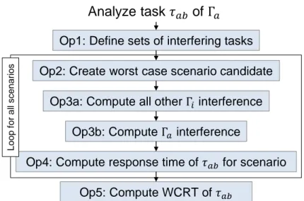
4.2.2 DGMF To Transaction

The DGMF to transaction transformation aims at expressing parameters and dependencies in the DGMF task model as ones in the transaction model. The transformation has three major steps:

• Step 1: Transform independent DGMF to transaction, i.e. consider DGMF tasks as independent and transform them to transactions. • Step 2: Express shared resource critical sections, i.e. model critical

sec-tions in the resulting transaction set and compute WCBTs.

• Step 3: Express precedence dependencies, i.e. model precedence depen-dencies in the transaction model.

In the following sections, each step is explained in detail.

Independent DGMF to Transaction Step 1 consists in transforming each DGMF task to a transaction by considering DGMF tasks as independent. Al-gorithm 4.2.2.1 shows the original alAl-gorithm proposed in [28] that is extended for DGMF tasks.

The idea behind the algorithm is to transform frames F_ij of a DGMF task Gi into tasks τij of a transaction Γi. Parameters in the transaction model,

like WCET (Cij), relative deadline (dij) and priority (prio(τij)), are computed

from parameters E_ij, Dj_i and prio(F_ij) from the DGMF model. To transform the min-separation of a frame in the DGMF model, offsets (Oij) are used in

the transaction model. The offset of a task τij is computed by summing the

Ph

i of frames Fih preceding F j

transformation, the release time ri of a DGMF task Gi is transformed into the

release time ri of a transaction Γi.

Algorithm 4.2.2.1 Independent DGMF to Transaction

1: for each DGMF task Gido

2: Create transaction Γi 3: 4: Ti← Ni P j=1 P_ij 5: Γi.ri← Gi.ri 6: 7: for each F_ijin Gido 8: Create task τij in Γi 9: 10: Cij← Eij 11: dij← Dji 12: Jij← 0 13: Bij← 0 14: prio(τij) ← prio(Fij) 15: proc(τij) ← proc(Fij) 16: if j = 1 then 17: Oij← 0 18: else 19: Oij← j−1 P h=1 Ph i 20: end if 21: end for 22: end for

Express Shared Resource Critical Sections In Step 2, the goal is to express critical sections of tasks τij and then to compute their Bij. Step 2 is

thus divided into 2 sub-steps:

• Step 2.A: Express critical sections

• Step 2.B: Compute worst case blocking times

In Step 2.A, if a critical section is defined for a frame, then the task, corresponding to the frame after transformation, must also have the critical section. If there is a critical section (R, S, B) in [U ]j_i, then a critical section (τij, R, S, B) must be specified in the transaction set resulting from Step 1.

In Step 2.B, the goal is to compute Bij of a task τij, assuming Bij of a

task is bounded [13, 12]. Bij is computed by considering all shared resource

R accessed by τij. Then all other tasks τxy that may access R are considered

too. Since some other tasks τxy actually represent jobs of a same DGMF task,

not all tasks τxy accessing R must be accounted for the computation of Bij.

Otherwise, it may lead to a pessimistic WCBT.

Consider a task τxythat shares a resource R with task τij. Let (τxy, R, S, Bmax)

denote the longest critical section of τxy. Let SG(τxy, τij) denote the function

that returns true if τxyand τijresult from frames that are part of a same DGMF

task. Let βij,R be the set of tasks considered for the computation of Bij for a

proc(τxy) = proc(τij)∧ (6)

¬SG(τxy, τij)∧ (7)

¬∃(τkl, R, S0, B0) | (SG(τkl, τij) ∧ B0> Bmax) (8)

The three conditions have the following meaning:

1. Condition 1 (Equation 6) means that τxy must be on the same processor

as τij.

2. Condition 2 (Equation 7) means that both tasks must not come from frames which are part of a same DGMF task.

3. Finally, for condition 3 (Equation 8) let us suppose that τxyresults from a

frame in a DGMF task Gx. For a given R, τxy is only considered if it has

the longest critical section of R, among all tasks (with critical sections of R) that result from frames which are part of Gx.

Proof of Step 2.B. Frames represent jobs of a same DGMF task. Tasks result-ing from frames of a same DGMF cannot block each other since jobs of a same DGMF task cannot block each other. Furthermore, tasks resulting from frames of a same DGMF task, cannot all block another task, as if they are individual tasks, since they represent jobs of a same DGMF task.

Equations for the computation of Bij are then adapted with the new set

βij,R. The equation in [13] to compute the WCBT with PIP becomes:

Bij =

X

R

max

τxy∈βij,R

(Critical section duration of τxy) (9)

where R denotes a shared resource.

The equation in [13] to compute the WCBT with PCP becomes:

Bij = max τxy∈βij,R,R

(Dxy,R| prio(τxy) < prio(τij), C(R) ≤ prio(τij)) (10)

where R denotes a shared resource, C(R) the ceiling priority [13] of R, and Dxy,R

the duration of the longest critical section of task τxy using shared resource R.

Express Precedence Dependencies The goal of Step 3 is to model prece-dence dependencies in the transactions set, with respect to how they are modeled in the transaction model with offsets. Step 3 is divided into three sub-steps:

• Step 3.A: Express precedence dependency, i.e. precedence dependencies between frames are expressed as precedence dependencies between tasks.

• Step 3.B: Model precedence dependency in the transaction model, i.e. precedence dependencies between tasks are modeled with offsets according to [21]. Precedence dependent tasks must also be in a same transaction. • Step 3.C: Reduce precedence dependencies, i.e. simplify the transactions

set by reducing number of precedence dependencies.

Two kinds of precedence dependency are defined in the DGMF model: intra-dependency and inter-intra-dependency. A intra-intra-dependency is a precedence depen-dency that is implicitly expressed between frames of a same DGMF task. Indeed, frames of a DGMF task execute in the order defined by the vector. An inter-dependency is a precedence inter-dependency between frames belonging to different DGMF tasks.

An intra-dependency in the DGMF set is expressed in the transaction set by a precedence dependency between tasks, representing successive frames, if they are part of a same transaction Γi with Ni tasks, resulting from Step

1: ∀j < Ni, τij ≺ τi(j+1). This also ensures that these tasks are part of the

same precedence dependency graph, which is important for determining if the transaction is linear, tree-shaped or graph-shaped.

Inter dependencies must also be expressed in the transactions set resulting from Step 1. If a frame Fq

p, corresponding to task τpq, is in the set of

prede-cessor frames [Fpq] j

i of frame F j

i, corresponding to task τij, then a precedence

dependency τpq≺ τij is expressed.

Proof of Step 3.A. By definition frames of Giare released in the order defined

by the vector of Gi so F j

i precedes F j+1

i (j < Ni). Task τij (resp. τi(j+1)) is

the result of the transformation of F_ij (resp. F_ij+1), thus by construction we must have τij ≺ τi(j+1). The same proof is given for τpq ≺ τij, resulting from

the transformation of Fq p ∈ [Fpq]

j i.

In the transaction model, precedence dependencies should be modeled with offsets. This is done in Step 3.B with three algorithms: Task Release Time Modification; Transaction Merge; and Transaction Release Time Modification.

The release time rij of each task τij, in the transactions set, is modified

according to precedence dependencies. This enforces that the release time of τij

is later or equal to the latest completion time (rpq+ Cpq) of a predecessor τpqof

τij. Task release times are changed by modifying offsets because rij = ri+ Oij,

where ri is the release time of Γi. The release time modification algorithm is

shown in Algorithm 4.2.2.2. Since the release time of τpqmay also be modified

by this algorithm, release time modifications are made until no more of them occur. Note that when the offset Oij of τij is increased, its relative deadline

(dij) is shortened and then compared to its WCET (Cij) to verify if the deadline

is missed.

Proof of Algorithm 4.2.2.2. Let us assume τpq≺ τij. The earliest release time of

τij is rij. According to [22], τpq≺ τij ⇒ rpq+ Cpq≤ rij is true. The implication

Algorithm 4.2.2.2 Task Release Time Modification 1: repeat 2: NoChanges ← true 3: 4: for each τpq≺ τij do 5: if rpq+ Cpq> rij then 6: NoChanges ← false 7: 8: diff ← rpq+ Cpq− rij 9: Oij← Oij+ diff 10: dij← dij− diff 11: rij← ri+ Oij 12: 13: if dij< Cij then

14: STOP (Deadline Missed)

15: end if

16: end if

17: end for

18: until NoChanges

have τpq ≺ τij then we cannot have rpq+ Cpq > rij. Thus, for all τpq ≺ τij,

release time rij must be modified to satisfy rpq+ Cpq ≤ rij, if τpq ≺ τij and

rpq+ Cpq > rij. Since rij = ri+ Oij, the offset Oij is increased to increase

rij. Relative deadline dij is relative to Oij, thus dij must be decreased by the

amount Oij is increased.

Up until now, the transformation algorithm produces separate transactions even if they contain tasks that have precedence dependencies with other tasks from other transactions. This is not compliant to the modeling of precedence dependencies in [21]. Indeed two tasks with a precedence dependency should be in the same transaction and they should be delayed from the same event that releases the transaction. Two transactions are thus merged into one single transaction if there exists a task in the first transaction that has a precedence dependency with a task in the other transaction:

∃τpq, τij| (Γi6= Γp) ∧ (τpq≺ τij∨ τij≺ τpq) (11)

Merging two transactions consist in obtaining a final single transaction, con-taining the tasks of both. Algorithm 4.2.2.3 merges transactions two by two until there is no more transaction to merge.

Algorithm 4.2.2.3 Transaction Merge

1: for each τpq≺ τij do

2: if Γp6= Γithen

3: for each task τijin Γido

4: Assign τij to Γp

5: end for

6: end if

7: end for

Proof of Algorithm 4.2.2.3. As a reminder, tasks of a transaction are related by precedence dependencies and a task in a transaction is released after the periodic event that releases the transaction. Let us consider two tasks τij and

τpq, with τpq≺ τij. Task τij (resp. τpq) is originally a frame Fij (resp. F q p). We have Fq p ∈ [Fpq] j

i ⇒ Pi = Pp. Gi (resp. Gp) is transformed into Γi (resp. Γp)

with period Ti (resp. Tp). We then have Ti = Pi = Pp = Tp. Thus τij and

τpq are released after periodic events of period Ti = Tp. Since τpq ≺ τij, τij is

released after τpq. Thus τij is released after the periodic event after which τpqis

released. Therefore τij and τpq are released after the same periodic event, that

releases transaction Γp. Both tasks then belong to Γp.

After merging two transactions into Γm, the offset Omj of a task τmj (originally

denoted by τoj and belonging to Γo) is still relative to the release time ro of

Γo, no matter the precedence dependencies. In Γm, each offset must thus be

set relatively to rm, the release time of Γm. Release time rm is computed

beforehand. This is done in Algorithm 4.2.2.4.

Algorithm 4.2.2.4 Transaction Release Time Modification

1: for each merged transaction Γmdo

2: rm← +∞

3: for each τ_mj in Γm, originally in Γodo

4: rm← min(rm, ro+ Ojm) 5: end for 6: for each τj min Γm, originally in Γodo 7: Oj m← ro+ Ojm− rm 8: end for 9: end for

Proof of Algorithm 4.2.2.4. Let Γmbe a merged transaction. Tasks in Γmwere

originally in Γo. The event that releases Γm occurs at rm, which must be

the earliest release time rjm of a task τmj in Γm, otherwise the definition of a

transaction is contradicted. A task τj

m should be released at rjm = ro+ Ojm.

Once rmis computed, when task offsets have not been modified yet, it is possible

to have ro+ Ojm 6= rm+ Ojm. If we assign rjm ← rm+ Omj then τmj may not

be released at ro+ Ojm. This contradicts the fact that τmj should be released

at rj

m = ro+ Ojm. Therefore Ojm must be shortened to be relative to rm:

Oj

m ← ro+ Ojm− rm. Since rm = min τmj∈Γm

(ro+ Ojm), the minimum value of

ro+ Omj − rmis 0 and thus the assignment Omj ← ro+ Ojm− rmwill never assign

a negative value to Omj .

Algorithm 4.2.2.4 starts by finding the earliest (minimum) task release time in a merged transaction Γm (as a reminder, Ojm is still relative to ro at this

moment). The earliest task release time becomes rm. The offset Ojm of each

task τj

m is then modified to be relative to rm. Note that when transactions

are merged and all of them have at least one task released at time t = 0, Algorithm 4.2.2.4 produces the same merged transaction. This is the case for the transaction resulting from the transformation of the DGMF tasks set example (Section 4.1.2), which was used to model tasks constrained by a TDMA frame. In Step 3.C, the transactions set can be simplified by reducing the number of precedence dependencies expressed in Step 3.A. This could not be done in Step

3.A, before Step 3.B, because we did not yet know the latest completion time of a task’s predecessors. Now that offsets have been modified, some precedence dependencies can be reduced. Reducing precedence dependencies has the effect of reducing the number of immediate predecessors/successors of a task.

Algorithm 4.2.2.5 iterates through tasks with more than 1 predecessor. For a specific task τij, the algorithm reduces predecessors τiq that have a global

deadline (i.e. Oiq+ diq) smaller than the offset Oij of τij. This is the first

prece-dence dependency reduction. The algorithm also reduces redundant preceprece-dence dependencies, similar to a graph reduction algorithm [30]. A precedence de-pendency is said redundant if it is already expressed by some other precedence dependency. Redundancy is due to the transitivity of precedence dependency. For example, if τiq ≺ τij and τiq0 ≺ τij were expressed previously, and we have

τiq ≺ τiq0 due to some other expressed precedence dependencies and the

transi-tivity of precedence dependency, then τiq≺ τij is reduced.

Algorithm 4.2.2.5 Reduce Precedence Dependencies

1: for each task τijwith multiple predecessors do

2: for each τiq≺ τijdo 3: if Oiq+ diq< Oij 4: or ∃τ0 iq| τiq0 ≺ τij∧ τiq≺ τiq0 then 5: Remove τiq≺ τij 6: end if

7: if τijhas only one predecessor then

8: break

9: end if

10: end for

11: end for

Proof of Algorithm 4.2.2.5. Let us assume τiq ≺ τij and Oiq+ diq < Oij. By

definition t0+ Oij is the earliest release time of a job of τij, corresponding

to the job of Γi released at t0. For the job of Γi released at t0, the absolute

deadline of a corresponding job of τiq is t0+ Oiq+ diq. The job of τiq must

finish before t0+ Oiq+ diqand τij is released at earliest after t0+ Oiq+ diq since

Oiq+ diq< Oij. Thus the precedence dependency constraint τiq≺ τijis already

encoded in the relative deadline diqof τiq. Tasks in a transaction are related by

precedence dependency so τij must have at least one predecessor.

The next section shows an example of a DGMF to transaction transforma-tion.

4.2.3 Transformation Example

The DGMF tasks set in Section 4.1.2 is transformed into a transaction Γ1 of

period T1 = 20. Tasks of transaction Γ1 are defined with parameters shown

in Table 4. PCP [13] is assumed for computation of Bij. Tasks are allocated

on cpu1 except τ12, which is allocated on cpu2. Figure 4 shows the precedence

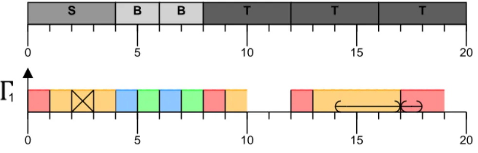
dependency graph of tasks. An example of a schedule over 20 time units is shown in Figure 5. Notice that the schedule of tasks in Figure 5 is the same as the schedule of frames in Figure 3.

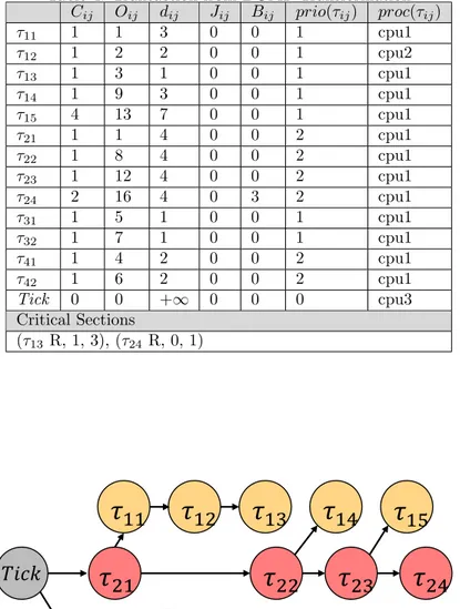
Table 4: Transaction from DGMF Transformation Cij Oij dij Jij Bij prio(τij) proc(τij) τ11 1 1 3 0 0 1 cpu1 τ12 1 2 2 0 0 1 cpu2 τ13 1 3 1 0 0 1 cpu1 τ14 1 9 3 0 0 1 cpu1 τ15 4 13 7 0 0 1 cpu1 τ21 1 1 4 0 0 2 cpu1 τ22 1 8 4 0 0 2 cpu1 τ23 1 12 4 0 0 2 cpu1 τ24 2 16 4 0 3 2 cpu1 τ31 1 5 1 0 0 1 cpu1 τ32 1 7 1 0 0 1 cpu1 τ41 1 4 2 0 0 2 cpu1 τ42 1 6 2 0 0 2 cpu1 Tick 0 0 +∞ 0 0 0 cpu3 Critical Sections (τ13 R, 1, 3), (τ24 R, 0, 1)

𝑇𝑖𝑐𝑘

𝜏

₁₁

𝜏

₁₄

𝜏

₁₅

𝜏

₂₁

𝜏

₂₂

𝜏

₂₃

𝜏

₂₄

𝜏

₃₁

𝜏

₃₂

𝜏

₄₁

𝜏

₄₂

𝜏

₁₂

𝜏

₁₃

0 5 10 15 20

S B B T T T

TDMA Frame

1

0 5 10 15 20

Figure 5: Transaction from DGMF Tasks Transformation: Curved arrows are shared resource critical sections; Tasks execute on same processor except the crossed task

Task Tick represents a ghost root task (defined below) to simplify the anal-ysis, as proposed by [8]. In the specific example, Tick can represent the first TDMA tick that starts the whole TDMA frame. Therefore the ghost root task ensures that all tasks, constrained by the TDMA frame, are part of the same precedence dependency graph. For completeness, parameters of Tick are also given in Table 4. Conform to its definition, Tick is allocated alone on a proces-sor (cpu3 ). It has an execution time of 0, and offset of 0, an infinity deadline, no jitter, a blocking time of 0, and its priority does not matter since it is allocated alone on cpu3.

Definition 2 (Ghost Root Task). A ghost task is allocated alone on a processor and is modeled only for the purpose of the analysis. It has a BCET and WCET of 0, an offset of 0, an infinity deadline, no jitter, a WCBT of 0, and its priority does not matter since it is allocated alone on a processor. In a transaction, a ghost root task is a ghost task that precedes all other tasks, and does not have any predecessor.

The next section determines the characteristics of the transaction given by the transformation example presented in this section, and in the general case. A suitable schedulability test is also discussed.

4.2.4 Assessing Schedulability of Resulting Transactions

The task parameters in Table 4, the precedence dependency graph in Figure 4, and the schedule in Figure 5 show that the transaction presented in the last section has the following characteristics:

• Tree-shaped

Definition 3 (Non-Immediateness). A task τixand its immediate successor task

τiy are said to be non-immediate tasks if τix= pred(τiy)∧Oiy> Oix+Cixb . Task

τix is called a non-immediate predecessor and τiy a non-immediate successor.

A non-immediate task is thus one that is not necessarily immediately released by its predecessor. It is released at an earliest time t if the predecessor completes before or at t, but immediately by the predecessor if the predecessor completes after t.

In the general case, tree-shaped transactions with non-immediate tasks are the results of the DGMF to transaction transformation, if the DGMF tasks set has the Unique Predecessor property:

Theorem 1. A DGMF tasks set with the Unique Predecessor property (Property 1) is transformed into a transaction set without tasks that have more than one predecessor.

Proof. Let a DGMF tasks set have the Unique Predecessor property. A frame F_ij with inter and intra-dependencies is transformed into a task τij with several

immediate predecessors. Task τij has several immediate predecessors that

cor-respond to predecessor frames of F_ij. Let τiy be an immediate predecessor of

τij.

Algorithm 4.2.2.5 removes the precedence dependency τiy ≺ τij, if it is

re-dundant, i.e. if τiydoes not result from a frame in the reduced set of predecessors

(see Property 1) of F_ij. From now, let us consider that redundant precedence dependencies have been removed. Otherwise said, only frames of the reduced set of predecessors of F_ij are considered, as well as tasks that result from them.

At most one predecessor frame Fy

x of F

j

i can have a global deadline (i.e.

ry

x+ Dyx) greater than the release time r j i of F

j

i. By construction, at most one

immediate predecessor τiy of τij (resulting from Fxy and assigned to the same

transaction as τij) can have a global deadline greater than the offset of τij (i.e.

Oiy+ diy ≥ Oij). Algorithm 4.2.2.5 removes a precedence dependency τiy≺ τij

if Oij > Oiy+ diy. Since there is at most one immediate predecessor τiy of τij

that has Oiy+ diy ≥ Oij, all other immediate predecessors will be reduced until

task τij has at most one immediate predecessor.

This proves that tree-shaped transactions result from transformation of DGMF tasks respecting the Unique Predecessor property. The transformation example in Section 4.2.3 showed that there is at least one case where there are non-immediate tasks in the transactions set resulting from the transformation.

To assess schedulability of transactions that are the result of the transfor-mation, a schedulability test applicable to tree-shaped transactions with non-immediate tasks must be applied. This section (Section 4) does not focus on proposing a schedulability test for tree-shaped transactions with non-immediate tasks. The test will be the subject of Section 5.

Furthermore, without knowledge that the tasks represent frames initially, the schedulability test considers that it is possible for job k of a task τi1representing

representing the last frame of the same DGMF task Gi. In practice, this is not

possible because job k of τi1 executes after job τiNi because frames represent

jobs of a DGMF task. If the Cycle Separation property is met, then job k of τi1

will only interfere job k − 1 of τiNi if τiNi misses its deadline. This is why the

Cycle Separation property is assumed.

The following section shows some experiments that evaluate the DGMF modeling and the transformation of DGMF tasks to transactions.

4.3

Experiment and Evaluation

The DGMF scheduling analysis method is implemented in the Cheddar schedul-ing analysis tool. Therefore the DGMF and GMF task models, transaction model, transformation of DGMF tasks to transactions, and some schedulability tests for transactions are implemented in this tool1.

In this section, three aspects of the DGMF to transaction transformation are evaluated through experiments. The following sections first evaluates the transformation correctness, then the transformation time performance, and fi-nally the DGMF modeling and transformation scalability, when it is applied to a real case-study.

4.3.1 Transformation Correctness

The transformation correctness is evaluated by scheduling simulation performed on randomly generated system architecture models. Cheddar provides a module that is able to generate random architecture models. The generator is updated so DGMF tasks can be produced.

The generator respects some parameters defined by the user. The user may define the number of entities in the model, i.e. processors, DGMF tasks, frames, shared resources, critical sections, and precedence dependencies. The user may also define the scheduling policy, the number of DGMF tasks with the same GMF period (called ”synced DGMF tasks”), and the GMF period for such tasks. The generator avoids inconsistencies in the model (e.g. DGMF tasks with no frames). It also produces precedence dependencies in a way that avoids deadlocks during the scheduling simulation.

By using an architecture generator of Cheddar, DGMF task sets are ran-domly generated. The varying generator parameters are: 2 to 5 DGMF tasks, as many frames as tasks and up to 10 for each number of tasks, 1 to 3 shared resources, as many critical sections as frames, as many precedence dependen-cies as frames, a GMF Period between 10 to 50, and 50% of DGMF tasks with the same GMF Period. From these parameters, 540 DGMF architecture mod-els are generated. Each of them is transformed to an architecture model with transactions.

1_{All sources available at http://beru.univ-brest.fr/svn/CHEDDAR/trunk/src/;} Exam-ples of use available at http://beru.univ-brest.fr/svn/CHEDDAR/trunk/project_examExam-ples/ dgmf_sim/ and http://beru.univ-brest.fr/svn/CHEDDAR/trunk/project_examples/ wcdops+_nimp/

The number of tasks, critical sections, and precedence dependencies in the transaction models are equal to the number of frames, critical sections, and precedence dependencies in the DGMF models. The number of output trans-actions is less than the number of input DGMF tasks, since some transtrans-actions are merged into a same one, during the transformation.

Both DGMF and transaction models are then simulated in the feasibility interval proposed in [31]. Schedules are then compared. Each DGMF schedule is strictly similar to the corresponding transaction schedule. Along with the proofs in Section 4.2.2, this experiment enforces the transformation correctness and its implementation correctness in Cheddar.

4.3.2 Transformation Time Performance

In the Cheddar implementation, the time complexity of the transformation al-gorithm depends on two parameters: nF the number of frames, and nD the

number of task dependencies (both precedence and shared resource). The com-plexity of the transformation is O(n2

D+nF). When nF is the varying parameter,

the complexity of the algorithm should be O(nF). When nD is the varying

pa-rameter, the complexity of the algorithm should be O(n2

D) due to Algorithm

4.2.2.2, which has the same complexity as the algorithm in [22]. The experiment in this section checks that the duration of the transformation, implemented in Cheddar, is consistent with these time complexities. Measurements presented below are taken on a Intel Core i5 @ 2.40 GHz processor.

Figure 6 shows the transformation duration by the number of frames. The number of precedence dependencies is set to 0 (i.e. no intra-dependencies either). Figure 6 shows that the duration is polynomial when the number of frames varies. One can think that this result is inconsistent with the time complexity of the algorithm, which should be O(nF) when nF is the varying parameter. In

practice, the implementation in Cheddar introduces a loop to verify that a task is not already present in the system’s tasks set. Thus the time complexity of the implementation is O(n2

F).

Figure 7 shows the transformation duration by the number of precedence de-pendencies. The number of frames is set to 1000, the number of DGMF tasks to 100, and the number of shared resources to 0. In the Cheddar implementation it does not matter which dependency parameter (precedence or shared resource) varies to verify the impact of nD. Indeed, all dependencies are iterated through

once and precedence dependency has more impact on the transformation dura-tion. Since there are 1000 frames and 100 DGMF tasks, the minimum number of precedence dependencies starts at 900, due to intra-dependencies.

The transformation duration should be polynomial when the number of precedence dependencies vary but this can not be noticed in Figure 7 due to the scale of the figure. Indeed, there is already a high minimum number of precedence dependencies starting at 900. The local minimum of the polynomial curve is at 0, like in Figure 6. The curve is a polynomial curve and the re-sult is consistent with the complexity, which is O(n2_D) when nD is the varying

0 200 400 600 800 1000

Frames

T

ime (ms)

Figure 6: Transformation Duration by Number of Frames

1000 1100 1200 Precedence Dependencies 110 120 130 140 150 160 T ime (ms)

Overall a system with no dependency, 1000 frames, and 100 DGMF tasks, takes about 120 ms to be transformed on the computer used for the experiment. A system with 1100 precedence dependencies, 1000 frames, and 100 DGMF tasks, takes less than 160 ms to be transformed. The transformation duration is acceptable for Thales. Indeed, a typical Thales system has 10 tasks and a TDMA frame of 14 slots (1 S, 5 B, 8 T). There would be a maximum of 140 frames (14 × 10), and 256 precedence dependencies (10 × 14 − 10 + 9 × 14) if all tasks are part of a same precedence dependency graph, where a task releases at most one task, and a first task is released at each slot.

4.3.3 Case-Study Modeling with DGMF

The scalability of the DGMF task model, and its transformation to transaction, is assessed by applying DGMF for the modeling of a real software radio protocol developed at Thales. The case-study is implemented with 8 POSIX threads [32] on a processor called GPP1, and 4 threads on a processor called GPP2. The threads are scheduled by the SCHED FIFO scheduler of Linux (preemptive FP policy). The threads have precedence dependencies, whether they are on the same processor or not. For example threads on GPP1 may make blocking calls to functions handled by threads on GPP2. When a thread makes a blocking call to a function, it has to wait for the return of the function, before continuing execution. There is one thread on GPP2 dedicated to each thread on GPP1 that may make a blocking call.

The TDMA frame of the case-study has 1 S slot, 5 B slots, and 8 T slots. The threads are released at different slots. The release logic is a thread dedicated to reception is released at a Rx slot, while a thread dedicated to transmission is released so its deadline coincides with the start of a Tx slot.

In total, there are 36 jobs from 8 threads on GPP1, and 4 threads on GPP2. The threads, their precedence dependencies, and the time parameters of their jobs are illustrated in Figure 8.

The case-study is modeled with a DGMF task model of 43 frames. There are more frames than the 36 jobs because some jobs that make a blocking call to a function, are divided into several frames. After the transformation, a transaction of 44 tasks is the result. The extra task, compared to the 43 frames, is a ghost root task added by a test like [8]. The transaction is illustrated in Figure 9.

Notice that different jobs of a thread, released at different slots, become non-immediate tasks in the transaction, related by precedence dependency (e.g. RS B1 ≺ RS B2 ). Furthermore, a thread that makes a blocking call, to a function handled by a thread on GPP2, is divided into several frames, and then several tasks (e.g. Frame Cycle becomes FC S1 1 ≺ FC S1 2 ≺ FC S1 3 ).

Furthermore, it may seem that some tasks should have two predecessors. For example we should have AB B1 1 ≺ AB B2 1 because these two tasks represent two jobs of a same thread. We should also have Rx Slot B2 ≺ AB B2 1 since these two tasks represent jobs of two threads with a precedence dependency. But since the offset of AB B2 1 is strictly greater than the deadline of Rx Slot B2,

S1 B1 B2 B3 B4 B5 T1 T2 T3 T4 T5 T6 T7 T8 Frame_Cycle Req_Msg Build_TSlot Build_SSlot Build_BSlot Deadline in next frame Deadline in next frame Rx_Slot Analyse_Beacon Analyse_Data Tx Rx Rx Rx Rx Tx Tx Rx Tx Rx Tx Rx Tx Rx

Figure 8: TDMA Frame and Threads of Real Case-Study: Line = Instances of a thread; Down arrow = Deadline; Dashed arrow = Precedence; Black = Exec on GPP1 ; Gray = Exec on GPP2 ; 36 jobs in total from 8 threads on GPP1 and 4 threads on GPP2 ; Sizes not proportional to time values

RM_T1 RM_T3 FC_S1_1 RM_T5 RM_S1 RM_T7 RM_B5 BT_T1 BB_B5_1 BB_B5_2 BB_B5_3 BT_T3 BT_T5 BT_T7 RS_B1 RS_B2 RS_B3 RS_B4 RS_T2 RS_T4 RS_T6 RS_T8

AD_T2 AD_T4 AD_T6 AD_T8 AB_B1_1 AB_B1_2 AB_B1_3 AB_B2_1 AB_B2_2 AB_B2_3 AB_B3_1 AB_B3_2 AB_B3_3 AB_B4_1 AB_B4_2 AB_B4_3 Tick BB_S1_1 BB_S1_2 BB_S1_3 FC_S1_2 FC_S1_3

Figure 9: Tree-Shaped Transaction of a Real Case-Study: Black tasks on GPP1, gray tasks on GPP2, Tick task is ghost root task; Task nomenclature is [Name] [Slot] [Part (Optional)]; Abbreviated names are RM = Request Msg, BT = Build TSlot, BB = Build BSlot, BS = Build SSlot, FC = Frame Cycle, RS = Rx Slot, AB = Analyse Beacon, AD = Analyse Data