HAL Id: hal-02013421
https://hal.inria.fr/hal-02013421
Submitted on 20 Mar 2019
HAL is a multi-disciplinary open access
archive for the deposit and dissemination of
sci-entific research documents, whether they are
pub-lished or not. The documents may come from
teaching and research institutions in France or
abroad, or from public or private research centers.
L’archive ouverte pluridisciplinaire HAL, est
destinée au dépôt et à la diffusion de documents
scientifiques de niveau recherche, publiés ou non,
émanant des établissements d’enseignement et de
recherche français ou étrangers, des laboratoires
publics ou privés.
Modeling SSD I/O Performance for Container-based
Virtualization
Jean-Emile Dartois, Jalil Boukhobza, Anas Knefati, Olivier Barais
To cite this version:
Jean-Emile Dartois, Jalil Boukhobza, Anas Knefati, Olivier Barais. Investigating Machine Learning
Algorithms for Modeling SSD I/O Performance for Container-based Virtualization. IEEE transactions
on cloud computing, IEEE, 2019, 14, pp.1-14. �10.1109/TCC.2019.2898192�. �hal-02013421�
Investigating Machine Learning Algorithms for
Modeling SSD I/O Performance for
Container-based Virtualization
Jean-Emile Dartois, Jalil Boukhobza, Anas Knefati and Olivier Barais
Abstract—One of the cornerstones of the cloud provider business is to reduce hardware resources cost by maximizing their utilization. This is done through smartly sharing pro-cessor, memory, network and storage, while fully satisfying SLOs negotiated with customers. For the storage part, while SSDs are increasingly deployed in data centers mainly for their performance and energy efficiency, their internal mech-anisms may cause a dramatic SLO violation. In effect, we measured that I/O interference may induce a 10x performance drop. We are building a framework based on autonomic computing which aims to achieve intelligent container place-ment on storage systems by preventing bad I/O interference scenarios. One prerequisite to such a framework is to design SSD performance models that take into account interactions between running processes/containers, the operating system and the SSD. These interactions are complex. In this paper, we investigate the use of machine learning for building such models in a container based Cloud environment. We have investigated five popular machine learning algorithms along with six different I/O intensive applications and benchmarks. We analyzed the prediction accuracy, the learning curve, the feature importance and the training time of the tested algorithms on four different SSD models. Beyond describing modeling component of our framework, this paper aims to provide insights for cloud providers to implement SLO compliant container placement algorithms on SSDs. Our machine learning-based framework succeeded in modeling I/O interference with a median Normalized Root-Mean-Square Error (NRMSE) of 2.5%.
Index Terms—Cloud Computing, Performance and QoS, I/O Interference, Solid State Drives, flash memory, Container, Machine Learning
I. Introduction
Companies are increasingly turning to cloud comput-ing services for hostcomput-ing their applications in order to reduce their Total Cost of Ownership (TCO) and increase their flexibility [42]. In this domain, container adoption is growing and Docker [45] is one of the most popular technologies used: three years ago, Docker had about 3% market share, but by 2017 it was running on 15% of the hosts [1]. Containers are used in private and public J.Dartois, J.Boukhobza, Anas Knefati and Olivier Barais are with IRT b<>com.
J.Dartois and O.Barais are also with Univ Rennes, Inria, CNRS, IRISA.
J.Boukhobza is also with Univ. Bretagne Occidentale. Contact: [email protected]
clouds such as OVH 1, Microsoft Azure and Google Compute Engine.
In a container-based system, applications run in isola-tion and without relying on a separate operating system, thus saving large amounts of hardware resources. Re-source reservation is managed at the operating system level. For example, in Docker, Service Level Objectives (SLOs) are enforced through resource isolation features of the Linux kernel such as cgroup [44].
Efficiently sharing resources in such environments is challenging in order to ensure SLOs. Several studies have shown that, among the shared resources, I/Os are the main bottleneck [3], [29], [54], [54], [60], [60], [71], [72]. As a consequence, Solid State Drives (SSDs) were massively adopted in cloud infrastructure to provide better per-formance. However, they suffer from high performance variations due to their internals and/or on the applied workloads.
We define three types of I/O interferences on a given application I/O workload in SSD based storage systems. First, an I/O workload may suffer interference due to SSD internal mechanisms such as Garbage Collection (GC), mapping, and wear leveling [30]. We have mea-sured that, for a given I/O workload, depending on the SSD initial state, the performance can dramatically drop by a factor of 5 to 11 on different SSDs because of the GC (see Section II-D). Second, an application I/O workload may also undergo I/O interference related to the ker-nel I/O software stack such as page cache read-ahead, and I/O scheduling. For instance, in [63], the authors showed that by using different I/O schedulers (CFQ and deadline) on two applications running in isolation, the throughput may drop by a factor of 2. Finally, the workload may also suffer I/O interference related to a neighbor application’s workload. For instance, workload combination running within containers may decrease the I/O performance by up to 38% [71].
Many studies have been conducted to tackle I/O in-terference issues [58], [74]. These solutions are mainly preventive and are designed at different levels. At the device level, the authors of [36], [37] have proposed optimizations related to SSD algorithms and structure such as isolating VMs on different chips. Unfortunately, to the best of our knowledge, this type of SSD is not
commercialized and no standard implementation is pro-posed. At the system level, some studies [3], [63] have attempted to modify the I/O scheduler and the Linux cgroup I/O throttling policy. Finally, at the application level, in [48], the authors presented an approach for modeling I/O interference that is closely related to ours. However, the authors focused on HDDs and did not consider SSDs and their specific I/O interferences.
We are designing a framework to enable container placement in a heterogeneous cloud infrastructure to satisfy users SLO and avoid I/O performance issues related to above-mentioned interferences for SSDs. This framework relies on a self-adaptive autonomic loop. It is mainly based on two components, a first component that monitors container I/Os, and analyzes the I/O patterns and a second component that relies on I/O performance models to decide about the container placement and executes the issued plan that will fully satisfy user requirements by avoiding bad I/O interference. A crucial part in such a framework is the I/O performance models that are used by the planner. This paper mainly focuses in designing these models.
In this paper, we present the investigations achieved about the use of machine learning for building pre-dictive I/O performance models on SSDs in order to anticipate I/O interference issues in container based clouds. We evaluated five learning algorithms based on their popularity, computational overhead, tuning dif-ficulty, robustness to outliers, and accuracy: Decision Trees (DT), Multivariate Adaptive Regression Splines (MARS), Adaptive Boosting (AdaBoost), Gradient Boost-ing Decision Tree (GBDT), and Random Forest (RF). Finding the adequate algorithm for modeling a given phenomenon is a challenging task which can hardly be achieved prior to investigation on real data. Indeed, the relevance of the chosen algorithm depends on several criteria such as the size, the quality or the nature of the modeled phenomenon. We have investigated six I/O-intensive applications: multimedia processing, file server, data mining, email server, software development and web application. The used dataset represents about 16 hours of pure I/Os (removing I/O timeouts) on each of the four tested SSD. We evaluated the relevance of the tested algorithms based on the following metrics: prediction accuracy, model robustness, learning curve, feature importance, and training time. We share our experience and give some insights about the use of machine learning algorithms for modeling I/O behavior on SSDs.
The remainder of the paper is organized as fol-lows. Section II presents some background knowledge. Then, our methodology is described in Section III. Sec-tion IV details the experimental evaluaSec-tion performed. Section V discusses some limitations of our approach. Section VI reviews related work. Finally, we conclude in Section VII.
II. Background and motivation
This section gives some background on SSDs, container-based virtualization and Machine learning. Then, we motivate about the relevance of our study with regard to I/O interference.
A. SSD internals and performance
The main flash memory constraints that affect SSD internals mechanism design is the erase-before-write rule and the limited number of erase cycles a flash memory cell can sustain [10]. In effect, a page cannot be updated without prior erase operation. Data updates are performed out-of-place with a mapping scheme to keep track of data position. These mapping schemes are different from one SSD to another and may induce large performance differences. Out-of-place updates also make it necessary to have garbage collection (GC) mechanisms to recycle previously invalidated pages. GC also have a great impact on performance, especially in case of bursts of random writes as those operations delay application I/O request completion. On the other hand, the limited lifetime of flash memory cells makes it crucial to use wear
leveling techniques. In addition, SSDs make use of paral-lelism within flash chips/dies/planes through advanced
commands in order to maximize the throughput. The complexity of SSD architectures and their wide design space have two major impacts with respect to per-formance. First, the performance may vary dramatically from one SSD to another, and second, for a given SSD, performance also varies according to the interaction of a given I/O workload, with other workloads, with system related mechanisms, and with SSD internal mechanisms. These variations may induce a significant impact on SLOs.
B. Container-based I/O Virtualization
Containers are now widely used to modularize each application into a graph of distributed and isolated lightweight services [62]. As a result, each micro-service has the illusion that it owns the physical re-sources, yet the system lets them share objects (e.g., files, pipes, resources).
Docker [45] is generally used as a lightweight con-tainer system. It provides a common way to package and deploy micro-services [20]. The Linux kernel provides the cgroup functionality that makes it possible to limit and prioritize on resource usage (CPU, memory, block I/O, network, etc.) for each container without the need for starting any virtual machine [70]. cgroup provides a specific I/O subsystem named blkio, which sets limits on and from block devices.
Currently two I/O control policies are implemented in
cgroup and available in Docker: (1) a Complete Fairness
Queuing (CFQ) I/O scheduler for a proportional time based division of disk throughput, and (2) a throttling policy used to bound the I/O rate for a given container.
In the case of SSD with a SATA interface, both policies are available. For NVMe [53], only the throttling policy is available. By default, the latest version of Docker (version 17.03.0-ce) uses cgroup v1. In this version, the I/O control only works on synchronous I/O traffic. Unfortunately, most tested applications do not use such I/Os. As a consequence, we cannot properly limit the bandwidth of each container. This limitation is addressed in cgroup v2 but is not yet supported by Docker.
C. A short introduction to Machine learning
Machine learning investigates automatic techniques to make accurate predictions based on past observa-tions [5]. Datasets contain a set of parameters called features, used to build a prediction model for some specific output response metrics. I/O access patterns (random/sequential) and operation types (read/write) are examples of features while the throughput is the output response.
There are three different categories in machine ing: supervised, unsupervised and reinforcement learn-ing. In supervised learning, the algorithm uses features and their corresponding response values in order to model relationships between features and responses. It includes two types of problems, Classification: for cate-gorical response values (e.g., an email is spam or not), and Regression: for continuous-response values (e.g., I/O throughput). In unsupervised learning, the algorithm only relies on the input features as the corresponding responses are not available. The goal is to let the learning algorithm find by itself how data are organized or clus-tered. In reinforcement learning, the algorithm interacts dynamically with its environment in order to reach a given goal such as driving a vehicle.
Our objective in this study is to build a predictive model that detects existing relationships between I/O features (e.g., block size, R/W rate, mixed workloads) and system responses (throughput). As a consequence, our problem fits in the supervised learning category. Since we want to predict SSD throughput which is a continuous value, we used regression-based algorithms.
D. Motivation
We performed some experiments to observe I/O inter-ference due to SSD internals, and neighbor applications. The system configuration used can be found in Section IV-B
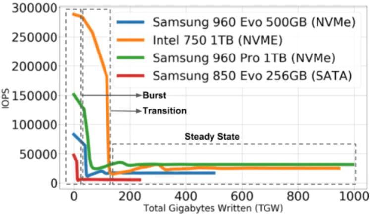
Concerning SSD-related interference, we focused on the SSD initial state impact. In fact, varying the initial state makes it possible to trigger the GC execution. We designed microbenchmarks using fio [6] relying on the Storage Networking Industry Association (SNIA) speci-fication [66]. This specispeci-fication includes a secure erase, a workload-independent preconditioning to attain the so-called SSD Steady State. We performed intensive random writes with a 4KB request size.
Figure 1 shows the measured IOPS. One can observe three states for each device: fresh out of box, transition
Fig. 1. I/O performance of random writes for 4 SSDs
and steady state. More importantly, we can observe from 5x to 11x performance drop when the system sustains continuous bursts of random writes (far below values reported in datasheets). This is due to GC latency as it takes more time to recycle blocks when the volume of free space is low. In reality, the system keeps on oscillating between the three states according to the sustained I/O traffic and the efficiency of the GC.
We have also performed some experiments to identify the I/O interference due to neighbor workloads (on the same SSD). We ran three different containers in parallel and observed the throughput for one specific reference container that runs sequential write operations. For the other two containers, we built up four scenarios ; random write/read, and/or sequential write/read. The volume of generated I/O requests was the same for each experiment. As described in Section II, cgroup v1 cannot limit properly asynchronous I/O traffic. So, containers were not bound by cgroup in terms of I/O performance. Figure 2 shows the performance of the reference con-tainer for the four scenarios on four different SSDs. We observe that the performance drop between the maximum and minimum throughput obtained for the reference container represents 22% in the best case (SATA disk with which CFQ can be used) and up to 68% in the worst case with a small dispersion (i.e., an interquartile range of 0.04125 in case of the Evo 850 SSD for two executions). This value represents the variation due to the neighboring containers only.
As a consequence, placing a set of containers on a set of SSDs is a real issue that needs to be investigated to avoid high SLO violations.
To conclude, we have illustrated two types of I/O in-terference, first the sensitivity to the write history which induces I/O interaction with the GC (SSD internals), and second the I/O interactions between I/O workloads which may strongly impact the performance. This moti-vated us to investigate ways to model I/O throughput taking into account these interactions in order to avoid SLO violations.
Fig. 2. I/O Interference of mixed workloads
III. Modeling SSD I/O performance: a machine learning approach
A. Overall project
Fig. 3. Overall project
We seek at developing a framework to enable container placement in a heterogeneous cloud infrastructure in order to satisfy users SLO and avoid I/O performance glitches.
To achieve this, we devise a self-adaptive
container-based MAPE-K
(Monitor-Analyze-Plan-Execute-Knowledge) [35] loop, an extensively used reference architecture for cloud computing optimization [43], [49], [51] (like the OpenStack Watcher project we have previously developed 2 that was specific to virtual machines).
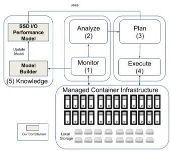
The MAPE-K loop is composed of four main steps depicted in Figure 3:
1) Monitor: our framework collects containers’ I/O requests using a previously designed block-level I/O tracer3.
2http://github.com/openstack/watcher 3https://github.com/b-com/iotracer
2) Analyze: containers’ I/O traces are continuously analyzed and preprocessed for the next step. 3) Plan: the framework relies on one hand on the
containers I/O patterns from the analyze step and current containers placement, and on the other hand on the I/O SSD performance model (see the knowledge part) in order to issue a container placement plan. This performance model is up-dated continuously when needed according to the monitored I/Os. This may be done either by per-forming Online learning or by updating the model whenever new applications (new I/O interferences) are run or new storage devices are plugged in. 4) Execute: the proposed container placement is
scheduled and executed on the real system by calling the adequate APIs of the used infrastructure manager, such as Kubertenes [33].
5) Knowledge: in our framework, the knowledge part is related to the SSD I/O performance model built and that drives the overall placement strategy (of the plan phase).
This paper focuses on the Knowledge part of the loop. The SSD I/O performance models are built thanks to the Model builder component that relies on machine learning algorithms. This paper details our methodology for designing such a component and gives a return of experience about our investigations.
B. Approach scope and overview
To build a predictive model that is able to forecast SSD I/O performance in container-based virtualization environment, one needs to fix the scope of the model. From the application point of view, we used six data-intensive applications and a micro-benchmark: video processing, file server, data mining, email server, soft-ware development and web application, this is detailed in Section III-C. From a system point of view, our study does not focus on I/O variations related to system configuration change (such as read-ahead prefetching window size or I/O scheduler). System related parame-ters (e.g., kernel version, filesystem, docker version, etc.) were fixed for our experiments and are detailed in the Evaluation section. Finally, from the storage device point of view, we have experimented with 4 SSD models, both SATA and NVMe, to explore the difference in predictive models as compared to the used technology/interface.
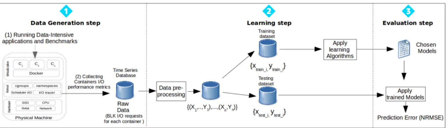
Figure 4 describes the overall approach followed with three different steps:
• Dataset generation step: A challenge in model
build-ing is to use representative data to build an accurate predictive model. In our study, we created datasets by monitoring containers running real applications and benchmarks, see Section III-C.
• Learning step: we built the I/O performance model
based on a subset of collected I/O traces/data (supervised learning) using five machine learning algorithms discussed in Section III-D. In the learning
step, one needs to pre-process the data (I/O traces collected) in order to extract the input features and the responses from the traces. Then, one needs to split the data to decide about the part that will be used to train the model and the one used to evaluate it, see Section III-D
• Evaluation step: In this step, we evaluated the
accu-racy of the trained model, see Section IV.
C. Dataset generation step
In the dataset generation phase, we have mainly two steps (see Figure 4): generating the workload by execut-ing different applications and collectexecut-ing the I/O traces. For the sake of our study, we have generated our own datasets. Indeed, we did not find any dataset available off the shelf that represent typical combinations of I/O requests issued from container environments.
We selected six data intensive applications that were deployed in a container-based environment covering var-ious use-cases and I/O interferences. Those applications behave differently from an I/O point of view. We also used micro-benchmarks as defined by [67] presented in section II-D to generate more I/O interference scenarios. Table II summarizes the benchmarks used.
We used four different scenarios to induce different I/O interferences for the 6 applications:
1) each application was run alone within a container. This was done to determine each application’s performance reference without interference (due to other I/O workloads).
2) up to 5 instances of the same application were run at the same time, each instance was ran within a dedicated container on the same host. This was done in order to generate I/O interference between the same applications. We decided to limit the number of instances to 5 in order to be able to allocate in a fair manner the processor time across the containers. In addition, according to [1] 25% of the companies run less than 4 containers simulta-neously per host with a median of 8 containers. 3) applications were run in a pairwise fashion to test
all possible combinations. This means that with six applications, we executed 15 combinations (e.g., file server with data mining, file server with web application, etc.). This was done to deliberately generate I/O interference per pair between the applications.
4) the six applications were run at the same time in six containers.
These scenarios were executed three times in order to be representative. Additionally to these applications, we used micro-benchmarks to enrich the I/O interference scenarios.
1) Generating workload phase: The used applications
are briefly described per category (see Table II). To generate the dataset, we used the tools Nginx [55], MySQL [47], and WordPress [11] for the web application,
FileBench [65] for the email and fileserver, ffmpeg [7] for the video application, Parsec benchmark suite [8] for the
freqmine application, GNU Compiler Collection [64] for
the compile application.
Server application: We chose three typical enterprise server applications: an n-tiers web application (WordPress), file and email servers (Filebench). WordPress is an Open Source content management system based on Nginx, PHP, and MySQL. In the case of a WordPress website, we varied the number of concurrent readers/writers between 1 and 50. Varying the number of users has a direct impact on the storage system by issuing multiple MySQL connections, and performing multiple table read-s/writes. Moreover, MySQL generates many trans-actions with small random I/O operations. The tool that generates the traffic was run on a separate host. We used Filebench to evaluate email and file servers to generate a mix of open/read/write/close/delete operations of about 10,000 files in about 20 directo-ries performed with 50 threads.
Media processing: ffmpeg is a framework dedicated to audio and video processing. We used two videos, a FullHD (6.3 GB) and an HD (580MB) video. For the transcoding of the H.264 video, we varied the PRESET parameter between slow and ultrafast. This parameter has a direct impact on the quality of the compression as well as on the file size. We encoded up to 5 videos within 5 containers simultaneously. Writing the output video generated a high number of write operations at the device level and may generate erase operations when files are deleted at the end of video transcoding.
Data mining: This application employs an arrays-based version of the FP-growth (Frequent Pattern-growth) method for Frequent itemset Mining. It writes a large volume of data to the storage devices.
Software development: Linux kernel compilation uses thousands of small source files. Its compilation de-mands intensive CPU usage and short intensive random I/O operations to read a large number of source files and write the object files to the disk. For the sake of our study we compiled the Linux kernel 4.2.
2) Collecting Containers I/O metrics: In order to collect
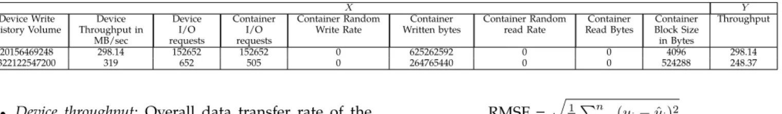
the I/O data, we used a block-level I/O tracer 4 which has a small overhead [50]. It is a kernel module running on the host that automatically detects and monitors new containers I/Os. We chose the block level to build a performance model of the storage system, and so only I/Os satisfied by the SSD were considered. Table I shows a sample of the traced I/O requests. All traced I/Os were inserted in a time series database, see Figure 4.
Fig. 4. Overall Approach
TABLE I
Sample of I/O requests stored in the Time Series Database
Timestamp [milliseconds] Container ID Access Type Address Accessed Data Size [bytes] Access Level 1503293862000 340e0a2d67aa W 83099648 524288 BLK 1503293863000 340e0a2d67aa W 83100672 524288 BLK
TABLE II
Applications and Benchmarks used
Name Category Description
web Server application N-tiers web application
email Server application Email server
fileserver Server application File server
video Multimedia processing H.264 video transcoding
freqmine Data mining Frequent itemset mining
compile Software development Linux kernel compilation
micro-benchmark Synthetic Benchmark I/O workload generator
D. Learning step
Choosing the right learning algorithm for a specific problem is a challenging issue. Many state-of-the-art studies such as [21] have discussed the way to select the appropriate learning algorithm(s) depending on the datasets and the type of problem to solve.
Classical algorithms such as linear discriminant analysis and nearest neighbor techniques, have been criticized on some grounds [13]. For instance, they cannot handle categorical variables and missing data. Other algorithms such as support vector machines depend on the careful selection of hyperparameters and the implementation details [32]. Neural networks suffer from higher compu-tational burden, proneness to over-fitting, the empirical nature of the model development, and the fact that they are hard to debug [68]. In [27], the authors described characteristics of different learning algorithms that we have summarized in Table III, we extracted a list of five algorithms that could fit our needs.
In addition to the prediction accuracy criteria, we selected these five algorithms based on the following criteria:
• Robustness to outliers: In storage systems, we are
concerned about outliers as on average most of I/O requests do not use the whole available performance
TABLE III
Some characteristics of the learning methods used. Key: N= good, ◦=fair, and H=poor.
Characteristic DT MARS AdaBoost GBDT RF
Robustness to outliers N H ◦ N N
in input space
Handling of missing values N N N N N Computational complexity N N H H H
Prediction accuracy H ◦ N N N
of the devices.
• Handling of missing values: The large number of
possible combinations of I/O workloads require a learning algorithms that can handle missing values.
• Computational complexity: We cannot train the
al-gorithms on every combinations once and for all, so we need to be able to recompute the model quickly online to reduce the number of SLA violations.
1) The learning algorithms used: For convenience, we
used the following notation:
• Inputs (features) xi (i = 1, 2, ..., n) is a vector of 9 variables influencing the I/O performance (where n is the total number of data samples available), see Section III-D2 for more details about the feature selection.
• Responses yi (i = 1, 2, ..., n) is the measured perfor-mance in term of throughput.
• Hyperparameters : The accuracy of a model
de-pends strongly on the dataset and the learning algorithm used. It also depends on the algorithm tuning parameters, called hyperparameters. These parameters impact the complexity of the learning model, and they are estimated so as to minimize the error.
We evaluated two methods in order to configure the hyperparameters. The first one consists simply of
us-ing the configuration recommended by the authors (of the algorithm) when available. The second one consists of using the K-fold cross-validation method [40]. Then we chose the configuration giving the best prediction.
The idea of the K-fold cross-validation method is to divide the training set into K roughly equal-sized parts. For the kth (k = 1, ..., K) part, we fit the model to the other K − 1 parts and calculate the prediction error of the fitted model. We combine the K estimates of prediction error.fˆ−kdenotes the fitted model (for k = 1, ..., K), the cross validation estimate of the error is:
CV ( ˆf−k) = 1 K K X k=1 X i∈kthpart (yi− ˆf−k(xi))2 (1)
So, the hyperparameters of the model fˆ−k are es-timated such as to minimize the criterion (1). We used for our simulations K = 5 which is the value recommended in [14].
In what follows, we will describe each of the five ma-chine learning algorithms used and give some elements about hyperparameters configuration.
Decision trees (DT) This method was developed at the University of Michigan by Morgan et al. in the early 1960s and 1970s ( [22], [46]). DT partitions the feature space into a set of rectangles, and then fits a simple model in each one. In this study, we used the method CART (Classification and Regression Trees) [13] which is a popular method in decision trees. It encodes a set of if-then-else rules in a binary tree which are used to predict output variables given the data features. These if-then-else rules are created using the training data which aims to maximize the data separation based on a loss function related to classification or regression scores.
CART method can be evaluated as a linear combi-nation of the indicator function of sub-regions Rm
that form a partition of the feature space: f (x) =
M
X
m=1
cmI(x ∈ Rm), (2)
where I is the indicator function having 1 for x of Rm and 0 for x not in Rm. The weights cm
and the regions Rm are learned from data such as to minimize the loss function. M is the maximum depth of the tree. We increase M such that the nodes are expanded until all leaves contain less than a certain minimum number of samples (5 in our simulations). The DT is composed of two main stages, creating a tree to learn from all the training samples and then pruning it to remove sections that are non significant variables that would decrease the accuracy.
Multivariate adaptive regression splines (MARS) This method was introduced by Friedman [26], it can
be viewed as a generalization of stepwise linear regression or a modification of the CART method to improve its performance in the regression. MARS uses expansions in a piecewise linear basis functions of the form max(0, x − t) and max(0, t − x).
MARS model has the following form:
f (x) = c0+ M
X
m=1
cmhm(x), (3)
where hm(x) (m = 1, ..., m) takes one of the
follow-ing two forms:
• a spline function that has the form
max(0, xi − t) or max(0, t − xi), where xi is a feature and t is an observation of xi. MARS automatically selects xi and t.
• a product of two or more spline functions.
To build the model (in Equation 3), we have two main phases: First, the forward phase is performed on the training set, starting initially with c0. Then, for each stage, the basis pair which minimizes the training error is added to a set M. Considering a current model with m basis functions, the next pair added to the model has the form:
cm+1h`(x) max(0, xi− t) + cm+2h`(x) max(0, t − xi),
where h` ∈ M. Each cm is estimated by the least-squares method. This process of adding basis func-tions continues until the model reaches the maxi-mum number (M ) fixed. Finally, the backward phase improves the model by removing the less significant terms until it finds the best model. Model sub-sets are compared using the less computationally expensive method of Generalized Cross-Validation (GCV ). This criterion is defined as:
GCV = 1 1 −r+0.5d(r+1)N N X i=1 (yi− ˆf (xi)) (4)
in which r is the number of basis functions, d is a penalty for each basis function included in the developed sub-model, N is the number of training datasets, and f (xi) denotes the MARS predicted
values.
In our simulation, we used the penalty d = 3 which is recommended by Friedman [26]. For each deletion step, a basis function is pruned to minimize Equation 4, until the best model is found.
Boosting Methods The basic idea of these methods is that they combine the outputs of many ”weak” estimator into a single estimator that, hopefully, will be much more accurate than any of the ”weak” ones. A weak estimator is one whose error rate is only slightly better than random guessing. Freund and Schapire [23] proposed the most popular boosting algorithm for a binary classification problem which is called AdaBoost.M1 . Zhu et al. [75] extended this algorithm to the multi-class case without reducing
it to multiple two-class problems. Drucker [18] ex-tended the AdaBoost algorithm to regression prob-lems which is the algorithm used in our study. In AdaBoost, the weak learners are decision trees with a single split, called decision stumps. The adaboost model for regression (adaboost.R) has the form:
f (x) = weighted median{ht(x), t = 1, ..., T } (5) where htis a weak regression algorithm. adaboost.R uses multiple iterations to produce a stronger rule, the weights adjust themselves to improve the esti-mator performance. The algorithm scales the con-tribution of each regressor by a factor 0 ≤ ν ≤ 1 called the learning rate. There is a trade-off between the number of weak regression machine and the learning rate.
In our simulation we used T = 200 and five fold cross validation to estimate ν.
Gradient boosting Since the analysis of the properties and performance of boosting methods are rather difficult [59], a gradient-descent based formulation of boosting methods were proposed [24], [25] to establish a connection with the statistical model. These methods build the model in a stage-wise fashion like other boosting methods do, and it gen-eralizes them by allowing optimization of an arbi-trary differentiable loss function. Here we used the Gradient Boosting Decision Trees (GBDT) proposed by Friedman [25]. We used the same methodology in adaboost.R to estimate the learning rate and the number of tree regressors in this model.
Random Forests (RF) They were introduced by Breiman [12]. RF are a substantial modification of decision trees that build a large collection of de-correlated trees, and then averages them. They are a combination of tree predictors such that each tree depends on the values of a random vector sampled independently and with the same distribution for all trees in the forest. The performance of RF is very similar to boosting in many problems, and they are simpler to train and tune [31]. This algorithm depends on the number of trees T and on the following parameters for each tree:
• m : The number of features to consider when
looking for the best split;
• nmin : The minimum number of samples re-quired to split an internal node.
In our simulations, we used the following values recommended by [27] : T = 200, nmin = 5 and
m equal to the floor value of p/3, where p is the number of features in the dataset.
2) Data Pre-processing: The goal of the pre-processing
step is to create the matrix of input features noted x and the vector of the observed responses noted y (i.e., throughput) from the I/O traces stored in the time series database.
The observed response y (throughput) is calculated from the captured I/O trace. We need to define a time
window that would represent one data sample to be used by the learning algorithm. The objective is to have a time window during which we correlate I/O activities of every single container with regards to the others. One needs to compromise on the size of this time window. If it is too large, it would capture too many events and I/O interactions, thus the learning phase will lose in precision. A time window that is too small would generate a too large dataset with a large proportion of samples that do not contain relevant information. We chose a middle-ground and used a time window of 10 seconds. We computed the response vector y = (yi)ni=1
as follows: yi= 1 104 X Ti≤t≤Ti+104 dt (6)
where yi is the throughput in MB/s obtained by one container and Ti is the starting time in milliseconds of the monitoring period. The variable i is the number of time windows within a single sampling window.
The selection of the input features x is a key step to build a good predictive model. One needs to consider the variables that have an influence on the I/O perfor-mance for the learning algorithms to find the (hidden) relationships between x and y (see Section II-C). We have selected 9 features listed below based on [48], [66], [71]: As previously discussed, We have three types of I/O interferences that may affect the throughput: (a) interfer-ence due to SSD internals, (b) interferinterfer-ence related to the kernel I/O software stack, and (c) interference due to the co-hosted applications workloads. One needs to extract the features from the traces in order to represent such interferences.
• Interference (a): this interference is related to the
impact of internal mechanisms of SSDs on perfor-mance, especially the GC. The more the SSD sus-tains write operations, the more the GC is initiated, the higher this impact. As a consequence, we chose to capture this feature with the write operations history of the SSD. Indeed, this history gives indi-cations about the state of the SSD.
• Interference (b): As previously mentioned, system
related parameters were fixed in this study. How-ever, as we trace at the block level layer, the impact of the page cache and the I/O scheduler is already taken into account.
• Interference (c): they are inferred from the traces as
we get the performance of each container knowing what the other collocated containers are doing and the overall performance sustained by the SSD. For each yi we computed the corresponding row of xi
that captures the I/O interference as follow:
• Device write history : This feature represents the
cumulative volume of data written on the device in bytes. We used it to capture SSD internal write operations. Indeed, the more the SSD sustains write operations, the more the GC is initiated, the higher the impact on the application I/Os.
TABLE IV
Pre-processed Data, X: Inputs (features) and Y : Output
X Y Device Write History Volume Device Throughput in MB/sec Device I/O requests Container I/O requests Container Random Write Rate Container Written bytes Container Random read Rate Container Read Bytes Container Block Size in Bytes Throughput 20156469248 298.14 152652 152652 0 625262592 0 0 4096 298.14 322122547200 319 652 505 0 264765440 0 0 524288 248.37
• Device throughput: Overall data transfer rate of the
device.
• Device I/O requests: Number of I/O requests satisfied
by a given device.
• Container I/O requests: Number of I/O requests per
second for each running container.
• Container random write rate: Rate of random write
I/O requests for each running container.
• Container written bytes: Number of bytes written for
each running container.
• Container random read rate: Rate of random read I/O
operations for each running container.
• Container read bytes: The number of bytes read for
each running container.
• Container block size distribution: Block size
distribu-tion for each running container.
Table IV shows a sample of the pre-processing result.
3) Data splitting: The aim of Data splitting step is to
divide the data into two distinct datasets, one for training and one for testing purposes.
We randomly used 75% of the data to train our model through the learning algorithms and the remaining 25% were used for validation purpose as recommended by [14]. We ran this selection step 100 times in order to evaluate the robustness of the tested algorithms. The accuracy of the model may change according to the data splitting performed. A robust algorithm is one that provides a good model regardless of the data splitting being performed.
IV. Evaluation
This section describes the results of our experiments. Through this experiment, we try to answer four research questions:
• RQ1: What is the accuracy and the robustness of
the tested algorithms?
• RQ2: How does the accuracy change with regards
to the size of the training dataset (learning curve)?
• RQ3: What are the most important features in
building the model?
• RQ4: What is the training time overhead?
A. Evaluation metric
One of the most common metric to evaluate the quality of a model is the Root Mean Square Error (RMSE):
RMSE = q 1 n Pn i=1(yi− ˆyi)2
Where yi is the measured and ˆyi the modeled through-put. The RMSE indicator penalizes large deviations be-tween predicted values and observed values. In order to be able to compare SSDs with different performance. We used a Normalized Root Mean Square Error (NRMSE), given by:
NRMSE = RMSE
ymax− ymin
B. Experimental setup
All experiments were performed on a server with an Intel(R) Xeon(R) E5-2630 v2 CPU clocked at 2.60GHz with 130GB of RAM. Concerning the storage system, we used four SSDs: one with a SATA interface (Samsung 850
Evo 256GB MLC) and three others with NVMe interfaces
(Intel 750 1.4TB MLC, Samsung 960 Pro 1TB MLC and a
960 Evo 500GB TLC).
We used the Ubuntu 14.04.4 LTS GNU Linux distribu-tion with a kernel version 4.2.0-27. We used the ext4 file system for all the experiments. The virtualization system used was Docker version 1.12.2.
For our tests, we have used the AUFS storage driver for managing Docker image layers. However, each con-tainer mounts a host directory as a data volume on a locally-shared disk for data-intensive workloads. These data volumes are dependent on the filesystem of the underlying host (ext4) which are recommended for I/O-intensive workloads [20]. Finally, all containers get the same proportion of block I/O bandwidth.
We made use of the xgboost [16] version 0.6 and
scikit-learn [52] version 0.18 libraries which provide
state-of-the-arts machine learning algorithms.
C. Datasets characteristics
This section provides an overview of the used datasets characteristics. For each SSD, the dataset is composed of the six data-intensive applications and a micro-benchmark with the different scenarios presented in Section III-C.
At the block level, 75% of the size of the traced I/Os is between 20KB and 110KB with a median of 64KB which represents most of the typical enterprise block sizes according to the SNIA [19]. The read/write ratios of the tested workloads also covered most of the enterprise applications, see Table V.
In addition, we made sure that the volume of the data written to the disks exceeded by far the size of the disks in order to span the different SSD performance states shown in Figure 2.
TABLE V
Measured workload characteristics
Name Read/Write Ratio [%] Seq/Rand Ratio [%] Block Sizes for 80% of I/Os
web 76/24 10/90 8KB, 16KB, 32KB email 10/90 1/99 4KB, 8KB, 12KB, 16KB fileserver 83/17 30/70 4KB, 8KB, 12KB video 40/60 92/8 512KB freqmine 2/98 99/1 4KB, 8KB, 512KB compile 9/91 65/35 4KB, 8KB
D. Prediction accuracy and model robustness
As explained in Section III-D3, we ran each algorithm 100 times by randomly selecting each time 75% of the dataset (comprising all the applications) to build the model and the remaining 25% to evaluate its accuracy. For each execution, we used 6000 training samples each consisting of 10 seconds of workload (more than 16 hours of pure I/Os excluding I/O timeouts). The accuracy is evaluated through the median NRMSE while the robustness is given by the dispersion.
Fig. 5. Box-plot of NRMSE for each algorithm on all SSDs.
Figure 5 shows the boxplots for each learning al-gorithm according to the storage device used. A first observation is that the more accurate models (median NRMSE represented by the red line within each box) were achieved with AdaBoost, GBDT, and RF with an NRMSE median error of about 2.5%.
A second interesting observation is that the ranking of the learning algorithms is the same regardless of the SSD being used. This is a very interesting result that means that different SSD behaviors can be captured with the same
learning algorithms.
A third observation is that AdaBoost, GBDT, and RF also provide a smaller dispersion compared to the other algorithms. Indeed, the models built with those algo-rithms are less sensitive to the data distribution between
the training set and the testing set. This means that the models built with these algorithms are more inclined to be resilient to any I/O pattern change, which is a very interesting property.
Note that RF and DT gave their results with fixed hyperparameters rather than using cross-validation (see Section III-D1).
Overall one can observe that most of the algorithms used provide an NRMSE lower than 5% when using the 6000 training samples.
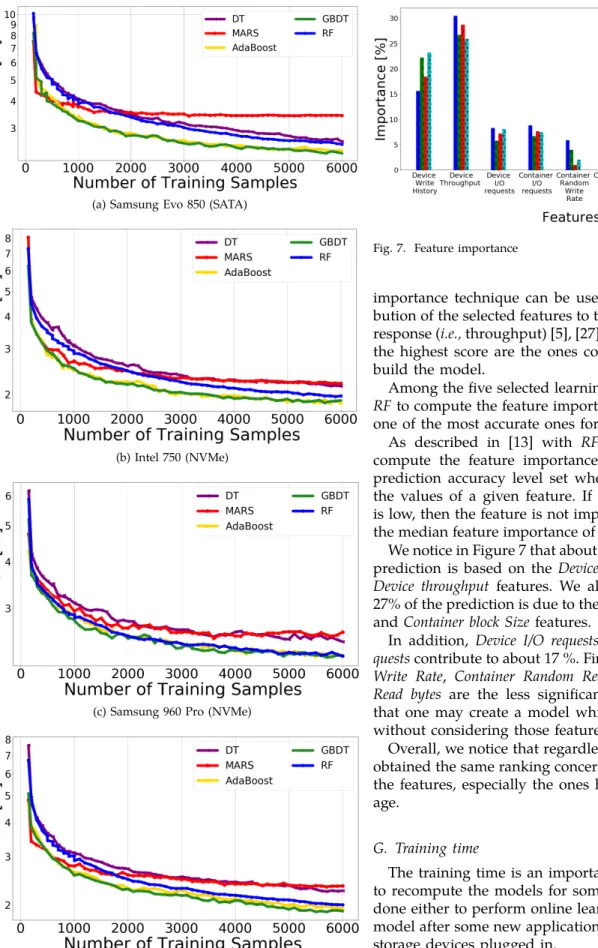
E. Learning curve
The learning curve shows the evolution of the model accuracy (i.e., NRMSE) according to the number of train-ing samples [5], [27].
In order to build our learning curve, we performed a progressive sampling by increasing dataset sizes Ntraining = 150 to Nmax with an increase step of 100 samples (where Nmax is the total number of samples available). At each step, we ran 100 times the algorithm by randomly selecting the data for each iteration. Note that the minimum size of the training set was fixed to 150 samples which is the size recommended in [27] in order to obtain a good performance when using 5-fold cross validation to estimate the hyperparameters.
In Figure 6 we show the accuracy of the algorithms according to the training set size. First, we observe as expected that for each algorithm, the accuracy improves with the increase of the training set size. Second, the best algorithms Adaboost, GBDT and RF have a similar convergence slope. Another interesting result is that the best algorithm ranking is the same for small and large training samples sets used. This ranking corresponds to the one established in the previous section regardless of the used SSD.
Third, we observed that for the first training samples (<1000), the accuracy was not good. This could be explained by the fact that with such a small dataset it is hard to avoid over-fitting but also that the outliers are more difficult to avoid, especially with MARS which is not robust to outliers. We can conclude that we need at least about 3 hours (i.e., about 1100 training samples) of pure I/Os to reach a good level of accuracy.
In a production infrastructure, one may define an off-line SSD warm up period using micro-benchmarks, macro-benchmarks or simply by running target applica-tions on the SSD before integrating the disks into the system. This makes it possible to generate the training samples in order to reach a minimum acceptable accu-racy. In addition, in our study, the model is continuously updated according to the workload using a feedback loop. This allows to continuously refine the learning samples.
F. Feature importance
In this section we want to assess the share of each feature in the model we have developed. The feature
(a) Samsung Evo 850 (SATA)
(b) Intel 750 (NVMe)
(c) Samsung 960 Pro (NVMe)
(d) Samsung 960 Evo (NVMe)
Fig. 6. Learning curves on the testing set as a function of the number of training samples
Fig. 7. Feature importance
importance technique can be used to assess the contri-bution of the selected features to the predictability of the response (i.e., throughput) [5], [27]. The features reaching the highest score are the ones contributing the most to build the model.
Among the five selected learning algorithms, we used
RF to compute the feature importance as it proved to be
one of the most accurate ones for the tested datasets. As described in [13] with RF, one of the ways to compute the feature importance is by measuring the prediction accuracy level set when we randomly swap the values of a given feature. If the accuracy variation is low, then the feature is not important. Figure 7 shows the median feature importance of our predictive models. We notice in Figure 7 that about 46% of the throughput prediction is based on the Device Write History and the
Device throughput features. We also observe that about
27% of the prediction is due to the Container Written bytes and Container block Size features.
In addition, Device I/O requests and Container I/O
re-quests contribute to about 17 %. Finally, Container Random Write Rate, Container Random Read Rate and Container Read bytes are the less significant features.This means
that one may create a model which is accurate enough without considering those features.
Overall, we notice that regardless of the SSD used, we obtained the same ranking concerning the importance of the features, especially the ones having a high percent-age.
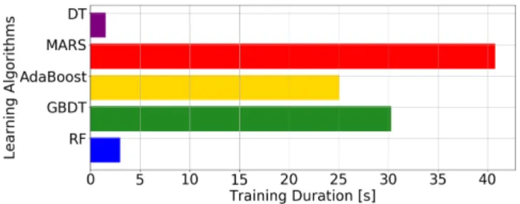
G. Training time
The training time is an important metric if one needs to recompute the models for some reason. This may be done either to perform online learning, or to update the model after some new applications are run or some new storage devices plugged in.
Figure 8 shows the median computation time taken to train each of the five learning algorithms. It turns out that MARS took the longest time for training, with a median time of about 40 seconds (for 6000 training samples). This is due to the complexity of MARS which
Fig. 8. Median computation time used for the training of different learning algorithms
is O(m3), where m is the number of basis functions (see Section III-D1). Then, with a training time of 30 seconds
GBDT is slower than Adaboost (25 seconds). DT and RF
executed in less than 4 seconds.
The duration is highly related to the choice of hyper-parameters (e.g. number of folders in K-cross validation, fixed parameters, etc.).
As compared to the time spent to build the model, the amount of time necessary to make the prediction based on the latter was much shorter (i.e., less than 40
milliseconds).
V. Limitations
There are some potential issues that may have an impact on the results of this study and that could also be considered for future research:
• System parameters such as file system, kernel
ver-sion, prefetching window size, continuous or peri-odic trimming of SSD devices were not varied. These parameters might have an impact on the model building.
• We did not consider CPU and Memory related
metrics in our approach. In [39] authors show that passing from one to two cores may increase the throughput performance from 870K IOPS to 1M IOPS with a local Flash disk. So, these variables may have an impact on I/O performance in case the CPU is overloaded and cannot satisfy I/O requests for instance.
• The used I/O tracer does not monitor file system
metadata [56], this could make our model underes-timate the issued I/Os.
• The size of invalid space in a flash memory may
have an impact on the performance. In addition to the write history, one may use the number of invalid blocks, for example using Smartmontools [4], as a new feature.
VI. Related work
Avoiding I/O interference can be achieved using sev-eral strategies. The first solution is to get a performance model that can capture I/O interference. Another so-lution is to modify the system behavior or the SSD behavior to limit the risk of interference.
Common performance modeling studies have targeted hard drives using analytic modeling [9], [57], [61], sim-ulation [15], [38], benchmarking [2], [67], and black-box approaches [69], [73]. Many analytic and simula-tion approaches were based on understanding internal organization of storage devices. However, the internal design employed by SSDs are often closely-guarded in-tellectual properties [28]. To overcome this issue, black box approaches have been used [34], [69], [73]. In [34], Huang et al. proposed a black box modeling approach to analyze and evaluate SSD performance, including latency, bandwidth, and throughput. In our work, we have included more input features (5 more). In particular, we have included features related to write history and interference between containers, which turned out to be relevant in our work.
To better predict the SSD behavior, some state-of-the-art studies have tried to tackle this problem at different levels, mainly at low level SSD controller and system level. The first class of solutions tries to implement some low level techniques to minimize the interference at the flash memory chip level, for instance by physically storing container data in specific flash chips [37]. My-oungsoo et al [36] proposed to create a host interface that redistributes the GC overheads across non-critical I/O requests. The second class of solutions operates at the system level, Sungyong Ahn et al [3] have modified the Linux cgroup I/O throttling policy by affecting an I/O budget that takes into account the utilization history of each container during a specific time window. The third class of solutions proposes an application-based solution, in [17] and [41] the authors propose to avoid I/O interference by coordinating the applications I/O requests. Noorshames et al. [48] present an approach for modeling I/O interference that is the most closely related to ours. However, the authors focused on HDDs and did not consider SSD-related performance models.
While the first class of solutions is hardly usable for cloud providers using off-the-shelf SSDs, the second ones could be cumbersome to implement and tune for different devices. Our proposed approach complements state-of-the-art solutions and can be used independently from low-level optimizations.
VII. Summary and Perspectives
According to our study, it turned out that Machine learning is a relevant approach to predict SSD I/O performance in a container-based virtualization. We eval-uated five learning algorithms. The features used for the regression were extracted from six data-intensive applications and micro-benchmarks. We experimented with 4 SSDs. We draw several conclusions that may help Cloud providers to design a machine learning based approach to avoid SLO violation due to I/O performance issues:
Prediction accuracy and models robustness (RQ1 Findings):
• GDBT, Adaboost and RF gave the best performance
with an NRMSE of 2.5% using 6000 training sam-ples. From the three algorithms, RF was the most accurate.
• The ranking of the tested algorithms was the same
regardless of the SSD used.
• Adaboost, GDBT and RF provided the smallest
dis-persion proving there robustness to a changing I/O pattern.
• We used fixed hyperparameters to tune RF and DT.
This makes these algorithms simpler to use. Learning curve (RQ2 Findings):
• The prediction accuracy is enhanced for every
algo-rithm as we add more training samples.
• The ranking of the algorithms accuracy remained
the same regardless of the number training samples (RF, GDBT and Adaboost).
• We need at least a dataset of about 3 hours of
pure I/Os to reach a good level of accuracy and a minimum of 150 samples to run the algorithms. Feature Importance (RQ3 Findings):
• The importance of the features was not balanced.
The most important ones were the Device write
history, device throughput, container written bytes and container block size. These features are available off
the shelf. Surprisingly, the random write rate did not prove to be very important.
• The ranking of features importance was the same
for all SSDs, especially the most important ones. Training Time (RQ4 Findings):
• The training time of RF and DT was the shortest
one.
• The training time of all algorithms was small
enough to be used in runtime to update the model. This is a good property if we have to recompute the model for a new device, a new system configuration, or a new I/O pattern.
Predicting I/O performance in container-based virtu-alization is necessary to guarantee SLO. We will use the results of our approach to develop a strategy to improve container placement in cloud infrastructure in order to avoid performance issues before users are impacted.
We also plan to integrate new metrics (e.g., disk la-tency) and also new features to train our model such as the number of invalid blocks, file-system aging, CPU, memory.
We will also work toward considering reinforcement learning to integrate the three steps/modules (i.e., Ana-lyze, Plan, Execute) in the same framework by applying directly new container placement strategy in the Cloud infrastructure in order to maximize a given reward met-ric.
While in this paper we limited the experiments to 5 containers, a perspective could be to add more containers and to evaluate the potential limitations.
Other experiments are also underway to apply the same types of experiments for virtual machines deploy-ment using KVM.
Acknowledgment
This work was supported by the Institute of Research and Technology b-com, dedicated to digital technologies, funded by the French government through the ANR Investment referenced ANR-A0-AIRT-07.
References
[1] 8 surprising facts about real docker adoption, 2016. https://www.datadoghq.com/docker-adoption/.
[2] N. Agrawal, A. C. Arpaci-Dusseau, and R. H. Arpaci-Dusseau. Towards realistic file-system benchmarks with codemri. In
SIG-METRICS, ACM, 36(2):52–57, 2008.
[3] S. Ahn, K. La, and J. Kim. Improving i/o resource sharing of linux cgroup for nvme ssds on multi-core systems. In 8th USENIX
Workshop on Hot Topics in Storage and File Systems (HotStorage 16),
Denver, CO, 2016. USENIX Association.
[4] B. ALLEN. Smartmontools project, 2018. https://www.smartmontools.org/.
[5] E. Alpaydin. Introduction to machine learning. In MIT press, 2014. [6] J. Axboe. Fio-flexible io tester, 2014.
http://freecode.com/projects/fio.
[7] F. Bellard, M. Niedermayer, et al. Ffmpeg. Available from:
http://ffmpeg.org, 2012.
[8] C. Bienia, S. Kumar, J. P. Singh, and K. Li. The parsec benchmark suite: Characterization and architectural implications. In
Proceed-ings of the 17th International Conference on Parallel Architectures and Compilation Techniques, PACT ’08, pages 72–81, New York, NY,
USA, 2008. ACM.
[9] S. Boboila. Analysis, Modeling and Design of Flash-based Solid-state
Drives. PhD thesis, In Northeastern University, Dept. College of
Computer and Information Science, Boston, MA, USA, 2012. [10] J. Boukhobza and P. Olivier. Flash Memory Integration: Performance
and Energy Issues. Elsevier, 2017.
[11] A. Brazell. WordPress Bible, volume 726. John Wiley and Sons, 2011.
[12] L. Breiman. Random forests. Machine learning, 45(1):5–32, 2001. [13] L. Breiman, J. Friedman, C. J. Stone, and R. A. Olshen.
Classi-fication and Regression Trees. Chapman & Hall, New York, 1984.
http://www.crcpress.com/catalog/C4841.htm.
[14] L. Breiman and P. Spector. Submodel Selection and Evaluation in Regression. The X-Random Case. International Statistical Review, 60(3):291–319, 1992.
[15] J. S. Bucy, J. Schindler, S. W. Schlosser, and G. R. Ganger. The disksim simulation environment version 4.0 reference manual (cmu-pdl-08-101). In PDL (2008), Greg Ganger, page 26, 2008. [16] T. Chen and C. Guestrin. Xgboost: A scalable tree boosting system.
In Proceedings of the 22Nd ACM SIGKDD International Conference
on Knowledge Discovery and Data Mining, KDD ’16, pages 785–794,
New York, NY, USA, 2016. ACM.
[17] M. Dorier, G. Antoniu, R. Ross, D. Kimpe, and S. Ibrahim. Cal-ciom: Mitigating i/o interference in hpc systems through cross-application coordination. In 2014 IEEE 28th International Parallel
and Distributed Processing Symposium, pages 155–164, May 2014.
[18] H. Drucker. Improving regressors using boosting techniques. In
ICML (1997), IMLS, volume 97, pages 107–115, 1997.
[19] E. H. Esther Spanjer. Survey update: Users share their 2017 storage performance needs, 2017. https://goo.gl/y3XVDv.
[20] W. Felter, A. Ferreira, R. Rajamony, and J. Rubio. An updated performance comparison of virtual machines and linux contain-ers. In IEEE International Symposium on Performance Analysis of
Systems and Software (ISPASS), pages 171–172, March 2015.
[21] M. Feurer, A. Klein, K. Eggensperger, J. Springenberg, M. Blum, and F. Hutter. Efficient and robust automated machine learning. In Advances in Neural Information Processing Systems, pages 2962– 2970, 2015.
[22] A. Fielding and C. O’Muircheartaigh. Binary segmentation in survey analysis with particular reference to aid. The Statistician, pages 17–28, 1977.
[23] Y. Freund and R. E. Schapire. A decision-theoretic generalization of on-line learning and an application to boosting. J. Comput. Syst.
[24] J. Friedman, T. Hastie, R. Tibshirani, et al. Additive logistic regression: a statistical view of boosting (with discussion and a rejoinder by the authors). The annals of statistics, 28(2):337–407, 2000.
[25] J. H. Friedman. Greedy function approximation: a gradient boosting machine. Annals of statistics, pages 1189–1232, 2001. [26] J. H. Friedman et al. Multivariate adaptive regression splines. The
annals of statistics, 19(1):1–67, 1991.
[27] T. H. R. T. J. Friedman. The Elements of Statistical Learning. Springer Series in Statistics, 2013.
[28] E. Gal and S. Toledo. Algorithms and data structures for flash memories. IN CSUR, ACM, 37(2):138–163, 2005.
[29] A. Gordon, N. Amit, N. Har’El, M. Ben-Yehuda, A. Landau, A. Schuster, and D. Tsafrir. Eli: bare-metal performance for i/o virtualization. In SIGPLAN, ACM, 47(4):411–422, 2012.
[30] L. M. Grupp, J. D. Davis, and S. Swanson. The harey tortoise: Managing heterogeneous write performance in ssds. In Presented
as part of the 2013 USENIX Annual Technical Conference (USENIX ATC 13), pages 79–90, San Jose, CA, 2013. USENIX.
[31] P. Han, X. Zhang, R. S. Norton, and Z.-P. Feng. Large-scale prediction of long disordered regions in proteins using random forests. BMC bioinformatics, 10(1):1, 2009.
[32] T. Hastie, S. Rosset, R. Tibshirani, and J. Zhu. The entire regular-ization path for the support vector machine. In JMLR, MIT Press, 5(Oct):1391–1415, 2004.
[33] K. Hightower, B. Burns, and J. Beda. Kubernetes: Up and running dive into the future of infrastructure. 2017.
[34] H. H. Huang, S. Li, A. S. Szalay, and A. Terzis. Performance mod-eling and analysis of flash-based storage devices. In A. Brinkmann and D. Pease, editors, In MSST, IEEE, pages 1–11, 2011. [35] B. Jacob, R. Lanyon-Hogg, D. K. Nadgir, and A. F. Yassin. A
practical guide to the ibm autonomic computing toolkit. IBM
Redbooks, 4:10, 2004.
[36] M. Jung, W. Choi, S. Srikantaiah, J. Yoo, and M. T. Kandemir. Hios: A host interface i/o scheduler for solid state disks. In SIGARCH,
ACM, 42(3):289–300, 2014.
[37] J. Kim, D. Lee, and S. H. Noh. Towards SLO complying ssds through OPS isolation. In 13th USENIX Conference on File and
Storage Technologies (FAST 15), pages 183–189, Santa Clara, CA,
2015. USENIX Association.
[38] Y. Kim, B. Tauras, A. Gupta, and B. Urgaonkar. Flashsim: A simulator for nand flash-based solid-state drives. In In SIMUL
(2009), IEEE, pages 125–131. IEEE, 2009.
[39] A. Klimovic, H. Litz, and C. Kozyrakis. Reflex: Remote flash ≈ local flash. In Proceedings of the Twenty-Second International
Conference on Architectural Support for Programming Languages and Operating Systems, ASPLOS ’17, pages 345–359, New York, NY,
USA, 2017. ACM.
[40] R. Kohavi. A study of cross-validation and bootstrap for accu-racy estimation and model selection. In Proceedings of the 14th
International Joint Conference on Artificial Intelligence - Volume 2,
IJCAI’95, pages 1137–1143, San Francisco, CA, USA, 1995. Morgan Kaufmann Publishers Inc.
[41] A. Kougkas, M. Dorier, R. Latham, R. Ross, and X. H. Sun. Leveraging burst buffer coordination to prevent i/o interference. In 2016 IEEE 12th International Conference on e-Science (e-Science), pages 371–380, Oct 2016.
[42] S. Marston, Z. Li, S. Bandyopadhyay, J. Zhang, and A. Ghalsasi. Cloud computingâĂŤthe business perspective. Decision support
systems, 51(1):176–189, 2011.
[43] M. Maurer, I. Brandic, and R. Sakellariou. Self-adaptive and resource-efficient sla enactment for cloud computing infrastruc-tures. In Cloud Computing (CLOUD), 2012 IEEE 5th International
Conference on, pages 368–375. IEEE, 2012.
[44] P. Menage. Cgroup online documentation, 2016.
https://www.kernel.org/doc/Documentation/cgroup-v1/cgroups.txt.
[45] D. Merkel. Docker: lightweight linux containers for consistent development and deployment. Linux Journal, 2014(239):2, 2014. [46] J. N. Morgan, R. C. Messenger, and A. THAID. A sequential
analysis program for the analysis of nominal scale dependent variables. Institute for Social Research, University of Michigan, 1973. [47] A. MySQL. Mysql, 2001. https://www.mysql.com.
[48] Q. Noorshams, A. Busch, A. Rentschler, D. Bruhn, S. Kounev, P. Tuma, and R. Reussner. Automated modeling of i/o perfor-mance and interference effects in virtualized storage systems. In
2014 IEEE 34th International Conference on Distributed Computing Systems Workshops (ICDCSW), pages 88–93, June 2014.
[49] H. Ouarnoughi. Placement autonomique de machines virtuelles sur un
syst`eme de stockage hybride dans un cloud IaaS. PhD thesis, Universit´e
de Bretagne occidentale-Brest, Dept. Informatique, 2017. [50] H. Ouarnoughi, J. Boukhobza, F. Singhoff, and S. Rubini. A
multi-level I/O tracer for timing and performance storage systems in iaas cloud. In M. Garc´ıa-Valls and T. Cucinotta, editors,
REACTION 2014, 3rd IEEE International Workshop on Real-time and distributed computing in emerging applications, Proceedings, Rome, Italy. December 2nd, 2014. Universidad Carlos III de Madrid, 2014.
[51] E. Outin, J.-E. Dartois, O. Barais, and J.-L. Pazat. Enhancing cloud energy models for optimizing datacenters efficiency. In Cloud
and Autonomic Computing (ICCAC), 2015 International Conference on, pages 93–100. IEEE, 2015.
[52] F. Pedregosa, G. Varoquaux, A. Gramfort, V. Michel, B. Thirion, O. Grisel, M. Blondel, P. Prettenhofer, R. Weiss, V. Dubourg, et al. Scikit-learn: Machine learning in python. Journal of Machine
Learning Research, 12(Oct):2825–2830, 2011.
[53] B. Pierce. What’s the difference between sata and nvme? Electronic
Design White Paper Library, dated May, 31, 2012.
[54] X. Pu, L. Liu, Y. Mei, S. Sivathanu, Y. Koh, and C. Pu. Under-standing performance interference of i/o workload in virtualized cloud environments. In 2010 IEEE 3rd International Conference on
Cloud Computing, pages 51–58, July 2010.
[55] W. Reese. Nginx: the high-performance web server and reverse proxy. Linux Journal, 2008(173):2, 2008.
[56] K. Ren and G. Gibson. TABLEFS: Enhancing metadata efficiency in the local file system. In Presented as part of the 2013 USENIX
Annual Technical Conference (USENIX ATC 13), pages 145–156, San
Jose, CA, 2013. USENIX.
[57] C. Ruemmler and J. Wilkes. An introduction to disk drive modeling. Computer, 27(3):17–28, Mar. 1994.
[58] I. Sa ˜nudo, R. Cavicchioli, N. Capodieci, P. Valente, and M. Bertogna. A survey on shared disk i/o management in virtualized environments under real time constraints. SIGBED
Rev., 15(1):57–63, Mar. 2018.
[59] R. E. Schapire. The boosting approach to machine learning: An overview. In Nonlinear estimation and classification, pages 149–171. Springer, 2003.
[60] J. Shafer. I/o virtualization bottlenecks in cloud computing today. In Proceedings of the 2Nd Conference on I/O Virtualization, WIOV’10, pages 5–5, Berkeley, CA, USA, 2010. USENIX Association. [61] E. Shriver, A. Merchant, and J. Wilkes. An analytic behavior
model for disk drives with readahead caches and request re-ordering. In Proceedings of the 1998 ACM SIGMETRICS Joint
International Conference on Measurement and Modeling of Computer Systems, SIGMETRICS ’98/PERFORMANCE ’98, pages 182–191.
In SIGMETRICS, ACM, 1998.
[62] S. Soltesz, H. P ¨otzl, M. E. Fiuczynski, A. Bavier, and L. Peterson. Container-based operating system virtualization: A scalable, high-performance alternative to hypervisors. In Proceedings of the 2Nd
ACM SIGOPS/EuroSys European Conference on Computer Systems 2007, EuroSys ’07, pages 275–287, New York, NY, USA, 2007. ACM.
[63] G. Soundararajan and C. Amza. Towards end-to-end qual-ity of service: Controlling i/o interference in shared storage servers. In V. Issarny and R. Schantz, editors, Middleware 2008:
ACM/IFIP/USENIX 9th International Middleware Conference Leuven, Belgium, December 1-5, 2008 Proceedings, pages 287–305, Berlin,
Heidelberg, 2008. Springer Berlin Heidelberg.
[64] R. M. Stallman et al. Using the gnu compiler collection. Free
Software Foundation, 4(02), 2003.
[65] V. Tarasov, E. Zadok, and S. Shepler. Filebench: A flexible framework for file system benchmarking. The USENIX Magazine, 41(1), 2016.
[66] J. Thatcher, E. Kim, D. Landsman, and M. Fausset. Solid state storage (sss) performance test specification (pts) enterprise version 1.1, 2013. http://www.snia.org/sites/default/files/SSS
PTS Enterprise v1.1.pdf.
[67] A. Traeger, E. Zadok, N. Joukov, and C. P. Wright. A nine year study of file system and storage benchmarking. Trans. Storage, 4(2):5:1–5:56, May 2008.
[68] J. V. Tu. Advantages and disadvantages of using artificial neural networks versus logistic regression for predicting medical out-comes. In J. Clin. Epidemiol, Elsevier, 49(11):1225–1231, 1996. [69] M. Wang, K. Au, A. Ailamaki, A. Brockwell, C. Faloutsos, and