Considering Their Shapes
Roland Billen 1 and Yohei Kurata 21
Geomatics Unit, University of Liege, 17 Allée du 6-Août, B-4000 Liege, Belgium
2
SFB/TR 8 Spatial Cognition, Universität Bremen Postfach 330 440, 28334 Bremen, Germany
Abstract. Topological relations are sometimes insufficient for differentiating
spatial configurations of two objects with critical difference in their connection styles. In this paper, we present the projective 9+-intersection model, which refines topological relations into projective binary relations by considering projective properties of the objects’ shapes. This is indeed a reformulation of projective concepts of the Dimensional Model within the framework of the 9+ -intersection. Thirty projective binary relations are established between two regions in R2, one of which has a multi-order boundary (region+mob). These
relations are identified computationally by applying to all theoretical relations the existing constraints for topological region-region relations and seven new specific constraints. After defining the concept of continuous neighbours between two projective binary relations, a conceptual neighbourhood graph of the 30 projective region+mob-region relations is developed.
1. Introduction
Topological relations for categorising spatial configurations of objects have been studied extensively over the last two decades [1-15]. Especially, binary topological relations between spatial objects (point, line, regions and, to a smaller extend, bodies) are well-studied and frequently used. Several models of binary topological relations have been proposed and some of them have been adopted as OGC standards [16]. Other types of relations have also been introduced [17-20] and lots of work has still to be done to tackle the diversity and insufficiency of the representation of spatial relations. Indeed, even binary topological relations can be pushed further; for instance by considering dimension and number of topological intersections [7, 8]. However, the existing approaches cannot differentiate some spatial configurations of two objects, despite of their significant qualitative difference. For instance, Fig. 1a shows a set of spatial configurations between two bodies, which are all categorised into the same topological relation “touch” with a two-dimensional intersection. Similarly, Fig. 1b shows another set of configurations between a body and a line, which are all categorised into the same topological relation “touch” with a zero-dimensional
intersection. Distinction of such configurations is useful to perform more sophisticated spatial analyses, to perform more specific consistency checks, and so on. Such distinction based on the difference of connection styles seems particularly important when considering 3D large-scale applications; for example when categorising the spatial configurations of indoor objects (object arrangements in a room) or relationships between the components of objects (between the walls and roof of a building, between electronic components inside a computer, etc.). In such cases, considering topology only is not enough. Such applications go beyond “traditional” 2D GIS domain and could be seen closer to 3D CAD world. However, with 3D urban modelling and 3D urban GIS development, we strongly believe that the types of spatial relationships currently modelled must be extended.
Categorising further binary spatial relations implies to consider another mathematical framework. For instance, projective geometry has been adopted to categorise spatial relations in a model called the Dimensional Model (DM) [21, 22]. The motivation behind DM was to identify spatial relations between 3D objects more precisely. Although formally defined, DM suffers from a lack of standardisation and strong algebra associated with the model. DM’s formal definition of spatial relations differs from the standard definition of spatial relations (e.g., the 9-intersection [2] and RCC-calculus [3]), even though DM may distinguish the same set of relations as the 9-intersection and RCC-calculus do. Thus, it has been a hard step to adopt DM in addition to other models. Furthermore, neither conceptual neighbourhood graphs nor composition tables are currently available for DM relations. This is an obstacle to performing qualitative spatial reasoning.
A recent development in the modelling methods of topological relations, the 9+ -intersection [15] has given an opportunity to reformulate DM projective concepts within a well-standardized framework of topological relations. The new combined model keeps all descriptive power of DM projective concepts and takes advantage of existing development in the 9-intersection [2] and the 9+-intersection [15], especially in terms of qualitative spatial reasoning.
In this article, we propose a new model of refined topological relations based on projective properties of objects’ shapes. First, we explain fundamental concepts of DM, such as the order of points of a spatial object (Section 2). Then, we reformulate DM with the 9+-intersection (Section 3). We then identify all possible relations between two regions embedded in R², one of which has a “projective” shape (Section 4). Then, we schematize these relations into a conceptual neighbourhood graph, whose analysis reveals some interesting properties of the relations (Section 5). And finally we conclude (Section 6).
(a) (b)
Fig. 1. Topological equivalence of (a) spatial configurations of two bodies with
2. Dimensional Model (DM)
The Dimensional Model (DM) was formally defined according to affine geometry [21, 22]. It was shown later that its definition satisfies projective geometry rules [23]. This model introduced the concept of “order of each point of a convex set” to conduct the segmentation of spatial objects. New binary spatial relations between two spatial objects, called dimensional relations, were defined based on the connectivity of the objects’ dimensional elements.
2.1. Order of Point of a Spatial Object
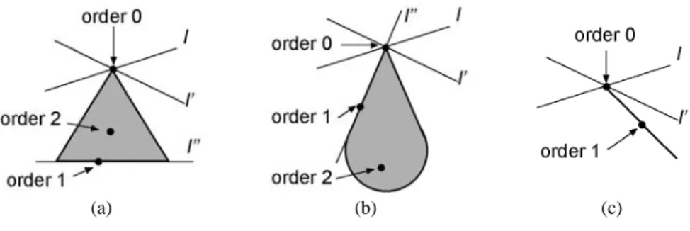
Every point of a closed convex set has an order [24]. Let C be a convex set in d-dimensional Euclidean space Rd. The order of a point x in C, denoted o(x,C), is the dimension of the intersection of all the supporting hyperplanes of C passing through
x. If there is no supporting hyperplane containing x, then x is of order d. One can
prove that the set of points of order d correspond exactly to the points of C’s interior in the sense of Euclidean topology (not equivalent to the interior in point-set topology, as we will see later). For example, suppose a triangle in R². In R², an infinite number of supporting hyperplanes (in this case, lines) can pass through a vertex of the triangle (Fig. 2a). Their intersection is a subspace of dimension 0 (a point corresponding to the given vertex). Thus, this vertex is of order 0. If we take a point being located on the edge of the triangle, there is only one supporting hyperplane. This subspace is of dimension 1 and thus the order of this point is 1 (like all points of the edge other than the two vertices). Lastly, for an interior point of the triangle, there is no supporting hyperplane and thus the order of this interior point is 2 (the dimension of the embedding space). Other examples (a drop-shaped region in R² and a line segment in R²) are presented in Figs. 2b-c.
(a) (b) (c)
Fig. 2. Order of points of various spatial objects in R².
This order concept has been extended from convex sets to topological manifolds with boundary1, such that we can consider a wide variety of spatial objects. The
1 Let n be a positive integer. We denote by Rn+ the subset of tuples (α
1,...,αn) with αn ≥ 0. A subset A of Rd is a topological n-manifold with boundary if each point
definition of the extended concept is beyond the scope of this article; see [21] or [22] for a comprehensive development.
Strictly speaking, the object’s “interior” concept in Euclidean topology, on which the original DM stands, is different from that in point-set topology [25], on which the 9-intersection stands. This difference appears when considering an n-dimensional object embedded in Rd (n < d). In this case, Euclidean topology considers that the object has only a boundary (Fig. 3a), while point-set topology considers that the object consists of a boundary (the set of two endpoints) and an interior (Fig. 3b).
(a) (b)
Fig. 3. Differences between Euclidean topology and point-set topology for n-dimensional
object embedded in Rd (n<d).
To make DM consistent with the models based on point-set topology, the definition of point order has been extended [21], such that the previous definition of order is applied only to the points on the object’s boundary (in the sense of point-set topology), while we consider that the points in object’s interior (in the sense of point-set topology) has the same order with the object’s dimension. In the previous definition of point order, for example, points on a line can be of order 0 or 1 and the points of order 0 are not only line extremities (Fig. 4a). In the extended definition of point order, the line’s “extremities” has order 0 while the line’s “interior” has order 1 (Fig. 4b).
Æ
(a) (b)
Fig. 4. The extension of point order concept for point-set objects.
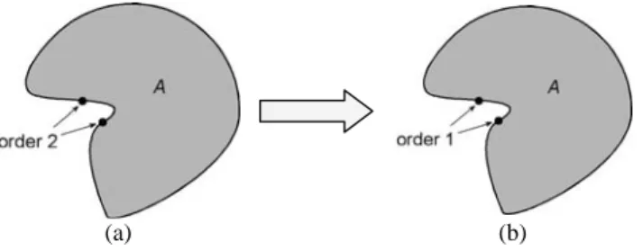
Another issue occurs when applying the previous order definition to the inflexion points. In this case, point’s order is higher than our intuition; i.e. equal to the order of interior points (Fig. 5a). Thus, in the extended definition of point order, if an object of dimension d has a boundary point of order d, the order of this point is reduced to d-1 (Fig. 5b).
(a) (b)
Fig. 5. Modification of inflexion points’ order.
This extended point order concept enables us to consider the segmentation of object’s boundary and consequently to refine binary relationships between objects by considering the connectivity of objects “topological” primitives. It has given birth to the DM model through the concepts of dimensional elements and dimensional relationships.
2.2. Dimensional Elements and Dimensional Relationships
Based on the point order concept, we can consider the subsets of spatial objects, called dimensional elements. Dimensional elements are formally defined as follow: • The n-dimensional element (called nD-element) of a d-dimensional spatial object C
(n ≤ d) corresponds to the set of all of C’s points (or parts) of order 0 to n.
• The nD-element of a spatial object C has an extension and may have a limit. The extension is the subset of C formed by its points of order n, and the limit is the subset of C formed by its points of order 0 to order (n-1).
Thus, if the nD-element has a limit, this limit corresponds to (n-1)D-element. The 0D-element does not have a limit by definition. For instance, let us consider a polygon in Fig. 6a. This polygon is composed by points of order 0, 1, and 2. Thus, we can consider 0D-, 1D-, and 2D-elements for this convex. The different extension and limits are presented in the Figs. 6b-d. It should be noted that each object has one and only one nD-element. Thus, nD-element may be disconnected (e.g., a polygon’s 0D element)
(a) (b) (c) (d)
Fig. 6. (a) Order of points and (b-d) dimensional elements of a polygon
Dimensional relationships between two spatial objects are spatial relationships determined by the connectivity of their dimensional elements. We consider three
connection styles, namely total relation, partial relation and no relation
(non-existent), instead of presence or absence of intersections (Fig. 7).
• A dimensional element is in total relation with another dimensional element if their intersection is equal to the first element, and if the intersection between their extensions is not empty.
• A dimensional element is in partial relation with another dimensional element if their intersection is not equal to the first element, and if the intersection between their extensions is not empty.
• A dimensional element is in no relation (non-existent) with another dimensional element if the intersection between their extensions is empty.
Total relation Partial relation No relation (non-existent)
Fig. 7. Three types of connection styles between two 2D-elements (from black element to grey
element).
2.3. Categorising Spatial Relationships Using Dimensional Relationships
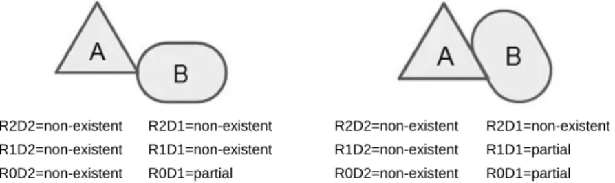
The spatial relationship between two objects can be expressed by the set of connection styles between pairs of dimensional elements of these two objects. For example, let us consider a triangle A (with 2D-, 1D-, and 0D-elements) and an ellipse
B (with 2D- and 1D-elements, but no 0D-element) (Fig. 8). The dimensional
relationships between two objects A and B are determined in the following sequence: first, check the dimensional relationship between A’s 2D-element and each of B’s dimensional elements; then, check the dimensional relationship between A’s 1D-element and each of B’s dimensional 1D-elements, and so on. The dimensional relationships between B and A can be determined by the same approach. A dimensional relationship is coded as RnDm, where R stands for relation, nD for the dimension of the element of the first object, and m for the dimension of the element of the second object. For instance, R2D1 represents the dimensional relationships between the 2D-element of the first object and the 1D-element of the second object.
R2D2=non-existent R2D1=non-existent R2D2=non-existent R2D1=non-existent R1D2=non-existent R1D1=non-existent R1D2=non-existent R1D1=partial R0D2=non-existent R0D1=partial R0D2=non-existent R0D1=partial
3. Reformulating the Dimensional Model with the 9
+-intersection
The Dimensional Model (DM) presented in the previous section has a strong correspondence with the 9-intersection [2]. The 9-intersection and its extensions have been frequently adopted in the studies of topological relations (e.g., [2, 10-13, 15]). Based on point-set topology [25], this model distinguishes the interior, boundary, andexterior of each spatial object, which are also called the object’s topological parts.
The topological relation between two spatial objects A and B is characterized by the intersections of A’s three topological parts and B’s three topological parts, which are concisely represented by the 9-intersection matrix in Eqn. 1.A°, ∂A, and A− are A’s interior, boundary, and exterior, while B°, ∂B, and B− are B’s interior, boundary, and exterior, respectively. Normally, topological relations are distinguished by the presence or absence of these nine types of intersections.
(
)
⎟ ⎟ ⎟ ⎠ ⎞ ⎜ ⎜ ⎜ ⎝ ⎛ ∩ ∂ ∩ ° ∩ ∩ ∂ ∂ ∩ ∂ ° ∩ ∂ ∩ ° ∂ ∩ ° ° ∩ ° = − − − − − − B A B A B A B A B A B A B A B A B A B A M , (1)In DM, as presented in Section 2, the points that form a spatial object are distinguished by their orders. Among the points that form an n-dimensional spatial object, the points of order n form the object’s interior, while the points of order 0 to n-1 form the object’s boundary. This implies the presence of a certain correspondence between DM and the 9-intersection. Meanwhile, if n ≥ 2, DM considers n subsets of the boundary, whereas the 9-intersection cannot distinguish these subsets of the boundary. Instead, the 9+-intersection [15] enables such distinction of boundary
subsets within the framework of the 9-intersection.
The 9+-intersection supports the subdivision of objects’ topological parts by
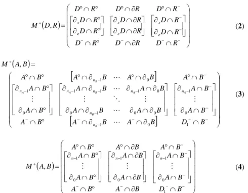
nesting the 9-intersection matrix. For instance, the topological relation between a directed line segment D and a simple region R is captured by the 9+-intersection matrix in Eqn. 2, as D’s boundary consists of two subparts (start point ∂sD and end point ∂eD). The support of such subdivision is useful when a certain topological parts consist of multiple subsets that are qualitatively different. In our case, the boundaries of two spatial objects A and B can be distinguished into multiple subsets, each of which consists of the points of a specific order. Therefore, the relation between two spatial objects A and B is captured by the 9+-intersection matrix in Eqn. 3, where nA is A’s dimension, and nB is B’s dimension, ∂iA is the set of points of order i in A (0 ≤ i ≤ nA–1), and ∂jB is the set of points of order j in B (0 ≤ j ≤ nB–1). Similarly, if we distinguish A’s boundary subset, but not B’s boundary subset, then the relation between A and B is captured by the 9+-intersection in Eqn. 4.
(
)
⎟ ⎟ ⎟ ⎟ ⎟ ⎠ ⎞ ⎜ ⎜ ⎜ ⎜ ⎜ ⎝ ⎛ ∩ ∂ ∩ ° ∩ ⎥ ⎥ ⎦ ⎤ ⎢ ⎢ ⎣ ⎡ ∩ ∂ ∩ ∂ ⎥ ⎦ ⎤ ⎢ ⎣ ⎡ ∂ ∩ ∂ ∂ ∩ ∂ ⎥ ⎦ ⎤ ⎢ ⎣ ⎡ ° ∩ ∂ ° ∩ ∂ ∩ ° ∂ ∩ ° ° ∩ ° = − − − − − − − + R D R D R D R D R D R D R D R D R D R D R D R D R D M e s e s e s , (2)(
)
[
]
[
]
⎟⎟ ⎟ ⎟ ⎟ ⎟ ⎟ ⎠ ⎞ ⎜⎜ ⎜ ⎜ ⎜ ⎜ ⎜ ⎝ ⎛ ∩ ∂ ∩ ∂ ∩ ° ∩ ⎥ ⎥ ⎥ ⎦ ⎤ ⎢ ⎢ ⎢ ⎣ ⎡ ∩ ∂ ∩ ∂ ⎥ ⎥ ⎥ ⎦ ⎤ ⎢ ⎢ ⎢ ⎣ ⎡ ∂ ∩ ∂ ∂ ∩ ∂ ∂ ∩ ∂ ∂ ∩ ∂ ⎥ ⎥ ⎥ ⎦ ⎤ ⎢ ⎢ ⎢ ⎣ ⎡ ° ∩ ∂ ° ∩ ∂ ∩ ° ∂ ∩ ° ∂ ∩ ° ° ∩ ° = − − − − − − − − − − − − − − − − + B D B A B A B A B A B A B A B A B A B A B A B A B A B A B A B A B A M B A B A B A A B n n n n n n n n 1 0 1 0 1 0 0 1 0 0 1 1 1 0 1 0 1 , L M L M O M L M L (3)(
)
⎟ ⎟ ⎟ ⎟ ⎟ ⎟ ⎠ ⎞ ⎜ ⎜ ⎜ ⎜ ⎜ ⎜ ⎝ ⎛ ∩ ∂ ∩ ° ∩ ⎥ ⎥ ⎥ ⎦ ⎤ ⎢ ⎢ ⎢ ⎣ ⎡ ∩ ∂ ∩ ∂ ⎥ ⎥ ⎥ ⎦ ⎤ ⎢ ⎢ ⎢ ⎣ ⎡ ∂ ∩ ∂ ∂ ∩ ∂ ⎥ ⎥ ⎥ ⎦ ⎤ ⎢ ⎢ ⎢ ⎣ ⎡ ° ∩ ∂ ° ∩ ∂ °∩ ° °∩∂ °∩ = − − − − − − − − − − + B D B A B A B A B A B A B A B A B A B A B A B A B A M n n n 1 0 1 0 1 0 1 , M M M (4)Precisely speaking, the captured relations are no longer topological relations when
n ≥ 2, but their refinements, because the order of a point is not invariant under
topological transformation. Therefore, the relations distinguished by the 9+ -intersection matrix in Eqn. 3 or 4 are named binary projective relations. In addition, the model of spatial relations based on the 9+-intersection matrix in Eqn. 3 or 4 is called the projective 9+-intersection. As examples, Fig. 9 shows how the projective
9+-intersection captures projective relations between a triangle and an eclipse. We also call an object whose boundary consists of points of different orders (e.g., polygons) the object with a multi-order boundary, or in short, objects+mob.
⎟ ⎟ ⎟ ⎟ ⎠ ⎞ ⎜ ⎜ ⎜ ⎜ ⎝ ⎛ ¬ ¬ ¬ ⎥ ⎦ ⎤ ⎢ ⎣ ⎡ ¬ ¬ ⎥ ⎦ ⎤ ⎢ ⎣ ⎡ ¬ ⎥ ⎦ ⎤ ⎢ ⎣ ⎡ ¬ φ φ φ φ φ φ φ φ φ φ φ φ ⎟ ⎟ ⎟ ⎟ ⎠ ⎞ ⎜ ⎜ ⎜ ⎜ ⎝ ⎛ ¬ ¬ ¬ ⎥ ⎦ ⎤ ⎢ ⎣ ⎡ ¬ ¬ ⎥ ⎦ ⎤ ⎢ ⎣ ⎡ ¬ ¬ ⎥ ⎦ ⎤ ⎢ ⎣ ⎡ ¬ φ φ φ φ φ φ φ φ φ φ φ φ
The projective 9+-intersection is upward compatible with DM, because, given a 9+ -intersection matrix in Eqn. 3, we can uniquely determine the dimensional relation in DM (i.e., a complete set of RnDm expressions) through the conversion formula in Eqn. 5 (compare Figs. 8-9). Meanwhile, the new model and DM has the following differences:
• DM considers the intersections with respect to k-dimensional element (i.e., the set of points of order 1 to k), while the new model considers the intersections with respect to the extension of k-dimensional element (i.e., the set of points of order k). • The new model also considers the intersections with respect to the objects’
exteriors.
• DM distinguishes three styles of intersections (i.e., partial, total, and non-existent), while the new model distinguishes only two styles (i.e., X intersects with Y or not). This change does not reduce the model’s representation capability, because it becomes possible to determine whether X overlaps with Y (partial relation), X is included in Y (total relation), or else (no relation), considering the intersections concerning the objects’ exteriors.
( )
(
( )
)
( )(
( )
)
( ) ( ) existent non m n B A total m n B B A B A partial m n B B A B A B O i B B B B A O i A A A A m n k B O n k n m n k B O n k n m n i i B O i i A O -D R D R D R 1 0 , 1 0 , 1 1 = → = ∩ = → = ⎟ ⎠ ⎞ ⎜ ⎝ ⎛ ∪ ∪ ∩ ∧ ≠ ∩ = → ≠ ⎟ ⎠ ⎞ ⎜ ⎝ ⎛ ∪ ∪ ∩ ∧ ≠ ∩ − < ≤ ∂ = ° = − < ≤ ∂ = ° = − + = − + = φ φ φ φ φ (5)The projective 9+-intersection serves as a refinement of the 9-intersection, as easily expected from the shape of the underlying matrix. This means that spatial relations under the new model can be systematically categorized based on the sets of topological relations identified in the previous studies (e.g., [2]), as well as that the spatial arrangement of two objects that falls into the same topological relations in the previous relation set may be distinguished by the new model. The next sections discuss such characteristics of the new model as a refinement of the 9-intersection.
4.
Projective Relations between a Region with Multi-Order
Boundary and a Region
There are in theory 24×3 = 4096 projective relations between a region with multi-order boundary and a region in R2, because the relations are represented by the 9+ -intersection matrix with 4×3 two-valued elements (e.g., Fig. 9). However, only a small subset of these relations can be realized in a particular space. As a refinement of the 9-intersection, all the constraints of the 9-intersection for topological region-region relations, identified in [2], can be applied to the projective 9+-intersection. In addition, due to the subdivision of the region’s boundary, the following seven specific
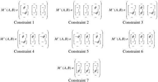
constraints are additionally applied, where the set of points of order n in the boundary of a spatial object X is called X’s order n boundary:
• Constraint 1: If A’s order 0 boundary intersects with B’s interior, then A’s order 1 boundary must intersect with B’s interior
• Constraint 2: If A’s order 0 boundary intersects with B’s exterior, then A’s order 1 boundary must intersect with B’s exterior
• Constraint 3: If A’s order 0 boundary intersects with B’s interior and B’s exterior, then A’s boundary must intersect with B’s boundary
• Constraint 4: If A’s order 1 boundary intersects only with B’s exterior, then A’s order 0 boundary must not intersect with B’s interior
• Constraint 5: If A’s order 1 boundary intersects only with B’s interior, then A’s order 0 boundary must not intersect with B’s exterior
• Constraint 6: A’s order 1 boundary intersects with at least one part of B • Constraint 7: A’s order 0 boundary intersects with at least one part of B Fig. 10 illustrates these constraints using the 9+-intersection matrix.
⎟ ⎟ ⎟ ⎟ ⎠ ⎞ ⎜ ⎜ ⎜ ⎜ ⎝ ⎛ − − − ⎥ ⎦ ⎤ ⎢ ⎣ ⎡ − − ⎥ ⎦ ⎤ ⎢ ⎣ ⎡ − − ⎥ ⎦ ⎤ ⎢ ⎣ ⎡ ¬ − − − ≠ + φ φ ) , (AB M ⎟ ⎟ ⎟ ⎟ ⎠ ⎞ ⎜ ⎜ ⎜ ⎜ ⎝ ⎛ − − − ⎥ ⎦ ⎤ ⎢ ⎣ ⎡ ¬ ⎥ ⎦ ⎤ ⎢ ⎣ ⎡ − − ⎥ ⎦ ⎤ ⎢ ⎣ ⎡ − − − − − ≠ + φ φ ) , (AB M ⎟ ⎟ ⎟ ⎟ ⎠ ⎞ ⎜ ⎜ ⎜ ⎜ ⎝ ⎛ − − − ⎥ ⎦ ⎤ ⎢ ⎣ ⎡ ¬ − ⎥ ⎦ ⎤ ⎢ ⎣ ⎡ ⎥ ⎦ ⎤ ⎢ ⎣ ⎡ ¬ − − − − ≠ + φ φ φ φ ) , (AB M
Constraint 1 Constraint 2 Constraint 3
⎟ ⎟ ⎟ ⎟ ⎠ ⎞ ⎜ ⎜ ⎜ ⎜ ⎝ ⎛ − − − ⎥ ⎦ ⎤ ⎢ ⎣ ⎡ − ¬ ⎥ ⎦ ⎤ ⎢ ⎣ ⎡ − ⎥ ⎦ ⎤ ⎢ ⎣ ⎡ ¬ − − − ≠ + φ φ φ φ ) , (AB M ⎟ ⎟ ⎟ ⎟ ⎠ ⎞ ⎜ ⎜ ⎜ ⎜ ⎝ ⎛ − − − ⎥ ⎦ ⎤ ⎢ ⎣ ⎡ ¬ ⎥ ⎦ ⎤ ⎢ ⎣ ⎡ − ⎥ ⎦ ⎤ ⎢ ⎣ ⎡ − ¬− − − ≠ + φ φ φ φ ) , (AB M ⎟ ⎟ ⎟ ⎟ ⎠ ⎞ ⎜ ⎜ ⎜ ⎜ ⎝ ⎛ − − − ⎥ ⎦ ⎤ ⎢ ⎣ ⎡ − ⎥ ⎦ ⎤ ⎢ ⎣ ⎡ − ⎥ ⎦ ⎤ ⎢ ⎣ ⎡ − − − − ≠ + φ φ φ ) , (AB M
Constraint 4 Constraint 5 Constraint 6
⎟ ⎟ ⎟ ⎟ ⎠ ⎞ ⎜ ⎜ ⎜ ⎜ ⎝ ⎛ − − − ⎥ ⎦ ⎤ ⎢ ⎣ ⎡− ⎥ ⎦ ⎤ ⎢ ⎣ ⎡− ⎥ ⎦ ⎤ ⎢ ⎣ ⎡−− − − ≠ + φ φ φ ) , (AB M Constraint 7
Fig. 10. New constraints applied to the matrix of the projective 9+-intersection.
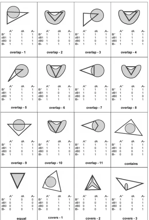
By applying these constraints, the number of relations is reduced from 4096 to 30 (Figs. 11-12). All of these 30 relations normally have geometric realization in R2. Exceptionally, when A’s order 0 boundary consist of three distinctive subparts (i.e., when A is a triangle), the relation “overlap-11” is impossible. These 30 relationships are indeed a refinement of eight topological relations between regions. Consequently, we have decided to keep the same names (i.e. overlap, contains, inside, covers,
coveredBy, equal, meet, and disjoint [4]) and just added a number to them which
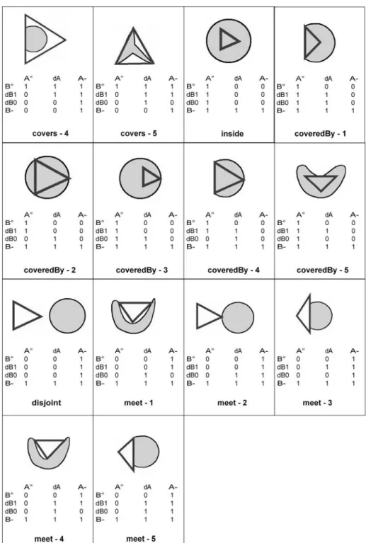
Fig. 11. Thirty possible projective relations between a region with a multi-order boundary and a
Fig. 12. Thirty possible projective relations between a region with a multi-order boundary and a
5. Conceptual Neighbourhood Graph
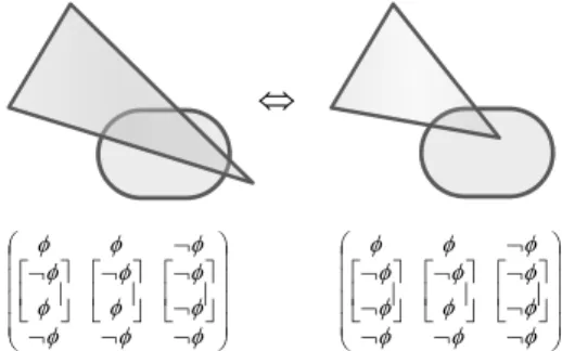
The 30 projective relations derived in the previous section are organized into a similarity-based schema, called a conceptual neighbourhood graph [26]. Conceptual neighbourhood graphs are frequently used for schematizing, analyzing, and visualizing a set of spatial relations [4, 9, 11, 14, 15, 19, 26-30]. In a conceptual neighbourhood graph, each node corresponds to a spatial relation, and two nodes are linked if their corresponding relations are conceptual neighbours. Different definitions of conceptual neighbours lead to different graph shapes for the same set of relations [26, 28]. This paper considers that two projective relations between a region with a multi-order boundary (region+mob) A and a region B are conceptual neighbours if there is a configuration of one relation that can switch to a configuration of another relation by transforming A continuously, such that one vertex or edge loses/gains one intersection with B’s interior, boundary, or exterior. Accordingly, the transformation in Fig. 13a establishes continuous neighbours, but that in Fig. 13b, which yields the generation of three intersections (∂0A∩B°, ∂1A∩B°, and ∂1A∩∂B) and loss of
one intersection (∂0A∩∂B), is not accepted. Acceptable continuous transformation
always results in the change of one of six elements in the middle two rows of the matrix (i.e., ∂0A∩B°, ∂0A∩∂B, ∂0A∩B−, ∂1A∩B°, ∂1A∩∂B, and
−
∩ ∂1A B ).
Thus, all candidates for conceptual neighbours are derived computationally from the patterns of the 9+-intersection matrix that correspond to the 30 projective relations.
⇔ ⎟ ⎟ ⎟ ⎟ ⎠ ⎞ ⎜ ⎜ ⎜ ⎜ ⎝ ⎛ ¬ ¬ ¬ ⎥ ⎦ ⎤ ⎢ ⎣ ⎡ ¬ ¬ ⎥ ⎦ ⎤ ⎢ ⎣ ⎡ ¬ ⎥ ⎦ ⎤ ⎢ ⎣ ⎡ ¬ φ φ φ φ φ φ φ φ φ φ φ φ ⎟ ⎟ ⎟ ⎟ ⎠ ⎞ ⎜ ⎜ ⎜ ⎜ ⎝ ⎛ ¬ ¬ ¬ ⎥ ⎦ ⎤ ⎢ ⎣ ⎡ ¬ ¬ ⎥ ⎦ ⎤ ⎢ ⎣ ⎡ ¬ ¬ ⎥ ⎦ ⎤ ⎢ ⎣ ⎡ ¬ φ φ φ φ φ φ φ φ φ φ φ φ ⎟ ⎟ ⎟ ⎟ ⎠ ⎞ ⎜ ⎜ ⎜ ⎜ ⎝ ⎛ ¬ ¬ ¬ ⎥ ⎦ ⎤ ⎢ ⎣ ⎡ ¬ ¬ ⎥ ⎦ ⎤ ⎢ ⎣ ⎡ ¬ ⎥ ⎦ ⎤ ⎢ ⎣ ⎡ ¬ φ φ φ φ φ φ φ φ φφ φ φ ⇔ ⎟ ⎟ ⎟ ⎟ ⎠ ⎞ ⎜ ⎜ ⎜ ⎜ ⎝ ⎛ ¬ ¬ ¬ ⎥ ⎦ ⎤ ⎢ ⎣ ⎡ ¬ ¬ ⎥ ⎦ ⎤ ⎢ ⎣ ⎡¬ ⎥ ⎦ ⎤ ⎢ ⎣ ⎡ ¬ ¬ ¬ φ φ φ φ φ φ φ φ φ φ φ φ (a) (b)
Fig. 13. (a) A continuous transformation that establishes conceptual neighbours and (b) another
continuous transformation that does not establish conceptual neighbours.
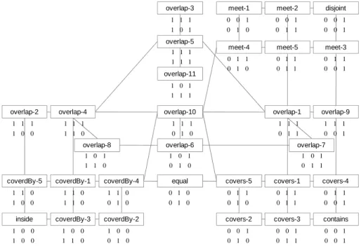
Based on the previous definition of conceptual neighbours, we developed the conceptual neighbourhood graph of the 30 projective region+mob-region relations (Fig. 14). Basically, the developed graph has both horizontal and vertical symmetry axes, even though the upper-left part is missing and overlap-refinements do not follow the horizontal symmetric axis. The spatial arrangement of the 30 projective region+mob-region relations in this conceptual neighbourhood graph corresponds to the arrangement of topological region-region relations in their conceptual neighbourhood graph [4] (Fig. 15a). This highlights the characteristics of these 30 projective region+mob-region relations as the refinement of topological region-region relations. The comparison of two graphs shows that the number of steps from one relation to
another relation is larger in our graph, except those from disjoint to contains and vice versa (Fig. 15b). overlap-3 overlap-7 overlap-8 disjoint meet-3 meet-2 meet-5 meet-1 meet-4 contains covers-4 covers-3 covers-1 covers-2 inside coverdBy-5 coverdBy-3 coverdBy-1 coverdBy-2 overlap-9 overlap-2 equal overlap-6 coverdBy-4 covers-5
overlap-4 overlap-10 overlap-1
overlap-5 1 0 0 1 1 1 1 0 0 1 1 0 1 1 0 1 1 0 0 1 0 1 1 0 0 1 1 1 0 1 0 0 1 1 1 1 0 1 0 0 1 0 1 0 1 1 1 1 1 1 1 1 1 1 1 0 0 1 1 0 1 1 0 1 1 0 0 1 0 1 1 0 0 1 0 0 0 1 0 1 1 0 0 1 0 0 1 0 0 1 1 1 0 1 0 1 overlap-11 1 1 1 1 0 1 0 1 0 1 1 1 0 1 0 1 0 1 1 0 0 1 0 0 1 1 0 1 0 0 0 1 0 1 0 0 1 0 0 1 0 0 1 1 0 1 0 0 0 1 0 1 0 0 0 1 0 0 1 1 0 1 1 0 1 1 0 0 1 0 1 1 0 1 1 1 1 1 1 1 0 1 1 1
Fig. 14. Conceptual neighbourhood graphs of the 30 projective relations between a region with
a multi-order boundary and a region in R², together with the six elements in the matrix’s middle two rows. disjoint meet overlap coveredBy inside covers equal contains disjoint meet overlap coveredBy inside cover equal contain 4 s te p s 4 steps 4 steps (a) (b)
Fig. 15. (a) Conceptual neighbourhood graphs of eight topological region-region relations [4]
and (b) numbers of steps between nodes in the corresponding conceptual neighbourhood graph of projective region+mob-region relations in Fig. 14.
Through the analysis of the developed conceptual neighbourhood graph, we found the following facts:
• The pairs of relations with one difference in the matrices’ middle two rows, where one has
(
¬φ φ ¬φ)
and another has(
φ φ ¬φ)
or(
¬φ φ φ)
with respect to one of these two rows (e.g., overlap-3 and overlap-9), are not conceptual neighbours, because the shift between these two relations require that one vertex or one edge of the triangle skips over the region’s boundary (Fig. 16).• The matrices’ middle two rows of the relations on the graph’s vertical centre line (i.e., overlap-3, -5, -6, -10, -11, and equal) are left-right symmetric.
• In each pair of relations located symmetrically with respect to the graph’s vertical centre line (e.g., inside and contain), the matrix of one relation is derived from the matrix of another relation by exchanging the matrix’s elements with respect to
°
B and B−. This means that one relation is derived from another relation by reversing B’s interior and exterior, assuming a spherical surface that embeds the configurations of the relations.
• Similarly, in each pair of relations located symmetrically with respect to the graph’s horizontal centre line (e.g., disjoint and contain), the matrix of one relation is derived from the matrix of another relation by exchanging the matrix’s elements with respect to A° and A−. This means that one relation is derived from another relation by reversing A’s interior and exterior, assuming a spherical surface that embeds the configurations of the relations.
• Overlap-1 to overlap-11 follow the vertical symmetric axis only. We can consider a virtual graph that is horizontally and vertically symmetric (Fig. 17), considering the patterns of their projective 9+-intersection matrices. In this graph, however, overlap-1' to overlap-10' have no geometric realization.
From the third and fourth findings, we can expect that the upper-left empty part of the conceptual neighbourhood graph in Fig. 14 potentially domiciles the relations that appear in a spherical surface, but not in a plane. This is analogous to Egenhofer’s [11] finding of three additional region-region relations on a spherical surface, namely
attaches, embraces, and entwined. Thus, it is expected that the relations at the graph’s
upper-left empty part neighbour should be the refinements of attaches, embraces, and entwined relations. ⎟ ⎟ ⎟ ⎟ ⎠ ⎞ ⎜ ⎜ ⎜ ⎜ ⎝ ⎛ ¬ ¬ ¬ ⎥ ⎦ ⎤ ⎢ ⎣ ⎡ ¬ ¬ ⎥ ⎦ ⎤ ⎢ ⎣ ⎡¬ ⎥ ⎦ ⎤ ⎢ ⎣ ⎡ ¬ ¬ ¬ φ φ φ φ φ φ φ φ φ φ φ φ ⇔ ⎟ ⎟ ⎟ ⎟ ⎠ ⎞ ⎜ ⎜ ⎜ ⎜ ⎝ ⎛ ¬ ¬ ¬ ⎥ ⎦ ⎤ ⎢ ⎣ ⎡ ¬ ¬ ⎥ ⎦ ⎤ ⎢ ⎣ ⎡¬ ⎥ ⎦ ⎤ ⎢ ⎣ ⎡¬ ¬ φ φ φ φ φ φ φ φ φ φ φ φ
Fig. 16. Non-continuous transformation, even though that yields only one change in the middle
overlap-3 overlap-7 overlap-8 overlap-9 overlap-2 overlap-6
overlap-4 overlap-10 overlap-1
overlap-5 1 0 0 1 1 1 0 1 1 1 0 1 0 0 1 1 1 1 1 0 1 1 1 1 1 1 1 1 1 1 1 1 0 1 0 1 overlap-11 1 1 1 1 0 1 0 1 0 1 1 1 0 1 0 1 0 1 0 1 1 1 1 1 1 1 0 1 1 1 overlap-7' overlap-8' overlap-9' overlap-2' overlap-6'
overlap-4' overlap-10' overlap-1'
1 0 0 1 1 1 0 1 1 1 0 1 0 0 1 1 1 1 1 1 0 1 0 1 0 1 0 1 1 1 0 1 0 1 0 1 0 1 1 1 1 1 1 1 0 1 1 1
Fig. 17. Virtual symmetry of the conceptual neighbourhood graph in Fig. 3 with respect to
overlap refinements. Overlap-1' to overlap-10' have no geometric realization, however.
6. Conclusions
This paper developed a new model of projective relations based on the Dimensional Model [22] and the 9+-intersection [15]. As a first step, this paper identified 30 projective relations between a region with a multi-order boundary and a region (i.e., projective region+mob-region relations) in R2, and schematized these 30 relations into a conceptual neighbourhood graph. Naturally, the next target is the relations between two regions, both with a multi-order boundary (i.e., projective region+mob- region+mob relations). By replacing regions by regions with multi-order boundaries, the number of projective relations will increase, and the conceptual neighbourhood graph will become more complicated (probably more high-dimensional). It is also expected that the shapes of regions with multi-order boundaries influence the realizability of some projective relations. For instance, a triangle and a quadrilateral cannot have an equal relation.
Another challenge is to identify and analyze projective relations in a three dimensional space. Systematic analyses of three-dimensional topological relations were conducted in [10, 21], identifying many relations that cannot be realized in R2. Similar analysis should be possible for projective relations.
An interesting and promising topic is the composition of projective relations. The composition of spatial relations is an operation that derives possible relations between two spatial objects from the knowledge of the relations between each of these objects
and the common third object. Such compositions of spatial relations have been frequently discussed as a foundation of qualitative spatial reasoning [6, 11, 14, 18, 27-29, 31, 32]. It is an interesting question whether the compositions of projective relations become crisper than those of topological relations, as the projective relations consider the dimensional characteristics of the regions’ boundaries.
References
1. Egenhofer, M., Franzosa, R.: Point-Set Topological Spatial Relations. International Journal of Geographical Information Systems 5, 161-174 (1991)
2. Egenhofer, M., Herring, J.: Categorizing Binary Topological Relationships between Regions, Lines and Points in Geographic Databases. In: Egenhofer, M., Herring, J., Smith, T., Park, K. (eds.): NCGIA Technical Reports 91-7. National Center for Geographic Information and Analysis, Santa Barbara, CA, USA (1991)
3. Randell, D., Cui, Z., Cohn, A.: A Spatial Logic Based on Regions and Connection. In: Nebel, B., Rich, C., Swarout, W. (eds.): 3rd International Conference on Knowledge Representation and Reasoning, pp. 165-176. Morgan Kaufmann (1992)
4. Egenhofer, M., Al-Taha, K.: Reasoning about Gradual Changes of Topological Relationships. In: Frank, A., Campari, I., Formentini, U. (eds.): Theories and methods of spatio-temporal reasoning in geographic space, LNCS, vol. 639, pp. 196-219. Springer (1992)
5. Clementini, E., Di Felice, P., van Oosterom, P.: A Small Set of Formal Topological Relationships Suitable for End-User Interaction. In: Abel, D., Ooi, B.C. (eds.): 3rd International Symposium on Advances in Spatial Databases, LNCS, vol. 692, pp. 277-295. Springer (1993)
6. Egenhofer, M.: Deriving the Composition of Binary Topological Relations. Journal of Visual Languages and Computing 5, 133-149 (1994)
7. Egenhofer, M., Franzosa, R.: On the Equivalence of Topological Relations International Journal of Geographical Information Systems 9, 133-152 (1995)
8. Clementini, E., Di Felice, P.: Topological Invariants for Lines. IEEE Transactions on Knowledge and Data Engineering 10, 38-54 (1998)
9. Hornsby, K., Egenhofer, M., Hayes, P.: Modeling Cyclic Change. In: Chen, P., Embley, D., Kouloumdjian, J., Liddle, S., Roddick, J. (eds.): Advances in Conceptual Modeling, LNCS, vol. 1227, pp. 98-109. Springer (1999)
10. Zlatanova, S.: On 3D Topological Relationships. In: 11th International Workshop on Database and Expert Systems Applications, pp. 913-924. IEEE Computer Society (2000) 11. Egenhofer, M.: Spherical Topological Relations. Journal on Data Semantics III, 25-49
(2005)
12. Schneider, M., Behr, T.: Topological Relationships between Complex Spatial Objects. ACM Transactions on Database Systems 31, 39-81 (2006)
13. Nedas, K., Egenhofer, M., Wilmsen, D.: Metric Details of Topological Line-Line Relations. International Journal of Geographical Information Science 21, 21-48 (2007)
14. Kurata, Y., Egenhofer, M.: The Head-Body-Tail Intersection for Spatial Relations between Directed Line Segments. In: Raubal, M., Miller, H., Frank, A., Goodchild, M. (eds.): GIScience'06, LNCS, vol. 4197, pp. 269-286. Springer (2006)
15. Kurata, Y., Egenhofer, M.: The 9+-Intersection for Topological Relations between a Directed Line Segment and a Region. In: Gottfried, B. (ed.): 1st International Symposium for Behavioral Monitoring and Interpretation, pp. 62-76 (2007)
17. Frank, A.: Qualitative Spatial Reasoning about Distances and Directions in Geographic Space. Journal of Visual Languages and Computing 3, 343-371 (1992)
18. Freksa, C.: Using Orientation Information for Qualitative Spatial Reasoning. In: Frank, A., Campari, I., Formentini, U. (eds.): International Conference GIS - From Space to Territory: Theories and Methods of Spatio-Temporal Reasoning in Geographic Space, LNCS, vol. 639, pp. 162-178. Springer (1992)
19. Schlieder, C.: Reasoning about Ordering. In: Frank, A., Kuhn, W. (eds.): COSIT '95, LNCS, vol. 988, pp. 341-349. Springer (1995)
20. Clementini, E., Billen, R.: Modeling and Computing Ternary Projective Relations between Regions. IEEE Transactions on Knowledge and Data Engineering 18, 799-814 (2006) 21. Billen, R.: Nouvelle Perception De La Spatialité Des Objets Et De Leurs Relations.
Développment D'une Modélisation Tridimensionnelle De L'information Spatiale. Department of Geography, Ph.D. Thesis. University of Liège, Liège, Belgium (2002)
22. Billen, R., Zlatanova, S., Mathonet, P., Boniver, F.: The Dimensional Model: A Framework to Distinguish Spatial Relationships. In: Richardson, D., van Oosterom, P. (eds.): Advances in spatial data handling: 10th International Symposium on Spatial Data Handling, pp. 285-298. Springer (2002)
23. Billen, R., Clementini, E.: Etude Des Caractéristiques Projectives Des Objets Spatiaux Et De Leurs Relations. Revue Internationale de Géomatique 14, 145-165 (2004)
24. Berger, M.: Géométrie 3 : Convexes Et Polytopes, Polyèdres Réguliers, Aires Et Volumes. Cedic/Fernand Nathan, Paris (1978)
25. Alexandroff, P.: Elementary Concepts of Topology. Dover Publications, Mineola, NY (1961)
26. Freksa, C.: Temporal Reasoning Based on Semi-Intervals. Artificial Intelligence 54, 199-227 (1992)
27. Galton, A.: Lines of Sight. In: AI and Cognitive Science '94, pp. 103-113. Dublin University Press (1994)
28. Egenhofer, M., Mark, D.: Modeling Conceptual Neighborhoods of Topological Line-Region Relations. International Journal of Geographical Information Systems 9, 555-565 (1995) 29. Gottfried, B.: Reasoning about Intervals in Two Dimensions. In: Thissenm, W., Pantic, M.,
Ludema, M. (eds.): IEEE International Conference on Systems, Man and Cybernetics, pp. 5324-5332 (2004)
30. Van de Weghe, N., De Maeyer, P.: Conceptual Neighbourhood Diagrams for Representing Moving Objects. In: 2nd International Workshop on Conceptual Modeling for Geographic Information Systems, LNCS, vol. 3770, pp. 228-238. Springer (2005)
31. Moratz, R., Renz, J., Wolter, D.: Qualitative Spatial Reasoning about Line Segments. In: Horn, W. (ed.): 14th European Conference on Artificial Intelligence, pp. 234-238. IOS Press (2000)
32. Van de Weghe, N., Kuijpers, B., Bogaert, P., De Maeyer, P.: A Qualitative Trajectory Calculus and the Composition of Its Relations. In: Rodriguez, A., Cruz, I., Egenhofer, M., Levashkin, S. (eds.): The 1st International. Conference on Geospatial Semantics, LNCS, vol. 3799, pp. 60-76. Springer (2005)