Decision Support for Improving Public Transport Network

Texte intégral

(1)DECISION SUPPORT FOR IMPROVING PUBLIC TRANSPORT NETWORK VANRAES Niko – CORNÉLIS Bernard – DONNAY Jean-Paul Abstract On the question of accessibility in a public transport network, isochronous maps are the common rule. Those maps are based on shortest distance algorithms run over simple or simplified networks. This contribution aims at representing the actual spatial distribution of the public transport offer in order to improve the usefulness to the urban community and to predict the evolution of the network according to the expected development of the agglomeration. The study combines the street (walking distance) and public transportation (buses) networks. The analyses rely on time-tables and road maps completed by the public transportation company (TEC). Moreover, it makes use of built-up areas derived from satellite imagery. The processing requires raster- as well as vector-based procedures which have been achieved notably with the IDRISI software. Nevertheless the implementation of the decision rule relies on an original routine written by the authors. The area of interest concerns a part of the agglomeration of Liège (Belgium), including two secondary poles, highlighting their relation with the centre of the city and with each other. First the paper presents the typology of the public transport routes. Then the methodology elaborated for each transportation type is analysed; the shortest distance routes and their alternatives are extracted and combined within a raster process. The obtained results and their operationality are finally presented and the paper concludes with possible improvements of the methodology.. 1. INTRODUCTION For a few years public transportation is a question that has been much debated in urban management. The increasing motor car traffic and its pressure on urban life have led urban decision-makers to pay attention to alternative solutions where public transport is inescapable (MET, 1996). Before improving the offer in public transport, it must be studied in its actual form in order to highlight its forces and weaknesses. This paper attempts to set out the real spatial distribution of the public transport offer. This offer is expressed as the time required to go from any point within the area of interest to a final destination (or from one selected origin to all the other locations in the area). Travelling implies a cost (CANCALON and GARGAILLO, 1991 ; ROY, 1991) which is a function of the travelling time. Therefore shortest time-cost route should have to be chosen according to the decision rule. The search for the shortest time-cost route is justified by the travellers’ wish to minimise their travelling cost. Such routes can be found with different algorithms such as the Dijkstra’s algorithm (DIJKSTRA, 1959, in CANCALON and GARGAILLO, 1991; DONNAY, 1983a, 1983b;. 1.

(2) ENGELEN and BRANS, 1980; ROY, 1991). However, the full trips are not necessary made via these routes due to the nature of the public transport itself. In order to find the spatial distribution of the public transport offer, isochronous maps are often made (DUSSART, 1939 et 1959; AUGUSTE, 1977; BAUDOT et LALOUX, 1980; VANCRAEYNEST, 1986; KUMMERT et VANDERMOTTEN, 1975). The length of the route takes in account the waiting time, connection time, etc. To make an isochronous map it is necessary to find the shortest time-cost route. This is a central point of the problem because many authors consider only the fastest line. Sometimes the features of many lines are aggregated. Speed is supposed to be identical for all the lines even though this is not always the case (id.). Another problem is the extension of the walking time beyond the stops : should the distance be considered along the roads or in a straight line ? Moreover, classic isochronous maps take a long time to draw up. Furthermore, each new point necessitates the realisation of a new map (KUMMERT et VANDERMOTTEN, 1975). On the other side, such maps are almost calculated over the whole day. This contribution defines first the features of public transport networks and establishes a typology of public transport routes. Afterwards, the methodology used for the two parts public transport journey is developed. Finally, results obtained on a concrete case are discussed and possible improvements are presented. 2. PUBLIC TRANSPORTATION NETWORKS 2.1. Distinctive features of public transport networks A trip done with a private transport mode is almost realised with one vehicle. Besides the walking at the beginning and at the end of a public transport trip, connections are often necessary to reach the destination when using public transport. There can also be different services on the same link. For instance an express bus and a regular bus. Travelling by public transport is not possible at any time (ROY, 1991). The travellers have to wait for the passage of the vehicles at the stop. The fastest line is thus not always available. Consequently, a public transport network is very different from networks such as the road network. 2.2. Typology of the public transport routes When one think of a public transportation network he often thinks of a simple network such as can be seen on the subway maps of Paris or London. However, public transportation networks are frequently more complex. The complexity generally increases when the vehicles are not attached to tracks.. 2.

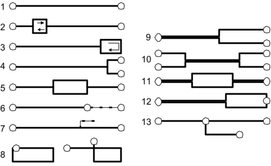
(3) If in dense city centres the routes remain simple this is not always the case in the suburbs. Those areas are characterised with greater people dispersion and thus imply a more complex network. As a consequence buses mostly serve such areas since they have more freedom in their routes. Diverse public transport networks have been analysed through the maps delivered by transport companies to their users. A typology of the different configurations of the public transport routes has been realised [Figure 1] (Vanraes, 1997). This typology demonstrates the complexity of public transport networks. Figure 1. Typology of public transport routes (1 to 8) and combination of public transport routes (9 to 13).. 1 2 9 3 4 5 6 7. 10 11 12 13. 8 Different routes of one bus linei: 1. Simple route – 2. Difference between the outward route and return route – 3. Terminal loop – 4. Variant at the terminus – 5. Variant in a part of the route – 6. Extension – 7. Lateral Extension – 8 Circular route. Combination of routes of two bus lines: 9. Different destinations – 10 Different origin and destination – 11. Different part of the route – 12. Different part at the end of the routes – 13. “Rabattement” Line.. 2.3. Studied network The method was applied to a part of Liège, third urban area in Belgium with its 600.000 inhabitants. The studied area is triangular shaped. The top of this triangle is in the centre and the triangle stretches to the rural outskirts. Two sides of the area of interest are limited by motorways. Motorways are an obstacle for pedestrians since they can only be crossed at limited places. The network covering this area is made out of twenty-one bus lines. Two major bus roads link the centre and two secondary poles of the urban area: Ans and. 3.

(4) Rocourt. High frequency lines follow those roads. The two poles are only linked with two low frequency lines (one vehicle per hour). 3. PUBLIC TRANSPORT TRIP A public transport trip can be split in different parts: -. the walking trip to the public transport vehicle stop (bus stop, station) will be detailed further; the waiting for the passage of the vehicle; the journey in the vehicle from the origin stop to the destination stop; eventually a connection will be necessary to gain the destination.. 3.1. The waiting time The waiting time, the journey and an eventual connection are specific to the public transport network itself. Passage frequency, , at a stop is the quantity of vehicles passing at a stop in a given interval and period, T , is the time passing between two halts of a vehicle at a stop, the mean waiting time for a traveller, , will TIME 1. ALLOCATE >0 Global route time of the nearest node. NODES. >0 = Global Route time for the node 0 = other pixels. TOT.TIME 1. +. COST 1. FOOT 1. Total time for the road pixels. >0 Time necessary. ROADS. FRICTION 1. >0 = distance in to reach the x2.52 nearsest node (only pixels to the for roads pixels) nearest node. TOT.TIME 2. 1 = road pixels RECLASS 1 = road pixels 0 = other pixles -1 = other pixles. + Total time. ALLOCATE. FRICTION 2. All pixels = 1. COST 2. COSTGROW. FOOT 2. Pixels = distance Pixels = time to to the nearest x2.52 reach the nearest road pixel road pixel. TIME 2. >0 Total time of the nearest road pixel. be: w  T / 2 with T  [time interval]/. If the time interval is equal to one hour the mean waiting time will be: w  30 /  . The period used is a mean period, which means the time between two passages of a vehicle at a given stop is considered to be constant ( T  Ti ). If this is true for important bus routes which are regularly cadenced, it is not the case with less important lines. However the mean period is often accepted as a good approximation but the network analyst must know that the precision will decrease with the irregularity of the periods especially when they are important. In fact, even for important bus routes, the period does not remain constant the whole day. Different phases can be observed: peak phases, peak-off phases, evening phase, and so on (ORFEUIL J.-P. and TROULAY P., 1989 ). The mean period measured over a whole day will not reflect the reality. For instance, some lines have a short period in peak hours and a long period during the rest of the day (such as peak lines). A serious study should thus only be done over a precise phase. 3.2. The journey in the vehicle The journey in the vehicle from the origin stop to the destination stop is available in the time schedules of public transport companies. Such timetables are not often complete in the sense that the information is not available for all the stops of a. 4.

(5) bus line. In this case the passage time can be found with the distance separating two stops where the time is known. 3.3. Connections When travelling by public transport one or more connections are often necessary to join the destination stop. As a consequence, the travellers will be submitted to the frequency of the other lines. It is also estimated that at least two minutes are necessary to a make a connection (KUMMERT and VANDERMOTTEN, 1975) : if the second vehicle arrives at the same time as the first one at the connection stop, it will be difficult for the users to make the connection because, for instance, the road must be crossed, the platforms are not on the same level, etc… So far, the global time for a journey from a starting stop to a destination stop can be expressed as: c. time  2c   ( 1. 30. .  Ri ). With: c: the number of connections; : the frequency R: the time passed in the vehicle from the origin stop to the destination stop. 3.4. Multiple services. The difficulty of a public transportation network is that is often more than one line joins two stops. Those lines can have different routes, number of stops, frequencies, route times. To solve that problem, the contribution of each line joining the stops and respecting specific condition was taken into account. The mean waiting time for a vehicle is 30 /  i and the mean route time is a weighted mean.  i Ri i. . i. . But those multiple service formulas can not be applied in. i. i. each case. The question, for instance, is “if a line takes thirty minutes to join the destination stop and an other line takes forty-five minutes to reach the same stop, will the traveller take indifferently the first vehicle passing at the stop independently of the line or will he chose a specific line regarding the route time?”. This question can be expressed as: ”if the traveller misses the vehicle of the first line that takes thirty minutes to join his destination will he take the second line that takes forty-five minutes but passes at the stop before the next bus of the first line?”. The answer is. 5.

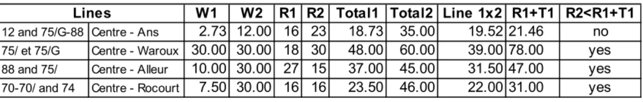
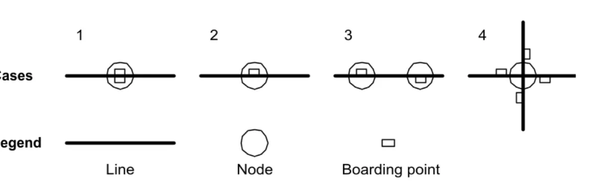
(6) considered positive if the vehicle of the second line arrives at the destination stop before the next vehicle of the first line”. The decision rule will thus be “the multiple service can be calculated if R2 R1+W1” [Table 1]. This decision rule amounts to the same thing as saying the traveller tolerates a greater difference in the route times if the frequency of the connections between his origin and destination stop are weak. This way of acting is logical if we remark that most public transport users don’t know the exact passage time of the vehicles but have an idea of the frequency and the time necessary to reach their destination stop. They chose their line(s) with these parameters Table 1. Multiple service examples in the studied network (units: decimal minutes). W1 2.73 Centre - Waroux 30.00 10.00 Centre - Alleur 7.50 Centre - Rocourt. Lines. 12 and 75/G-88 Centre - Ans 75/ et 75/G 88 and 75/ 70-70/ and 74. W2 12.00 30.00 30.00 30.00. R1 16 18 27 16. R2 Total1 Total2 Line 1x2 23 18.73 35.00 19.52 30 48.00 60.00 39.00 15 37.00 45.00 31.50 16 23.50 46.00 22.00. R1+T1 R2<R1+T1 21.46 no 78.00 yes 47.00 yes 31.00 yes. 3.5. Global route time. If the global route time is measured in minutes and the interval is one hour, the global route time, Gt, will be: c. Gt  2c   1. 30   i Ri i. . i. i. With the condition Ri  R(fastest line)+T(fastest line). 4.. FINDING THE SHORTEST ROUTE AND ITS ALTERNATIVES. 4.1. Stops, boarding points and nodes. The nodes of our network were defined in function of the boarding points. Those points are located at the places where users get on/off the vehicles. This point is physically a station or, for instance, the signpost with the name of the stop and the lines serving it. A stop is thus made of one or more boarding points sometimes located at a non-negligible distance. When digitising the network, nodes have been created. Different cases are possible and can be represented by the four following ways [Figure 2]:. 6.

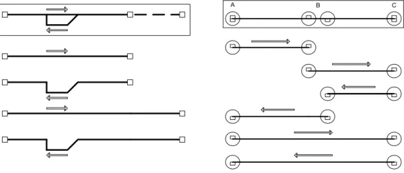
(7) The stop is made out of two boarding points (one for each direction of the 1. line for instance). Those points are in front of each other. One node has been created. 2.. Sometimes a stop is only made out of one boarding point (when the stop is only served in one direction for instance).. 3.. The boarding points for each direction are located at a non-negligible distance. In this case we created a node for each boarding point. Figure 2. Stops, boarding points and nodes. 1. 2. 3. 4. Cases. Legend Line. 4.. Node. Boarding point. Stops where different lines cross are particular cases. The stop has then generally more than two boarding points. Links are only possible in the same node (links involving walking are not considered). One node is thus created. Remember that a time of two minutes was imposed to make a connection.. 4.2. Missions and sections. A line can have different routes [Figure 3]. The public transport lines have been divided in what we call “missions”. A mission corresponds to one and only route covered by a bus line from an origin stop to a destination stop.. Figure 3. Public transport line and missions. Example: one line compounded by four missions. Figure 4. Missions and sections. For instance: two lines following the same road, the first line stops at stops A and C, the second line at stops A, B and C. The boarding points of stop B are at a non-negligible distance two nodes are thus defined. 7.

(8) A. B. C. The attributes of the sections are the mission running on them, their origin node, their destination node and the time necessary for the mission to cover them. Sections are thus directive and can be stacked [Figure 4]. 4.4. Database. The network is integrated in the database by two tables : the node tables with their name and coordinates and the section table with their code, the mission covering them, the origin and destination nodes and the time necessary for the mission to cover them. The data necessary to calculate the waiting time is the frequency. A table with the missions and their frequency has thus been created. Figure 5. Database. Nodes name coordinate x coordinate y. Sections code mission code origin node destination node covering time. Missions code frequency. The studied network is compounded with 183 nodes, 853 sections, 21 lines divided in 53 missions. 4.5. Finding for the shortest route and its alternatives. The search for the shortest route and its alternatives has been done with a Turbo Pascal program. The program can solve the following problems:. 8.

(9) -. -. search for the shortest way and its alternatives (responding to the multiple service condition) between a fixed origin and a fixed destination, an origin and all the destinations and a destination and all the origins; the search can be done at three degrees of complexity : direct links, direct links and links with one connection, and direct links and links with one and two connections. The search times increases obviously with the complexity.. The program uses two data files deriving from the database. A file with the node and the missions passing on it and another file with the missions, their frequency and the node served with the aggregated time from the origin. When an origin and a destination node are submitted to the program, the program searches the missions serving the origin node and the destination node in the corresponding table. If one or more missions are common to the origin and the destination it means that there are one or more direct links. Between those links, the program checks if they respond to the multiple service condition. Therefore each link is compared with the fastest link in terms of global route time. When the search includes the search of links with one connection, the program searches in addition to the direct links the nodes common to the missions serving the origin and the destination. The links are kept if the sum of their route time is inferior or equal to the global time of the fastest link. When the search is pushed to two connections, the program searches, (in addition to the direct links and the links with one connection) for each node served by a mission passing at the origin another mission serving this node and a node covered by a mission passing at the destination. At the end of the search the program produces a file with all the kept links. This file contains the total route time, the sum of the mean waiting times, the global time of each mission used to reach the destination, the mean waiting time of each mission, the origin node, the destination node, the connection nodes and the missions compounding the link. Such files can be very bulky. This is due to the fact that, in the case of links with one junction, each mission serving the origin node and the connection node is considered. This file is used by another routine proceeding in several stages. First, the program applies the multiple service to the links with the same origin and destination nodes. The multiple service is thus calculated on each piece of the trip (for instance: origin node to connection node and connection node to destination node). The multiple service condition is not necessary anymore because it was applied in the previous program. At the term of this stage data is obtained for each link. The results distinguish between connection nodes. Among those results, only the best one is kept (the fastest one) since it is difficult to implant a multiple service formula between direct links and links with connections. At the last stage a time for each node is obtained in the case of a search between the entire nodes and an origin or a. 9.

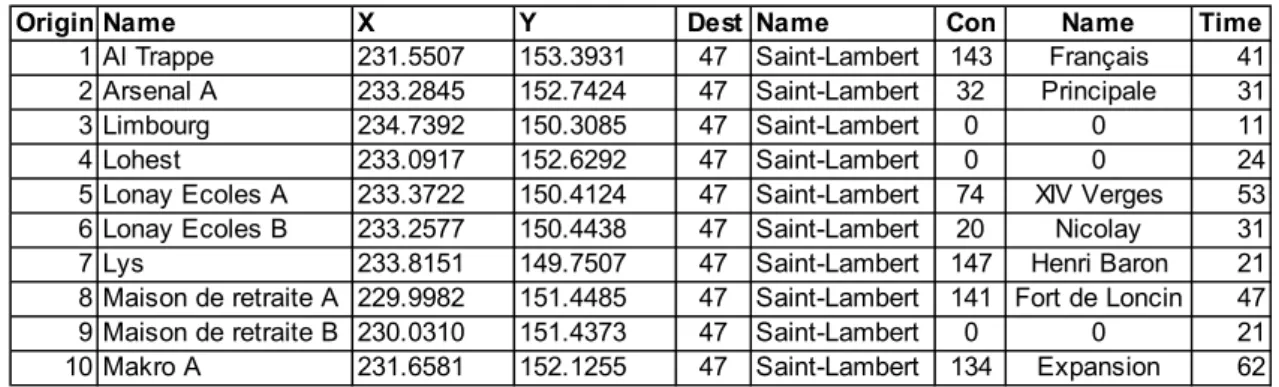
(10) destination node. This time is the mean global route time from the origin to the destination [Table 2]. Table 2. Extract of the result file Origin 1 2 3 4 5 6 7 8 9 10. 5.. Name Al Trappe Arsenal A Limbourg Lohest Lonay Ecoles A Lonay Ecoles B Lys Maison de retraite A Maison de retraite B Makro A. X 231.5507 233.2845 234.7392 233.0917 233.3722 233.2577 233.8151 229.9982 230.0310 231.6581. Y 153.3931 152.7424 150.3085 152.6292 150.4124 150.4438 149.7507 151.4485 151.4373 152.1255. Dest 47 47 47 47 47 47 47 47 47 47. Name Saint-Lambert Saint-Lambert Saint-Lambert Saint-Lambert Saint-Lambert Saint-Lambert Saint-Lambert Saint-Lambert Saint-Lambert Saint-Lambert. Con Name Time 143 Français 41 32 Principale 31 0 0 11 0 0 24 74 XIV Verges 53 20 Nicolay 31 147 Henri Baron 21 141 Fort de Loncin 47 0 0 21 134 Expansion 62. WALKING TRIP. The first an last stage of a public transport trip is generally done on foot. Travellers take the shortest way to a road and then take the shortest way to the nearest stop or at least the most interesting starting stop for their trip. The time needed for the trip depends from one person to another but 5 km/h is mostly used. So the roads must be defined, the shortest way to the nearest road and to the nearest stop. The roads have been digitised from an IGNB map at 1:25000th scale. The stops were transformed into nodes and were located and digitised on the same source map. The time necessary to go from each point of the studied area to the nearest stop can be added to the global route time necessary to reach the destination by public transport or on the contrary to the global route time from the origin stop to the nearest destination stop. With these results a map of the distribution of the public transport offer is obtained. To reach the objective The IDRISI software specialised in raster spatial analysis was used. To obtain the time necessary for this part of the public transport trip, the distance between the travellers origin (or destination) point to the nearest stop must be known. To find this distance , the distance between the road pixels and the nearest stop, and then the distance between the other pixels and the road pixels were calculated. To calculate the distance between the road pixels and the node pixels the COSTGROW algorithm was used. This algorithm creates a distance/proximity surface where distance is measured as the least effort in moving over a friction. 10.

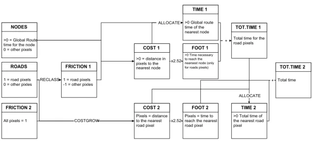
(11) surface. The distance is measured in "grid cell equivalents". A grid cell equivalent of 5 indicates the cost of moving through a grid cell when the friction equals 1. Diagonal moving increase the distance with 1.41 grid cell equivalents. We created a surface friction where the cost to move through a pixel road is 1 and –1 for all the other pixels making them impermeable. The spreading is only possible through the routes. This way, the time to go on foot to the nearest stop is the time necessary to walk through a pixel. In our case the size of a pixel is 3x3 meters. A pixel is thus crossed in 2.52 seconds at a speed of 5 km/h. When the distance is known IDRISI offers the possibility to attach each pixel to the nearest target pixel. That means that each pixel has the value of the attribute of the target pixel. In this case, the attribute is the global route time. The result of this operation is added by the SCALAR OVERLAY / ADD operation. An image with the global route time plus the time on foot for the road pixels is finally obtained. A similar operation is realised for the other pixels of the area. But the target pixels are now all the road pixels. The result image can be multiplied with a classified build/non-build image. The resulting image gives then only the values for the build pixels. This is more interesting since those pixels are the origin or destination points of the travellers. The whole IDRISI processing is exposed in the figure below. Figure 6. IDRISI processing TIME 1 ALLOCATE. NODES >0 = Global Route time for the node 0 = other pixels. ROADS 1 = road pixels 0 = other pixles. >0 Global route time of the nearest node. TOT.TIME 1 +. COST 1. FRICTION 1. >0 = distance in pixels to the nearest node. FOOT 1. Total time for the road pixels. >0 Time necessary to reach the. x2.52 nearsest node (only. TOT.TIME 2. for roads pixels). RECLASS 1 = road pixels -1 = other pixles. + Total time. ALLOCATE. FRICTION 2 All pixels = 1. COST 2 COSTGROW. FOOT 2. Pixels = distance Pixels = time to x2.52 reach the nearest to the nearest road pixel road pixel. TIME 2 >0 Total time of the nearest road pixel. 11.

(12) 6.. RESULTS. 6.1. Cases. This paragraph details two concrete cases applied to a part of the urban network of Liège. The realised maps are “from all the points to a specific destination stop” maps. The destination point of the first map is a big terminus stop in centre of the town. The phase chosen is the morning peak phase. The destination point of the second point is a stop in the centre of a secondary pole. The phase for this map is the afternoon off-peak phase. When creating such maps some node must be removed. Indeed, the nearest node does not always minimise the route time to the destination. When two boarding point of a same stop are at a certain distance two nodes were created [Figure 2]. The nearest node can thus be a node that is served by missions going in the opposite way compared with the destination. All the links were examined and such situations have been eliminated. 6.2. Analysis of the map concerning a terminus stop in the centre. The stop concerned is the Saint-Lambert Square. This square is the heart of the urban public transport system of the urban area. Most of the bus lines covering the studied area have their terminus on this square. A lot of other lines not covering our area start from there or from other nearby places. The accessibility of this square is thus fundamental. Since this place is in the downtown area, measuring the square accessibility is measuring the accessibility of the town centre. Two axes are clearly visible: the Liège-Rocourt axis and the Liège-Ans axis. Those axis are covered by many bus lines. Some of these lines have a great frequency. As consequence, the mean waiting times do not exceed seven minutes. The map shows clearly the radial disposition of the network. The secondary poles have a good link with the centre. 6.3. Analysis of the map concerning a stop in a secondary pole. In this case the stop concerned is the Astrid Square in the secondary but important pole Rocourt. This map highlights the consequence of a radial arrangement of the network. The zones near the Liège-Rocourt axis are at less than twenty minutes from destination. The zones near the Ans-Rocourt link are at less than thirty minutes. But the biggest part of the secondary pole, Ans, is more than thirty minutes away. This is due to the fact that fastest links pass through the centre where a connection must be made.. 12.

(13) Other areas near the destination are strangely at more than thirty minutes. Two reasons are at the origin of this. First, we only considered links with one junction maximum. This is justified by the fact that most of the users generally accept one connection maximum. Secondly, we have assumed that the user goes to the nearest node to take the public transport, but in some cases it is more interesting to go on foot or at least to cover a bigger distance to have a better link. Anyway this case demonstrates that two lines (19 and 88) could be extended to the Liège-Rocourt axis to improve the accessibility to the destination. 7.. IMPROVEMENTS AND FUTURE RESEARCH. The objective was to establish a method that allocates a cost-time to all the points of a given area. This time represents the mean time from the points to a specific destination or from a specific origin. Maps were conceived with this method and a analysis of the actual public transport offer has been done. The method in its actual shape has some limitations that could nevertheless beovercome Future developments of the algorithms should solve the problem resulting from comparing the connection speed of two routes to a third one (figure 7). In its actual form, if the fastest line is line 1, the connection for line 2 will take place at the same connection node as line 1 (node 1) while line 2 is also crossing line 3 at the connection node 2. This results in line 1 being advantaged over line 2 for connection with line 3. Figure 7.. Origin. 2. 3. Destination. 2. 1. 1. Connection node 1 Connection node 2. The actual way for calculating the distance to the network is a simple buffering (figure 8 A). As a result, neighbouring pixels might present big differences and the closest stop - time speaking- is not the one indicated by the simple buffer (figure 8 B). A way of improving the method consist in filtering the distance surface by a local filter. The resulting distance surface should look like figure 8 C. Figure 8.. 13.

(14) A. 1. 0. 1. 2. 3. 4. 5. 6. 6. 5. 4. 3. 2. 1. 0. 1. B. 21. 20. 21. 22. 23. 24. 25. 26. 36. 35. 34. 33. 32. 31. 30. 31. C. 21. 20. 21. 22. 23. 24. 25. 26. 27. 28. 29. 30. 31. 31. 30. 31. REFERENCES Auguste J.L. (1975) Analyse géoghraphique des transports en commun routiers dans la région liégeoise, Thesis, Géography, University of Liège, Liège, unpublished. Baudot Y. and Laloux J.-P. (1980) Les transports en commun par bus in J.A Spork et al., Liège prépare son avenir. E. Wahle, Liège, pp. 87. Cancalon et Gargaillo (1991) Les transports collectifs urbains. Quelles méthodes pour quelles stratégies ? CELSE, paris. Donnay J.-P. (1983a) Le concept d'accessibilité, quelques réflexions méthodiques et applications à la région liégeoise, Thesis, Urbanism, University of Liège, Liège, unpublished. Donnay J.-P.(1983b) Détermination d'isochrones en région liégeoise selon les moyens de transports individuels, Bulletin de la société géographique de Liège 19, pp. 41-52 Dussart F. (1939) La méthode des courbes isochrones. Son application à la ville de Liège, Travaux du séminaire de Géographie de l'Université de Liège LXVII. Dussart F. (1959) Les courbes isochrones de la ville de Liège pour 1958-1959, Travaux du séminaire de Géographie de l'Université de Liège CXXXII. Engelen G. & Brans J-P. (1980). Accessibilité du territoire. Une approche quantitative par la recherche opérationnelle, Cahiers de Géographie de Besançon 20, pp 107-142. Kummert and Vandermotten C. (1975) Analyse d'un réseau de transport publics urbains a l'aide d'un ordinateur. Application au cas de Bruxelles, Etude de géographie des transports, Amiens, France, 1975, pp. 173-177. MET - Ministère Wallon de l'équipement et des transports (1996) Transports collectifs à Liège, les grands axes d'une intégration, Coll. Trafics, 14. MET, Namur. Orfeuil J.-P. and Troulay P. (1989) Les déplacements dans le cadre habituel in INRETS (ed.) Un milliard de déplacements par semaine. La mobilité des Français, La documentation française, Paris, pp. 71-85. Roy T. (1991). Traffic Assignement Techniques, Avebury technical, Hants.. 14.

(15) Vancreaynest B. (1986) Het openbaar vervoer in het Gentse stadsgewest, Publicaties van het seminarie voor Menselijke en Ekonomische Geografie de Rijksuniversiteit te Gent 16, 116 p. Vanraes N. (1997) Analyse de la structure d’un réseau de transport en commun en vue d’une étude d’accessibilité. Application à la région d’Ans-Rocourt, mémoire de licence en sciences géographique, département de géomatique - université de Liège Liège, 213 p. i. In this paper we will use the term “bus line” which doesn’t exist in English but is used in other languages: Ligne de bus (French), linea (Italian), buslinie (German), Bus Lijn (Dutch). Those terms don’t have a translation in English. Bus route is used in Great-Britain but it refers only to the path followed.. 15.

(16)