GENERAL INTRODUCTION ... 1
LITERATURE REVIEW... 2
1. DAIRY FARMING IN NEW ZEALAND ... 2
1.1. A PASTORAL DAIRY FARMING SYSTEM... 2
1.2. ECONOMIC VIEW OF THE PASTORAL DAIRY FARMING SYSTEM... 3
1.3. BREEDS FOUND IN NEW ZEALAND... 4
1.4. ECONOMIC SITUATION OF THE DAIRY INDUSTRY IN NEW ZEALAND... 4
1.5. CONSEQUENCES FOR DAIRY CATTLE BREEDING IN NEW ZEALAND... 4
2. MATING STRATEGIES IN NEW ZEALAND ... 6
2.1. STRAIGHT BREEDING STRATEGY... 6
2.2. UPGRADING STRATEGIES... 6
2.3. CROSSBREEDING STRATEGIES... 6
2.3.1. Crossbreeding benefits... 7
2.3.2. Heterosis ... 7
2.3.3. Specific crossing schemes ... 9
2.3.4. Rotational crossing schemes ... 10
2.3.5. Crossbreeding: performances... 10
2.3.6. Profitability of crossbreeding ... 11
2.3.7. Crossbreeding between HF strains... 12
2.3.8. Crossbreeding: Future consequences ... 12
3. GENETIC MODELS ... 13
3.1. GENERAL NOTATION OF MIXED MODELS... 13
3.2. ANIMAL MODEL... 14
3.3. REPEATABILITY MODEL... 14
3.4. TEST-DAY MODELS... 15
3.4.1. Why use TDM?... 16
3.4.2. Types of TDM... 16
4. CURRENT GENETIC EVALUATION SYSTEMS FOR NEW ZEALAND DAIRY CATTLE 18 4.1. GENETIC EVALUATION SYSTEM OF PRODUCTION TRAITS... 18
4.1.1. First stage: prediction of lactation yields ... 18
4.1.2. Second stage : analysis ... 20
4.1.3. Lactation expansion ... 22
4.2. GENETIC EVALUATION SYSTEM OF LIVE WEIGHT... 24
4.3. GENETIC EVALUATION SYSTEMS OF THE LINEAR TYPE TRAITS AND SURVIVAL... 25
4.4. USE OF GENETIC GROUPS AND RELATIONSHIPS... 25
4.5. INCLUSION OF OVERSEAS INFORMATION... 26
4.6. COMPUTATIONAL METHODS... 26
4.7. BREEDING VALUES, PRODUCING VALUES AND LACTATION VALUES : RESULTS OF GENETIC EVALUATIONS 26
4.8. PRODUCTIVE EFFICIENCY: ECONOMIC INDEXES... 27
5. CONCLUSION... 29
MATERIAL AND METHODS... 30
1. INTRODUCTION... 30
2. DATA PREPARATION ... 30
2.1. INTRODUCTION... 30
2.2. INITIAL DATA FILES... 30
2.2.1. Lactation yield details file... 30
2.2.2. Production file ... 31 2.2.3. Breed file... 31 2.2.4. Pedigree file ... 31 2.3. PREPARATION OF DATA... 31 2.3.1. Selection of lactations ... 31 2.3.2. Stratification of herds ... 31
2.3.3. Data for estimation of (co)variance components for purebred HF and JE ... 32
2.3.4. Data for estimation of (co)variance components across HF and JE ... 32
2.3.5. Data for genetic evaluation... 32
2.3.6. Additional data preparation steps... 33
2.3.7. Pedigree extraction and renumbering of effects ... 33
3. ESTIMATION OF (CO)VARIANCE COMPONENTS ... 34
3.1. (CO)VARIANCE COMPONENT ESTIMATION... 34
3.2. MODELS USED FOR ESTIMATION... 34
3.2.1. Model for estimation of (co)variance components for purebred HF and JE ... 34
3.2.2. Model for estimation of (co)variance components across HF and JE ... 35
3.3. ESTIMATION... 37
4. ESTIMATION OF BREEDING VALUES ... 38
4.1. (CO)VARIANCE COMPONENTS AND MODEL. ... 38
4.2. ESTIMATION OF EFFECTS... 39
4.3. BREEDING VALUES ESTIMATED: ANALYSIS... 39
RESULTS AND DISCUSSION ... 40
1. INTRODUCTION... 40
2. DESCRIPTION OF THE DAIRY POPULATION... 40
2.1. POPULATION OF ANIMALS IN FIRST LACTATION... 40
2.2. POPULATION USED FOR GENETIC EVALUATION... 40
3. ESTIMATION OF (CO)VARIANCE COMPONENTS FOR PUREBRED HERDS ... 42
3.1. RESULTS... 42
3.1.1. (Co)variance components estimation... 42
3.1.2. Heritabilities ... 46
3.2. DISCUSSION AND CONCLUSION... 48
4. ESTIMATION OF (CO)VARIANCE COMPONENTS ACROSS HF AND JE ... 50
4.1. MODEL I ... 50
4.1.1. (Co)variance components estimation... 50
4.1.2. Heritabilities ... 51
4.1.3. Correlations ... 51
4.2. MODEL II... 52
4.2.1. (Co)variance components estimation... 52
4.2.2. Heritabilities. ... 55
4.2.3. Correlations ... 56
4.3. COMPARISON BETWEEN MODELS I AND II ... 57
5. COMPARISON BETWEEN RESULTS FOR PUREBRED AND ACROSS BREEDS ... 59
5.1. VARIANCE COMPONENTS ESTIMATION... 59
5.2. HERITABILITIES... 61
5.3. CORRELATIONS... 61
5.4. DISCUSSION AND CONCLUSION... 61
6. GENETIC EVALUATION ... 63
6.1. MODEL II WITH DIFFERENCES BETWEEN BREEDS... 63
6.2. MODEL III WITHOUT DIFFERENCES BETWEEN BREEDS... 66
6.3. SIRES RANKING... 69
6.4. HETEROSIS AND RECOMBINATION LOSS EFFECTS... 71
CONCLUSION AND IMPLICATIONS... 73
TABLE 1:HETEROSIS EFFECTS IN PERCENTAGE. ... 9
TABLE 2:BREED AVERAGE FOR MILK RECORDED COWS IN 2002-2003. ... 11
TABLE 3:CONTRIBUTIONS FOR SOLVING THE MME BY ITERATION ON DATA METHODS. ... 24
TABLE 4:COMPOSITION OF SAMPLES. ... 33
TABLE 5:MEAN BREED COMPOSITIONS OF POPULATION OF ANIMALS IN FIRST LACTATION. ... 40
TABLE 6:COMPOSITION OF POPULATION USED FOR THE GENETIC EVALUATION... 41
TABLE 7:(CO)VARIANCE COMPONENTS (LITRES²) FOR MILK ESTIMATED FOR HF PUREBRED HERDS... 42
TABLE 8:(CO)VARIANCE COMPONENTS (LITRES²) FOR MILK ESTIMATED FOR JE PUREBRED HERDS... 43
TABLE 9:VARIANCES AND HERITABILITIES CALCULATED ON 270DIM FOR PUREBRED HERDS. ... 45
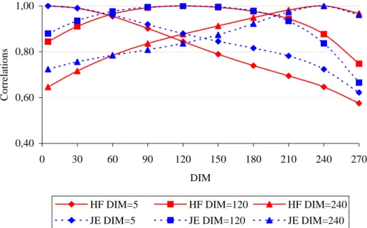
TABLE 10:HERITABILITIES, GENETIC CORRELATIONS AND PHENOTYPIC CORRELATIONS FOR MILK AMONG FIRST LACTATION ESTIMATED FOR HF PUREBRED HERDS... 47
TABLE 11:HERITABILITIES, GENETIC CORRELATIONS AND PHENOTYPIC CORRELATIONS FOR MILK AMONG FIRST LACTATION ESTIMATED FOR JE PUREBRED HERDS... 48
TABLE 12:(CO)VARIANCE COMPONENTS (LITRES²) FOR MILK ESTIMATED FOR CROSSBRED HERDS USING MODEL I. ... 50
TABLE 13:VARIANCES AND HERITABILITIES CALCULATED ON 270DIM FOR PUREBRED AND CROSSBRED ANIMALS USING MODEL I(CROSSBRED HERDS)... 51
TABLE 14:CORRELATIONS BETWEEN HF AND JE BREEDS ESTIMATED FROM MODEL I... 51
TABLE 15:(CO)VARIANCE COMPONENTS (LITRES²) FOR MILK ESTIMATED FOR CROSSBRED HERDS USING MODEL II. ... 52
TABLE 16:VARIANCES AND HERITABILITIES CALCULATED ON 270DIM FOR PUREBRED AND CROSSBRED ANIMALS USING MODEL II(CROSSBRED HERDS)... 54
TABLE 17:HERITABILITIES (DIAGONAL), GENETIC CORRELATIONS (ABOVE DIAGONAL) AND PHENOTYPIC CORRELATIONS (BELOW DIAGONAL) FOR MILK AMONG FIRST LACTATION ESTIMATED FOR HF=1 ANIMALS. 56 TABLE 18:HERITABILITIES (DIAGONAL), GENETIC CORRELATIONS (ABOVE DIAGONAL) AND PHENOTYPIC CORRELATIONS (BELOW DIAGONAL) FOR MILK AMONG FIRST LACTATION ESTIMATED JE=1 ANIMALS. ... 56
TABLE 19:HERITABILITIES (DIAGONAL), GENETIC CORRELATIONS (ABOVE DIAGONAL) AND PHENOTYPIC CORRELATIONS (BELOW DIAGONAL) FOR MILK AMONG FIRST LACTATION ESTIMATED FOR CROSSBRED ANIMALS (0.5HF0.5JE)... 57
TABLE 20:CORRELATIONS BETWEEN HF AND JE BREEDS ESTIMATED FROM MODEL II. ... 57
TABLE 21:SUMMARY STATISTIC FOR BREEDING VALUES (LITRES) ESTIMATED FOR MILK USING MODEL II. ... 63
TABLE 22:SUMMARY STATISTIC FOR FITTED BREEDING VALUES (LITRES) ESTIMATED FOR MILK USING MODEL II. ... 64
TABLE 23:SUMMARY STATISTICS FOR FITTED BREEDING VALUES (LITRES) BY “BREED” FOR COWS IN PRODUCTION. ... 65
TABLE 24:SUMMARY STATISTICS FOR FITTED BREEDING VALUES (LITRES) ESTIMATED FOR MILK USING MODEL III. ... 67
TABLE 25:SUMMARY STATISTICS FOR “AVERAGE” BREEDING VALUES (LITRES) COMPUTED FOR MILK. ... 68
TABLE 26:SPEARMAN RANK CORRELATION AND BREEDING VALUES FOR SIRES USING MODEL II... 69
TABLE 27:SPEARMAN RANK CORRELATION AND “AVERAGE” BREEDING VALUES FOR SIRES USING MODEL III.... 70
TABLE 28:TOP 10 OF SIRES FOR THE THREE BREEDING VALUES... 71
TABLE 29:HETEROSIS AND RECOMBINATION LOSS ESTIMATED USING MODELS II AND III. ... 71
FIGURE 1:REPRESENTATION OF DAILY PASTURE GROWTH AND DAILY HERD FEED REQUIREMENT IN FUNCTION OF
MONTHS [PRYCE AND HARRIS,2004]. ... 3
FIGURE 2:REPRESENTATION OF SEASONAL FARMING SYSTEM IN NEW ZEALAND [PRYCE AND HARRIS,2004]. ... 3
FIGURE 3:AVERAGE MILK YIELD DURING THE LACTATION FOR ANIMALS USED FOR GENETIC EVALUATION... 41
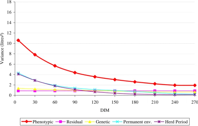
FIGURE 4:VARIANCE COMPONENTS FOR MILK AS FUNCTION OF DIM ESTIMATED FOR HF PUREBRED HERDS. ... 44
FIGURE 5:VARIANCE COMPONENTS FOR MILK AS FUNCTION OF DIM ESTIMATED FOR JE PUREBRED HERDS. ... 44
FIGURE 6:COMPARISON BETWEEN ADDITIVE GENETIC AND HERD PERIOD VARIANCES FOR MILK AS FUNCTION OF DIM ESTIMATED FOR HF AND JE PUREBRED HERDS... 45
FIGURE 7:HERITABILITIES FOR MILK AS FUNCTION OF DIM ESTIMATED FOR HF AND JE PUREBRED HERDS. ... 46
FIGURE 8:GENETIC CORRELATION CURVES BETWEEN DIM(5,120 AND 240) AS FUNCTION OF DIM ESTIMATED FOR HF AND JE PUREBRED HERDS... 47
FIGURE 9:VARIANCE COMPONENTS FOR MILK AS A FUNCTION OF DIM ESTIMATED FOR HF=1 AND JE=1 (PUREBRED) ANIMALS USING MODEL II(CROSSBRED HERDS)... 53
FIGURE 10:PHENOTYPIC VARIANCES FOR MILK AS FUNCTION OF DIM ESTIMATED FOR PUREBRED AND CROSSBRED ANIMALS USING MODEL II(CROSSBRED HERDS)... 54
FIGURE 11:HERITABILITIES FOR MILK AS FUNCTION OF DIM ESTIMATED FOR PUREBRED AND CROSSBRED ANIMALS USING MODEL II(CROSSBRED HERDS). ... 55
FIGURE 12:PERMANENT ENVIRONMENT VARIANCES FOR MILK AS FUNCTION OF DIM ESTIMATED FOR HF AND JE PUREBRED ANIMALS USING MODEL P AND MODEL II... 59
FIGURE 13:HERD PERIOD VARIANCES FOR MILK AS FUNCTION OF DIM ESTIMATED FOR HF AND JE PUREBRED ANIMALS USING MODEL P AND MODEL II. ... 60
FIGURE 14:ADDITIVE GENETIC VARIANCES FOR MILK AS FUNCTION OF DIM ESTIMATED FOR HF AND JE PUREBRED ANIMALS USING MODEL P AND MODEL II... 60
FIGURE 15:HERITABILITIES FOR MILK AS A FUNCTION OF DIM ESTIMATED FOR HF AND JE PUREBRED ANIMALS. ... 61
FIGURE 16:GENETIC TREND OF COWS IN PRODUCTION COMPUTED USING MODEL II. ... 64
FIGURE 17:GENETIC TREND FOR MILK BY BREED FOR FITTED BVHF. ... 65
FIGURE 18:GENETIC TREND FOR MILK BY BREED FOR FITTED BVJE. ... 66
FIGURE 19:HERITABILITIES FOR MILK AS FUNCTION OF DIM ESTIMATED FOR CROSSBRED HERDS USING MODEL II AND FOR BASIS ANIMAL USING MODEL III... 67
FIGURE 20:GENETIC TREND OF COWS IN PRODUCTION COMPUTED USING MODEL III... 68
FIGURE 21:EVOLUTION OF MEAN HETEROSIS AND MEAN RECOMBINATION LOSS ACROSS YEARS ESTIMATED FOR COWS IN PRODUCTION USING MODEL II AND MODEL III. ... 72
GENERAL INTRODUCTION
Crossbreeding is a method used for improvement in agricultural industries such as pigs, beef cattle and poultry but it is not usual for dairy cattle in most temperate countries, due to the high milk production of the Holstein-Friesian breed. The exception is New Zealand where widespread adoption of crossbreeding has been a feature of the recent history of the dairy industry and now more than one third of the replacement cattle are crossbred.
Under New Zealand pastoral conditions where the objective is to maximize the net income per hectare, crossbreeding can provide a good opportunity. Moreover, it allows to improve composition of milk that is an important feature since farmers are paid on the basis of quantity of milk solids (fat and protein) and not of milk yield. Thus, crossbreeding permits to increase the farm net income
Since 1996, an across-breed genetic evaluation system for milk, fat and protein yields, using a two-step test-day model, has been used to compare animals nationally and within herd regardless of breed.
Actually, a test-day random regression model is under development for the genetic evaluation of somatic cell count and will be implemented in 2005. A random regression test-day model allows to model more correctly the shape of lactation by use of polynomials of time, so it provides a better representation of the biological lactation curve.
The objective of this work was to contribute to development of such a model for the genetic evaluation of production traits (milk, fat and protein) in New Zealand and allowing to take breed differences in an optimal manner into account. In order to do this a advanced model was developed allowing breed specific additive genetic effects. Needed (co)variance components were estimated first inside purebreds then across breeds. Based on this model, breeding values were estimated and rankings of sires compared. The results provided a first test of the feasibility and the usefulness of a random regression test-day model with breed specific additive genetic effects.
LITERATURE REVIEW
1. Dairy farming in New Zealand
1.1. A pastoral dairy farming system
Breeding of dairy cows in New Zealand consists in an extensive grazing system, with pastures of several hectares where cows are largely fed on grass. The New Zealand climate allows that cows to spend their entire lives outside in most of the areas, therefore they must be able to perform at temperatures ranging from below zero to 40 degrees Celsius, and continue to produce milk from often minimal pasture. But in colder areas of New Zealand (next to the Southern Alps for example), they may be sheltered or fully housed during the winter months. They must also have a good conformation with strong legs, excellent feet and udders that are well developed and strongly supported because they walk daily long distances to be milked. Thus cows must settle quickly into their milking routine, have a mild temperament and are fast through the milking shed. Cows that do not exhibit these traits or a good conformation are quickly culled as are the bulls that sired them [Meadows, 1996].
In this system the main component of cows diet is grazed pasture and pasture products; concentrate is rarely fed and the quantities of hay and silage (maize or grass) fed per cow are low in comparison with European and North American dairying systems. This is due to unfavorable grain prices compared to milk prices [Harris and Kolver, 2001]. Approximately fourteen million tonnes of pasture dry matter is utilized annually for conversion into thirteen million tonnes of milk [Montgomerie, 2003].
Their first calving happens often when they are around two years old and they continue to calve each year for life. The seasonal nature of the farming system demands that every cow should have a calving interval close to 365 days, cows not respecting this interval are culled resulting in an indirect selection on cows fertility at the farm level. Most of calving take place in a window of eight weeks in the late winter or early spring, generally between July and September-0ctober coincident with the period of rapid grass growth (Figures 1 and 2). But a small number of farmers choose to be “winter milk farmers”, their cows calving in the late summer and autumn (March to May) to produce milk through the winter months. Moreover, sometimes cows in New Zealand can have induced lactation1 that is the pregnancy is terminated up to four weeks before planned calving date [Harris, 1994].
1
This practice yields an unfavorable effect, the milk yield depression due to this is close to 4-5% of the annual yield. [Harris et al., 1996]
As the average New Zealand dairy farmer need to calve over 250 cows in an eight week period, it is obviously essential to minimize calving difficulties [Meadows, 1996]. The cows are dried off in late summer or autumn, depending on climatic conditions such as rainfall, so that the reduced feed requirements of dry cows coincide with winter when pasture growth is at its slowest [Harris and Kolver, 2001] (see Figures 1 and 2).
Thus on average, the term of lactation is 225 to 250 days that is due to New Zealand dairy grazing system. Figures 1 and 2 represent this seasonal farming system based on pastures.
Figure 1: Representation of daily pasture growth and daily herd feed requirement in function of months [Pryce and Harris, 2004].
Figure 2: Representation of seasonal farming system in New Zealand [Pryce and Harris, 2004].
1.2. Economic view of the pastoral dairy farming system
The objective of pasture based farming is to maximise the net income per hectare rather than per cow [Harris, 1998]. In fact, income per cow as a measure fails to account for the large variation between achievable stocking rates for herds with substantially different live weight and milk yield characteristics. Stocking rate2 is the number of milking cows per hectare of productive land. So, the total milk production per unit of feed consumed in this pastoral system is a function of the average animal production, genetic improvement and stocking rate. In the current situation, the stocking rate is 2.61 cows per hectare and the average herd size is 285 cows by herd [Montgomerie, 2003].
Thus, the net farm income is related to production per hectare of available grazing land. This low-cost system is supported by a climate that allows pasture to grow year round, even if it is a marked seasonal pattern.
2
Computed as the ratio of utilizable pasture per hectare to the total dry matter requirement (including replacements) per cow per year. [Lopez-Villalobos and Garrick, 1996]
1.3. Breeds found in New Zealand
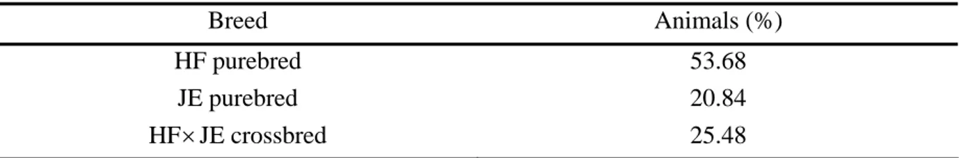
The most common breed in New Zealand is Holstein-Friesian but more than one third of the replacement cattle bred for the dairy industry are crossbred and is increasing. So, the percentages of breeds and crosses in the current dairy population, which counts approximately 3.7 million of cows, are 52% Holstein-Friesian, 24% Holstein-Friesian×Jersey crossbred, 15% Jersey, 6% other crosses (include three breed crosses) and 3% other breeds mainly Ayrshire. [Montgomerie, 2003; Harris, 2004]
Most of the dairy herds in New Zealand are a mixture of purebred and crossbred cows [Lopez-Villalobos et al., 2000c].
1.4. Economic situation of the dairy industry in New Zealand
In New Zealand, the dairy industry is oriented towards export production; 90%-96% of the milk is manufactured into a range of dairy products and exported to many countries. Few cows are required to supply fluid milk to domestic consumers [Harris, 2004; Montgomerie, 2003].
Low cost systems for conversion of pasture into protein and fat (milk solids) provide the basis for the industry to survive [Lopez-Villalobos et al., 2000a, 2000c]. Generally, farmers are rewarded for the amount of protein and fat produced, with a penalty made for milk volume produced. This penalty allows the dairy industry to face up to transporting, storing and processing costs [Montgomerie, 2003]. Moreover, the value of payment is determined by the prices for which milk products are sold to the world market minus costs of processing and marketing. Often, the milk price for producers is typically around half the producer price received by EU and USA producers [Montgomerie, 2002].
In the face of the low milk prices, most operators achieve acceptable profitability by spending only small amounts on purchased feed, and by managing high numbers of cows for each staff member (around 150-200 cows per staff member) [Montgomerie, 2003].
1.5. Consequences for dairy cattle breeding in New Zealand
This special situation has obviously repercussions on dairy cattle breeding in New Zealand and leads to different breeding objective and favors the selection of animals that are well adapted for this type of management (e.g. easy calving, high fertility). Another method to improve the value of milk is provided by crossbreeding and selection which allow to modify yield of milk and its components (fat and protein). Indeed, farm costs can be reduced if the same amount of milk solids is produced per hectare by a smaller number of cows. Milk collection and manufacturing costs can be reduced too if the same amount of milk solids is processed from a smaller volume of milk. Thus, crossbreeding is an option to increase farm profit [Lopez-Villalobos and Garrick, 1997b; Lopez-Villalobos et al., 2002].
Several studies done in New Zealand over the past few years [e.g. Lopez-Villalobos and Garrick, 1996; Lopez-Villalobos et al., 2002; Lopez-Villalobos and Garrick, 2002] evaluated the effect of selection and mating strategies on industry production of milk components and dairy industry net income (see part Profitability of crossbreeding).
2. Mating strategies in New Zealand
Mating strategies affect breed composition in New Zealand and therefore productivity of the whole dairy industry. There are three kinds of mating strategies in New Zealand involving Holstein-Friesian (HF), Jersey (JE) and Ayrshire (AY) breed : straight breeding, upgrading or grading-up and crossbreeding. These mating strategies influence gene combinations received by the progeny; they were evaluated for several breed combinations in different studies.
2.1. Straight breeding strategy
The goal of this strategy is to avoid crossbreeding and allows to maintain purebred (HF, JE and AY) composition of national herd. Moreover, straight bred herds produce their own replacements by mating the cows to bulls of the same breed [Lopez-Villalobos and Garrick, 1997b]. This mating system is important because it allows to supply purebred bulls and cows of high genetic merit used in crossbreeding and upgrading strategies [Lopez-Villalobos et al., 2000a].
According to Dairy statistics for the 2002-2003 season in New Zealand, HF cows produced more milk, fat and protein than JE cows. However, milk from JE is more concentrated in fat and protein for a smaller volume of milk.
2.2. Upgrading strategies
The aims of these strategies are to create one dominant breed in the population by continuous mating of females to males of the expected dominant breed. After five generations, the progeny theoretically have 96.9% of their genes from dominant breed [VanVleck et al., 1987].
2.3. Crossbreeding strategies
The use of crossbreeding is common in agricultural industries such as pigs and poultry but has been widely ignored in dairying in most of temperate countries. Indeed, crossbreeding in dairy cattle has not been widespread in temperate climates, largely because of the notable merit of the HF breed for liquid milk production [Touchberry, 1992].
The exception is in New Zealand, where crossbreds are now the second largest “breed type” at approximately 25% of the dairy cow population. Since 1985, crossbreeding is actively practiced by dairy farmers and the interest in crossbreds is so strong in New Zealand that crossbreds bulls are now being progeny tested (Kiwicross bulls) [Montgomerie, 2002].
2.3.1. Crossbreeding benefits
Crossbreeding is a system of mating individuals from different breeds; it is a kind of process in which the gene flow is very important and therefore it produces positive results due to two main effects.
First, it is the ability to utilize complementarity, a well-designed crossbreeding system allows the producer to combine the desirable characteristics of the breeds involved in the cross while masking some of the disadvantages of the breeds. For example, HF produce a high milk volume and JE produce high milk components; by crossing these two breeds the producer aims to produce an animal that produces a large volume of milk that also contains a high component content [Falconer, 1989]. Breed complementarity can generate economic advantage in crossbred animals even in the absence of heterosis for individual traits [Lopez-Villalobos and Garrick, 2002].
The second effect arises from heterosis or hybrid vigor and it can lead to economic gains through heterosis [Swan and Kinghorn, 1992] (see part about heterosis).
Crossbreeding also takes advantage of the increase of heterozygosity that it produces and so it can be considered as a solution to increasing levels of inbreeding within each of the major dairy breeds [Swan and Kinghorn, 1992]. Indeed, according to VanRaden [1992], crossbreds are more heterozygous and less inbred than purebreds, only crossbreds may have an inbreeding coefficient of zero.
Moreover, the crossbreeding strategies can provide an opportunity to make progress in one generation that would require generations of selection to obtain it and can allow the introduction of a new breed in a herd [Bidanel, 1992].
In conclusion, all these reasons can lead to an increase of overall productivity. Nevertheless, crossbreeding is not a cure for inferior management and cannot replace the need for continued selection policies in the “purebred” herds.
2.3.2. Heterosis
When two different populations are crossed causing an increase in heterozygosity in F1 generation, the level of inbreeding in the hybrid falls to zero and there is an improvement in the traits which suffered from inbreeding depression in the parents populations. This improvement is called heterosis or hybrid vigor, it is the phenomenon in which progeny of cross is better than the expected average of the two populations for a particular trait [VanVleck et al., 1987].
According to VanRaden [1992] heterosis can be considered being the opposite of inbreeding depression, therefore the extra performance observed through heterosis is simply
the recovery of losses that occurred through inbreeding depression over time in the parental breeds. In this way, inbreeding and heterosis can be modeled on the same scale.
Biological explanations
Heterosis is usually attributed to non-additive genetic interactions within loci (dominance) and interactions between loci (epitasis). Indeed, it is mainly caused by dominance complementation or over dominance due to pleitropic effects. Dominance is present if the heterozygous individual is not exactly intermediate between the two homozygotes [Falconer, 1989]. The amount of heterosis gain depends on the difference in gene frequencies at loci where dominance effects exists in the two breeds. However, epistasis may also play a part in heterosis, the consequence of these epistatic effects is that the prediction of heterosis level due to heterozygosity will be biased because it is difficult to model the epistatic effects and so to predict them [Panicke and Freyer, 1992; VanVleck et al., 1987].
Measurement
Heterosis is typically measured as a deviation from the average of the parental breeds, and it is expressed on a percentage of their parent’s performance [VanVleck et al., 1987]:
100 average Parent average Parent average Crossbred Heterosis % = − × (1)
According to preceding equation, heterosis is measured as the deviation of crossbred progeny from what is expected from a completely additive genetic model, thus it is the non-additive component of crossbreeding.Not all traits express the same degree of heterosis, there is a considerable improvement in traits due to the heterosis, most noticeably in low heritability traits like fertility and survival than in moderate heritability traits like milk production [VanRaden, 1992]. Furthermore, the degree of heterosis for the same trait varies between strains, breeds and environments [Swan and Kinghorn, 1992]. It is very difficult to predict accurately just how much heterosis to expect from a given cross. But the mean performances of a crossbred can be predicted knowing the performance and degree of heterosis of the breeds crossed.
Heterosis in New Zealand
Several studies [Ahlborn-Breier, 1989; Ahlborn-Breier and Hohenboken, 1991; Panicke and Freyer, 1992; Harris et al., 1996] on the national data have revealed positive heterosis effects for production traits, for live weight, for fertility and for survival, these facts can explain the increase of crossbreeding in New Zealand. Expressed in percentage terms, the average first cross heterosis effects estimated from the New Zealand national data 1986-1995 are shown in Table 1.
Table 1: Heterosis effects in percentage.
Traits HF×JE HF×AY JE×AY
Fat yield 4.3 1.8 5.0
Protein yield 4.2 1.9 4.7
Milk volume yield 4.1 1.8 4.8
Liveweight 1.7 0.8 3.1 Fertility 6.8-10.1* NA NA Survival (1st to 2nd lactation) 3.4-8.8 * 2.6 4.7
* estimated heterosis effects for local HF strain×JE and for overseas HF strain×JE (Source: Montgomerie, 2002)
Loss of heterosis
First generation crossbred animals express 100% of the heterosis. In the next generation, these favourable combinations of genes from each breed will be mixed up with genes from the other breed(s). So, subsequent crosses will still produce some heterosis but to a less extent. This decrease of heterosis is called recombination loss or heterosis loss and it due to dominance for a part but epistasis may lead to increase or decrease this loss. This loss is one reason why second and later generation crosses usually do not perform as well as the first generation cross. Estimates for recombination loss vary widely over literature, but generally the effect is negative and smaller than the effect of heterosis in absolute value [Van Der Werf, 1990; Lopez-Villalobos, 1998].
However, some crossbreeding schemes can maintain high levels of heterosis such as rotational crossing schemes. Indeed, the average milk solids yields of the first reciprocal crosses and of the ¾ HF backcross cows exceeded the average milk solids yield of the HF cows [Lopez-Villalobos and Garrick, 1997; Montgomerie, 2002].
2.3.3. Specific crossing schemes
These schemes indicate mainly first-cross or F1 between two purebred animals. The F1 contains 50% of genes of the two parental breeds and expresses 100% of the heterosis [Lopez-Villalobos and Garrick, 1997b].
The high productivity of F1 cows comprising HF and JE breeds have been identified by several studies in New Zealand [Ahlborn-Breier, 1989; Ahlborn-Breier and Hohenboken, 1991; Lopez-Villalobos and Garrick, 1997b; Lopez-Villalobos et al., 2000c]. Ideally the whole herd should be made up of first-cross animals but these animals cannot produce their own replacements unless some purebred animals are maintained. Thus, one approach for
exploiting heterosis in a self-replacing herd is by the way of rotational crossbreeding [Lopez-Villalobos et al., 2000a].
2.3.4. Rotational crossing schemes
Purebred bulls of different breeds are mated to crossbred cows from alternate generations. Rotational crossbreeding allows to exploit additive and heterosis effects in self-replacing herds and to maintain high levels of heterosis in animals [Lopez-Villalobos and Garrick, 1996, 1997b; Lopez-Villalobos et al, 2000a].
In a two-breed rotational scheme with HF and JE, starting with a JE herd, cows are mated to HF bulls to produce F1 HF × JE cows. Half of the F1 cows are mated to HF bulls to
produce ¾ HF ¼ JE cows, and the other half are mated to JE bulls to produce ¼ HF ¾ JE cows. Next, ¾ HF ¼ JE cows are mated to JE bulls and ¼ HF ¾ JE cows are mated to HF bulls. After three more generations, half of the herd will be 2/3 HF 1/3 JE and the other half will be 1/3 HF 2/3 JE. This strategy can retain two thirds (67%) of the original heterosis expressed by the F1. Similar approaches can be followed for two-breed rotation with HF and
AY and with JE and AY [Lopez-Villalobos et al., 2000a].
In a three-breed rotational scheme with HF, JE and AY, starting with an AY herd, cows are mated to JE bulls to produce F1 JE × AY cows. These F1 cows are mated to HF
bulls to produce ½ HF ¼ JE ¼ AY, which will be mated to AY bulls to produce ¼ HF 1/8 JE 5/8 AY, and so on. After several generations, the herd will comprise three groups of animals: 4/7 HF 2/7 JE 1/7 AY, 2/7 HF 1/7 JE 4/7 AY and 1/7 HF 4/7 JE 2/7 AY. Heterosis decreases also in each generation but at equilibrium 86% of the original heterosis can be observed [Lopez-Villalobos et al., 2000a].
2.3.5. Crossbreeding: performances
Results from different studies [Villalobos and Garrick, 1996; 1997b; Lopez-Villalobos, 1998; Lopez-Villalobos et al., 2000a, 2000b] indicated that crossbred cows are more productive than purebred cows. On average, HF×JE crossbred cows produce less milk volume but with high concentrations of fat and protein than purebred HF. The body size and live weight of these crossbred animals is smaller than HF animals therefore stocking rate increases but it is smaller than JE stocking rate [Montgomerie, 2002]. These animals are also more adapted to an extensive system than HF and so have a better efficiency to convert pasture into prime milk.
Moreover, according to some studies [Grosshans et al., 1997; Harris and Winkelman, 2000; Lopez-Villalobos et al., 2000b] crossbred cows had a better fertility.
According to the milk recording statistics, for the main breeds and crosses in the 2002-2003 season, crossbred cows produced more fat than both parent breeds and than AY cows
while HF cows produced more protein and a higher volume of milk. Table 2 shows these milk recording statistics.
Table 2: Breed average for milk recorded cows in 2002-2003.
Breed Number Milk (litres) Fat (kg) Protein (kg)
HF 1,110,878 4038 175.4 142.9
JE 374,409 2839 162.6 116.9
HF×JE * 612,868 3610 179.1 137.3
AY 25,880 3571 154.9 128.6 * includes backcrosses.
(Source: Dairy Statistics 2002-2003)
Most authors observed clear benefits for first-cross HF x JE cows and for profitable use of rotational crossbreeding systems [e.g. Lopez-Villalobos and Garrick, 2002].
2.3.6. Profitability of crossbreeding
Results from several studies [e.g. Villalobos and Garrick, 1996, 1997b; Lopez-Villalobos et al., 2002; VanRaden and Sanders, 2001] have suggested that crossbreeding could increase net returns of the farm.
According to Lopez-Villalobos and Garrick [1997a] crossbred cows tended to be more profitable than purebred cows because they fitted the milk payment system and showed favourable heterosis for milk traits. So, net income per hectare was higher for crossbred cows than for purebred HF or JE cows.
In a study, investigators in New Zealand have sought to evaluate the profitability of alternative breeding systems under pastoral conditions. Lopez-Villalobos et al. [2000a] developed a comprehensive deterministic model based on a 25 year planning horizon which on an annual basis simulated nutritional, biological and economic performance of straight breeding and rotational crossbreeding using two or three New Zealand breeds. Breed additive effects and heterosis for milk, fat and protein yields, body weight and survival were taken from analyses of field data in New Zealand. The economic analysis revealed the largest advantage in net income per hectare3 for a HF-JE rotational cross which was only slightly larger than that for a HF-JE-AY rotational cross. Results were similar for net income per cow. For milk income, HF and the rotational cross groups were nearly identical. Results of this study suggested that, under New Zealand conditions, the use of rotational crossbreeding systems could increase profitability of dairy herds under the conceivable market conditions. Moreover, the two-breed rotational scheme with HF and JE seems to be an alternative mating
3
Net income per hectare is a more important measurement of economic effiency than is net income per cow for New Zealand dairy farmers.
strategy to exploit variation within and between breeds for milk production through a stratified breeding scheme combining selection and crossbreeding as methods of genetic improvement. These results were confirmed by a recent study realized by Lopez-Villalobos and Garrick in 2002.
However, future costs and prices of dairy products (economic circumstances) have major impact on profit of mating strategies. More information are available in Lopez-Villalobos et al. [2000c] and in Lopez-Lopez-Villalobos and Garrick [2002].
Furthermore, crossbreeding can benefit traits such as reproduction (fertility), health and survival, which sometimes have large influences on farm profit [e.g. Touchberry, 1992; Lopez-Villalobos et al., 2000b; White, 2002].
2.3.7. Crossbreeding between HF strains
Crossbreeding between the local HF strain (NZHF) and the overseas HF strain (IHF) has occurred since 1980 as artificial insemination companies introduced North American genes into their breeding schemes. However, this crossbreeding program within the HF breed is not deliberately followed by farmers in opposition to crossbreeding between HF and JE purebreds [Montgomerie, 2002]. Moreover, heterosis from crossbreeding between IHF and JE is more important than heterosis from NZHF×JE because IHF strain is more genetically different of the JE breed [Harris and Kolver, 2001; Pryce and Harris, 2004].
2.3.8. Crossbreeding: Future consequences
Lopez-Villalobos et al. [1997; 2000b] carried out some studies evaluated the effects of simultaneous selection and mating strategies (upgrading and rotational crossbreeding) on the rate of genetic improvement and productivity of the New Zealand dairy cattle with a deterministic model based over a 25 year planning horizon. For all mating strategies, the size of active cow population affected the within-breed average annual genetic gain. Therefore, the adoption of rotational crossbreeding reduced the size of the potential purebred bull mothers4 population with only minor changes in the annual genetic gain of bulls compared to upgrading strategies. However, annual recruitment of new active cows should be regularly monitored to ensure long term gain will be maintained [Lopez-Villalobos and Garrick, 1997b].
Therefore, in the long term, crossbreeding can be used in combination with selection to exploit the effects of heterosis while maintaining genetic diversity to cover changes in market conditions [Lopez-Villalobos et al., 2000b].
4
Also known as active cows that may be registered (pedigree) or not (grade), provided that they are the result of at least three generations of artificial breeding to sires of one breed.
3. Genetic models
Dairy cattle breeding aims to reduce the production costs of milk, improve animal health and welfare, thus to increase farm profitability by improving the genetic level of livestock. This is most effectively achieved by selection of animals with the highest genetic merit, using accurately breeding values which allow to compare and to classify animals between them. Breeders operate on these breeding values, which are solutions to mixed model equations (MME) established by Henderson.
3.1. General notation of mixed models
Henderson adapted theories of linear models to quantitative genetic. According to Henderson [1984] a mixed linear model can be written in matrix notation as:
e Zu Xb
y= + + (2)
where y is the vector with all the observations; b is the vector with unknown fixed effects; u is the vector with unknown random effects; X is the incidence matrix which relates observations to corresponding fixed effects; Z is the incidence matrix which relates observations to corresponding random effects; e is the vector of the residuals. With this model, the mean of y is represented by Xb since both random effects and residuals have a mean of zero and the covariance between its observations by Var(y)=Var(Xb) + Var(Zu) + Var(e). However, V(Xb)=0 since b is a fixed effect, Var(u)=G and so Var(Zu)=ZGZ’ and Var(e)=R then Var(y)=V=ZGZ’ + R, with the assumption that the random effect and the residual are not correlated, thus Cov (u, e)=0.
The resolution of equation (2) provides the following solutions [Henderson, 1984]: y V X' X V X' bˆ=( −1 )−1 −1 (3) ) ( ˆ GZV y Xb u= −1 − (4)
However, this resolution requires the inversion of V (= the (co)variance matrix of observations), which is not computationally feasible. Nevertheless, Henderson [1984] presented MME, these including both fixed and random effects. So, these equations allow to estimate b and predict u simultaneously, without the need for computing V . −1
⎥ ⎦ ⎤ ⎢ ⎣ ⎡ = ⎥ ⎦ ⎤ ⎢ ⎣ ⎡ ⎥ ⎦ ⎤ ⎢ ⎣ ⎡ + − − − − − − − y R Z' y R X' u b G Z R Z' Z R Z' Z R X' X R X' 1 1 1 1 1 1 1 (5) or r Cs= (6)
where R is the residual (co)variances matrix and G is the genetic (co)variances matrix. These equations require the inversion of G and R matrices. The purpose of using those models in quantitative genetic is to sort animals by their genetic merits, and then to do controlled matings.
In a single trait model, the residuals can be supposed no correlated and 2 e
σ I
R= ; and G is equal to Aσ²a where A is the relationship matrix and σ²a the additive genetic variance.
Henderson [1976] and Quaas [1976] have developed a method to inverse directly the relationship matrix A.
3.2. Animal model
The principle of the animal model is to apply MME in order to include all the relationship links to evaluate simultaneously dairy cows and sires allowing to increase the accuracy of evaluations. This is possible by the use of the relationship matrix A. The basic animal model is so according to Gengler [2003] in direct use of equations (5) :
e Zu Xb y= + a+ (7) ⎥ ⎦ ⎤ ⎢ ⎣ ⎡ = ⎥ ⎦ ⎤ ⎢ ⎣ ⎡ ⎥ ⎦ ⎤ ⎢ ⎣ ⎡ + − Z'y y X' u b A Z Z' X Z' Z X' X X' a a 1λ (8) with a e a ² ² σ σ λ =
In this model, the performance of an animal is described genetically according to its additive genetic value (u ) in (7). The estimates of a σ and ²a σ are given for the whole ²e
population with the analysis of appropriate samples of the population by advanced methods (see material and methods).
The model (7) is a simplified approach and can be transformed to contain several random effect for example.
3.3. Repeatability model
When there are repeated records of the same trait on the same animal (e.g.: milk yield in successive lactations), a second random effect appears in the models : the permanent environmental effect (uEP). A repeatability model is used to analyse these situations, it is a
transformed animal model [Ducrocq, 1992; Gengler, 2003].
This model always assumes a genetic correlation close to unity between all pairs of records, an equal variance for all records and an environmental correlation between all pairs of records [Mrode, 1996]. The correlation between records of an individual can be expressed by the repeatability [VanVleck et al., 1987]:
) ( Var ) ( Var ) ( Var r P Ep G+ = (9) 1 r 0≤ ≤
The estimate of permanent environmental effect for an animal represents environmental influences and a non-additive genetic effect, and they are proper to the animal and affect its performance for life. The model is written as:
e Zu Zu Xb y= + a+ Ep+ (10) or ⎥ ⎥ ⎥ ⎦ ⎤ ⎢ ⎢ ⎢ ⎣ ⎡ = ⎥ ⎥ ⎥ ⎦ ⎤ ⎢ ⎢ ⎢ ⎣ ⎡ ⎥ ⎥ ⎥ ⎦ ⎤ ⎢ ⎢ ⎢ ⎣ ⎡ + + − y ' Z y ' Z y ' X u u b I Z Z' Z Z' X Z' Z Z' A Z Z' X Z' Z X' Z X' X X' 1 Ep a Ep a λ λ (11) with Ep e Ep ² ² σσ λ =
Thus, there are a large number of possible animal models, depending upon the characteristics of the data being analysed. Several traits can be analysed simultaneously (milk, fat and protein for example) taking correlation between traits into account, this is a multiple trait model. Finally, the incidence matrix Z can be make up of 0 and variables for the random regressions rather than 0 and 1. This kind of matrix is used in the random regression models that are often used in Test-Day Models.
3.4. Test-day models
Test-day records conventionally have been used in aggregated forms as lactation records which used in a lactation model like traditional 305-day approaches. For some years, in order to account for some of the problems in the lactation statistical model, Test-Day Models (TDM) have been developed where each test-day record is included in the models as an observation and no used in aggregated forms [Swalve, 1998].
The TDM are defined as a model that considers all genetic and environmental effects directly on a TD basis, therefore they include better modelling of factors affecting yields, no need to extend records, and possibly greater accuracy of evaluations [Ptak and Schaeffer, 1993].
3.4.1. Why use TDM?
There are some reasons for the use of TD records rather than lactation records [Swalve, 1998; Swalve, 2000; Borremans, 2001]:
The reduction of the costs of recording dairy cattle performance, thus there is a trend to go to an extensification of data collection schemes with very few tests per lactation.
The decrease of the generation intervals with the aim to increase the genetic progress in dairy cattle breeding schemes by the rapid use of every single TD record.
The conventional methods of aggregating TD records to form lactation records are less useful compared with the methods used when evaluating the TD records. A TDM is a model considering several test-days directly per individual lactation.
TDM are more flexible and present numerous advantages over the traditional 305 days models allow:
¾ more accurate estimation of genetic merit;
¾ more information about the cows and on environmental effects like herd management which allow to assist every day decisions on the farm;
¾ accounting for time-dependent variation in the course of the lactation, which is done by defining the HTD as the contemporary group but also by the expression of days in milk (DIM);
¾ and an economic advantage by the flexibility in handling records from different recording schemes: some herds may only contribute milk yields while in others fat and protein contents are also sampled. Every piece of information about a performance can be used in TDM.
3.4.2. Types of TDM
TDM may be separated in two approaches [Swalve, 2000]: 1. One-step methods
These methods, directly producing breeding values for dairy production, have been derived from repeatability animal models under which the TD records within a lactation are taken as repeated measurements.
Two sort of these:
Î Fixed Regression Models (FRM) account for the curvilinear pattern of the lactation curve by using suitable covariates which are regression of milk yield in function of DIM or rather a function of these DIM. The genetic variation during the lactation is assumed to be
constant. FRM has been extended to a multiple-trait model under which TD records within the lactation are considered as repeated traits and lactations are treated as separate traits:
( )
a p e ZXb
y= + + + (12)
This type of model was used until recently in Germany for evaluation of dairy cattle production traits and for somatic cells.
Î Random Regression Models (RRM) additionally define the animal’s genetic effect by using regression coefficients and allowing for covariances among them. In these models, the genetic merit of an individual is allowed to differ for any day in the lactation and therefore decompose the effect of an animal coefficients. They offer the opportunity to express estimated breeding values as curves of genetic merit. In RRM, the genetic variance and ‘genetic yields’ for each single day of the lactation can be estimated and used to define suitable criteria of persistency which is a trait of economic importance because of its impact on feed costs, health, and fertility.
The matrix notation of this type of model is:
( )
a p e QZXb
y= + + + (13)
where y is a test-day record, b are fixed coefficients for different effects (HTD, age, region,…), a are random regression coefficients for animal effect (genetic effect), p random regression coefficients for the permanent environment, e is the residual, X and Zare incidence matrices and Q is the covariate matrix for the orthogonal polynomials (Legendre polynomials for example).This sort of model is used in Canada for evaluation of dairy cattle (sires and cows).
2. Two-step methods
In these methods, some corrections are carried out at TD level and subsequently corrected TD records are processed in an aggregated form as lactation records. It is this type of TD model that is used in New Zealand since 1996; but also in Australia and in North-eastern United States. Two-step model will be detailed in the part concerning the current genetic evaluation system of production traits in New Zealand.
4. Current genetic evaluation systems for New Zealand dairy cattle
In the 1960’s, a system for genetic evaluation of dairy cattle performances was developed in New Zealand; it carried out separate for sire and cow evaluations. Within each of these processes separate methods have evolved for the calculation of lactation yield from individual test-day records. More information about this old system are available in Johnson [1996]. This system remained largely unchanged, except for fine-tuning during the mid 1980’s. Major developments in database capability and statistical techniques have since taken place. These developments provided some opportunities to review the procedures for genetic evaluation of dairy cattle in New Zealand [Garrick et al., 1997].
The genetic evaluation system was replaced in 1996 by a new system using an animal model including pedigree records since 1940 and performance records (TD records) since 1986. This replacement concerned evaluation of production traits such as milk volume, fat and protein yields; but also the evaluations of live weight, four survival traits and 16 linear type traits [Harris et al., 1996].
4.1. Genetic evaluation system of production traits
An across-breed genetic evaluation system, using a two-step TDM,. it is divided in two stages; the first is a prediction stage where the TD records are corrected for TD environment. These corrected TD records are then combined into lactation records weighting the individual TD record according to the correlations among them. The second stage is a stage of analysis using an animal model, it is so an indirect use of TD yields [Gengler, 2002].
The genetic evaluation provides breeding values, producing values and lactation values that allow to compare animals of different breeds on the same scale and to select the best animals for the future.
4.1.1. First stage: prediction of lactation yields
The production traits are milk in litres, fat in kg and protein in kg; these records are individual TD records, sampled twice in 24 hours supervised or not. TD records of all cows, having known parents or not, where the date of calving is greater than 590 days after the date of birth and less than 20 years after birth, are considered; they include records obtained in the interval from four days to 305 days after calving. Cows herd are tested four or more times during the milking season [INTERBULL, 2004].
The objective of this stage is to find a function of TD records that has maximum correlation with lactation yield. The procedure is undertaken separately for milk volume, fat and protein yields [Garrick et al.,1997].
Variance structure
Variance components were estimated between nine 30-day intervals of lactation curve with each stage treated as a separate trait. These results are used to obtain a covariance function to calculate the phenotypic co-variance between any two stages of lactation so between any pair of TD records. Accordingly, an individual variance-covariance matrix can be calculated for every cow-lactation. Therefore, the phenotypic correlation depends only on the number of days between stages of lactation [Garrick et al., 1997].
Correction for TD environment
Analysis of TD records within herd-year-season-age contemporary groups, the same groups defined in the animal model, is undertaken after each TD. A linear model is fitted to account for DIM by an extended version of Wood’s model, TD yields are so adjusted for stage of lactation, so the correction for TD environment [Harris, 1996]. Let yik denote the performance of cow k at test i for any of the three traits milk volume, fat and protein yields. Then yik has expectation μikwhich may be represented by an extended version of Wood’s model [Johnson, 1996]:
( )
ik m atik bln( )
tiklnμ = i+ + (14)
where m is a parameter reflecting the environment of test i (= correction of TD), tikis the number of DIM for cow k at test i and a and b are shape parameters which model the stage of lactation. The regression intik take account of the variation in DIM so that cows can be
compared as if they were at the same stage of lactation. Generalised least squares (GLS) is used to estimate the parameters of this model, the GLS estimation takes account of culling. The shape parameters are estimated for each contemporary groups [Johnson, 1996].
This correction is important when combining TD for cows with different combination of valid tests, it allows to eliminate environmental effects that influence the production of all cows on a particular TD.
Lactation yield estimation
The corrected TD records, deviations of observed test-day yields yik from their fitted values estimated (μ ik), are accumulated across all TD from one lactation of a cow and are
combined linearly to predict a 270-day lactation yield deviation from contemporary average by Best Linear Prediction using the covariance structure appropriate to the individual cow [Garrick et al., 1997]. For the covariance structure, it supposes that the phenotypic correlation depends only on the number of days between stages of lactation. So, the phenotypic correlation between TD yields at days t1 and t2 is [Johnson, 1996]:
) t t 1 ( ) t , t ( rp 1 2=τ −ρ 1−2 (15)
where τ<1 and ρ>0 are constants depending on the trait (estimated on raw data, see Variance structure). This correlation is linearly decreasing when days between TD increase! The variance of TD records is modelled by assuming a constant coefficient of variation, independent of stage of lactation, and the function (15) to take account of repeated measures on the same cow. Any combination of tests can be used, allowing for inclusion of records in progress or incomplete lactations [Johnson, 1996].
In conclusion, the first originality of this TDM used in New Zealand is the combination of test-day production records into a measure of lactation yield, which standardises lactation length, for the purposes of genetic evaluation.
4.1.2. Second stage : analysis
The standardized lactation records are then subject to a further analysis, a genetic evaluation using an animal model including pedigree records since 1940 and performance records since 1986. Best Linear Unbiased Prediction (BLUP) under an animal model is used to evaluate dairy cattle for breeding and production [Harris, 1995].
The animal model used to evaluate predicted lactation yields is a repeated records, single trait, additive genetic effects and simple repeatability model. It is also an across-breed animal model. This model ignores genetic and phenotypic relationships between traits, and assumes yields are a repeatable trait with the same genes involved in production at all ages [Harris et al., 1996]. It allows simultaneous sire and cow evaluation, which can prevent certain types of selection bias and can increase the accuracy of prediction [Misztal and Gianola, 1987].
Thus, this evaluation system is able to compare animals nationally and within herd regardless of breed to allow farmers to select the most profitable animals for the future [Harris et al., 1996].
Statistical model
The statistical model for analysis of a cow n with a production yield o is [Harris, 1995]: ijklmo n n C 1 r r r C 1 r lm k j r r i ijklmno hsa w h m d ab qg a p e y g h + + + + + + + + =
∑
∑
= = (16)where yijklmno is theproduction yield o adjusted to a constant phenotypic standard deviation
for animal n in herd-season-age contemporary group i, calving in calendar month j, in induced lactation class k, age-at-calving l, and of breed m.; hsai is the fixed effect for herd-season-age
contemporary group i; mj is the fixed effect for period of calving j;dk is the fixed effect for
effect for heterosis r with Ch classes; ablm is the fixed effect for age at calving class l nested
with in breed class m; qr is the contribution of genetic group r to the genetic merit of animal
n; gr is the fixed effect for genetic group r with Cg classes; an is the random additive genetic
effect for animal n; pn is the random non-additive genetic and permanent environment effect
for animal n andeijklmo is the random residual.
The herd-season-age classes are assigned as a nested classification of herd which is defined as a herd number at a map location, age is defined in years (2 years up to 8 years and greater than 8 years) and season is defined as spring and autumn calving periods within each year. Period of calving is defined as early, mid and late intervals of calving relative the contemporary group start of calving nested within season and year. Induced lactation is defined as induced or not nested within age. Age at calving is defined in months at partition, with class 1 being less than 22 months, then proceeding in monthly divisions up to class 90 which was older than 109 months. The age at calving effect is nested within breed where breed has five classes HF, JE, AY, JE×HF cross and other breeds. Animals with greater than 0.75% of their genes originating from one breed were classified as that breed for nesting the age at calving effect within breed. This nest within breed allows to account for different rates of maturity of the breeds, for example JE cattle mature at a faster rate than other breeds, so the rate of decline in the effects with age is greater for the JE breed [Harris et al., 1996]. The contribution q of the group r to the observation y is weighted by the proportion of genes of the ancestors in the group passed on to animal with record. Heterosis coefficients are calculated for all animals based on five breed classes (HF, JE, AY, non-AY Red Breeds, Other (beef) Breeds); the heterosis coefficient for breed i× is computed as [Harris, 1995]: j
[
] [
ij]
ji ji ps pd' ps pd'
het×= × + × (17)
where het is the vector of heterosis coefficients and ps (pd) is the vector containing the percent of genes of each of the eight breeds present in the sire (dam). The total heterozygosity for an individual is
(
1−ps'pd)
according to VanRaden [1992]. Heterosis is included as a fixed effect in the animal model [Harris et al., 1996].Matrix notation
In matrix notation the animal model for production traits is expressed as [Harris, 1995]:
ZQg Zp Za ZWh Xb y= + + + + (18)
where y is the vector of records; b is the vector of fixed effects; h is the vector of heterosis fixed effects; a is the vector of random additive genetic effects; p is the vector of random non-additive genetic and permanent environment effects; g is the vector of genetic group effects; Z, X, W and Q are incidence matrices associating records with the elements of a, b, h and g
respectively. (The ith row elements of W contain the proportion of heterosis expected for animal i for the appropriate breed combination. The ith row elements of Q contain the contribution of each genetic group to the genetic merit of animal i. )
The MME for model in equation (19) are [Harris, 1995]:
⎥ ⎥ ⎥ ⎥ ⎥ ⎥ ⎦ ⎤ ⎢ ⎢ ⎢ ⎢ ⎢ ⎢ ⎣ ⎡ = ⎥ ⎥ ⎥ ⎥ ⎥ ⎥ ⎦ ⎤ ⎢ ⎢ ⎢ ⎢ ⎢ ⎢ ⎣ ⎡ ⎥ ⎥ ⎥ ⎥ ⎥ ⎥ ⎦ ⎤ ⎢ ⎢ ⎢ ⎢ ⎢ ⎢ ⎣ ⎡ + + − − − − − − − − − − − − − − − − − − − − − − − − − − − − − − − y R W' Z' y R Q' Z' y R Z' y R Z' y R X' h g p a b ZW R W' Z' ZQ R W' Z' Z R W' Z' Z R W' Z' X R W' Z' ZW R Q' Z' ZQ R Q' Z' Z R Q' Z' Z R Q' Z' X R Q' Z' ZW R Z' ZQ R Z' I Z R Z' Z R Z' X R Z' ZW R Z' ZQ R Z' Z R Z' A Z R Z' X R Z' ZW R X' ZQ R X' Z R X' Z R X' X R X' 1 1 1 1 1 1 1 1 1 1 1 1 1 1 1 1 1 1 1 1 1 1 1 1 1 1 1 1 1 1 1 ˆ ˆ ˆ ˆ ˆ p g λ λ (19) where ) Var( ) Var( ² ² a e e a e = =σσ λ and ) Var( ) Var( ² ² p e p p e = =σσ λ
This model can be adjusted to take lactation expansion factors into account when the vector y includes both partial and complete lactation yields.
4.1.3. Lactation expansion
The animal model for production traits uses records based on partial lactation information and/or records based on complete lactation information for genetic evaluation [Harris et al., 1996].
For partial lactation information, we must predict some records to complete the lactation period (length). But the predicted records based on partial lactation information have less genetic and phenotypic variance than “true” records based on complete lactation information [Johnson, 1996]. Indeed the variance of the prediction depends on the number of tests available and stage of lactation at each test. Therefore, the predicted lactation yield is expanded and weights are used in the animal model equations to account for the differences in the variances and to account for the prediction error [Harris, 1995].
Two approaches can be considered, the first it is to expand the predicted record [VanRaden et al., 1991] and the second it is to modify the MME [Weller, 1988]. It is better to include the expansion factor values directly in the MME rather than to use expanded record in the animal model that expands also the fixed effects which is undesirable according to Harris [1995].
If yc denotes a completed lactation records and ypits prediction based on partial lactation information (TD records) then it is assumed that the true yield (y ) is the best c
predictor of the expanded record (bpyp):
c c p p | ) b ( E y y =y (20)
where bp is the theoretical expansion factor based on phenotypic information [Johnson, 1996]. This factor is used to equate the genetic and permanent environmental variances of ycand yp ; and it is given by [Harris, 1995]:
)]² , ( Corr [ 1 ) Var( ) Var( b c p p c p y y yy = = (21)
which is the inverse squared correlation between predicted and true value. To compensate for this expansion, the temporary environmental variance or error variance is higher and so expanded records receive less weight in the animal model.
The variance of completed records can be decomposed as :
) Var( ) r 1 ( ) rVar( ) Var(yc= yc+ − yc (22)
where r is the repeatability between lactation and (1−r)Var(yc)represents temporary
environmental variance.
The variance of prediction of yc, yp can be also decomposed as [Harris, 1995]:
p c p c c P p c p b ) Var( ² b ) rVar( ) Var( b ² b ) rVar( ) Var(y = y + y − y = y (23)
where the second term is the temporary environmental variance of the partial lactation record. The ration of the temporary environmental variances is the lactation weight:
r) (b ² r)b 1 ( p p e − − = λ (24)
which is the factor for the diagonal elements of the inverse error matrix R in the MME. −1
Thus, the model (19) can be modified to include the lactation weights (λe) and the values of 1
p
b− when the vector of records includes both partial and complete lactation yields. Indeed, the inverse error matrix R−1
containsλe values on the diagonal and the incidence matrix Z contains the values of 1
p
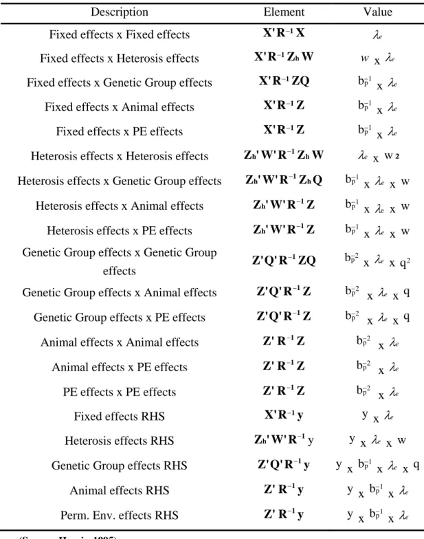
b− [Harris, 1995]. Table 3 gives the contributions for solving the MME by iteration on data methods.
Table 3: Contributions for solving the MME by iteration on data methods.
Description Element Value
Fixed effects x Fixed effects X'R−1X
e
λ
Fixed effects x Heterosis effects X'R−1ZhW w x λe Fixed effects x Genetic Group effects X'R−1ZQ bp−1 x λe
Fixed effects x Animal effects X'R−1Z bp−1
x λe Fixed effects x PE effects X'R−1Z 1
p b− x λe Heterosis effects x Heterosis effects Zh'W'R−1ZhW λe x w² Heterosis effects x Genetic Group effects Zh'W'R−1ZhQ bp−1
x λe x w Heterosis effects x Animal effects Zh'W'R−1Z bp−1
x λe x w
Heterosis effects x PE effects Z'W'R 1Z
h − bp−1 x λe x w Genetic Group effects x Genetic Group
effects Z'Q'R ZQ
1
− 2
p
b− x λe x q 2
Genetic Group effects x Animal effects Z'Q'R−1Z 2 p
b− x λe x q Genetic Group effects x PE effects Z'Q'R−1Z 2
p
b− x λe x q Animal effects x Animal effects Z'R−1Z 2
p b− x λe Animal effects x PE effects Z'R−1Z 2
p b− x λe PE effects x PE effects Z'R−1Z 2 p b− x λe Fixed effects RHS X'R−1y y x λe Heterosis effects RHS Zh'W'R−1y y x λe x w Genetic Group effects RHS Z'Q'R−1y y x bp−1
x λe x q Animal effects RHS Z'R−1y
y x 1 p b− x λe Perm. Env. effects RHS Z'R−1y
y x 1 p b− x λe (Source: Harris, 1995)
4.2. Genetic evaluation system of live weight
The animal model used for live weight is the same model as the one used for production traits: it is a repeated records, single trait, additive genetic and simple repeatability model.
The statistical model is the same as for production except the effects for induction and period of calving are replaced with an effect for stage of lactation when weighed nested within age [Harris, 1995; Harris et al., 1996].
4.3. Genetic evaluation systems of the linear type traits and survival
The models are single record, single trait, additive genetic models according to Henderson [1988].
The statistical model for analysis of a cow with linear type scores includes effects for herd-season contemporary group, stage of lactation class when scored and age at first calving class in months nested within breed, heterosis, genetic group, random animal genetic merit and the random residual [Harris, 1995; Harris et al., 1996].
The statistical model for survival is the same as for linear type except there is no effects for stage of lactation or age at calving. The herd-season-age for survival is assigned as the herd-season-age immediately prior to the survival record [Harris, 1995; Harris et al., 1996].
4.4. Use of genetic groups and relationships
A grouping strategy developed by Westell et al. [1988] in which a genetic group for each animal is derived from the genetic group effect of the animal’s ancestors is used. For each animal with unknown ancestors, phantom parents without records are created and are assigned to appropriate genetic groups; the relationship matrix is augmented to include those. The genetic group effects represent the average genetic merit of the phantom animals selected to be parents to their descendants that do have records available. Phantom parents are assumed to be unrelated to one another [Harris et al., 1996]. More information about the transformation and the absorption of the augmented MME are available in Quaas and Pollack [1981], Westell et al. [1988], and Wiggans et al. [1988].
In a multibreed animal model genetic groups are assigned by breed; in the case of an animal who is ¾ breed A and ¼ breed B with a known pure breed parent, the phantom parent would be a ½ A x ½ B crossbred. Therefore, the animal would be assigned to both the genetic groups for A and B with values of ½ for the unknown parent. More details about computation rules can be found in Harris [1995].
Thus, genetic groups are assigned by sex (male or female missing parent), birth year, country of origin and breed (eight classes). So, when both parents are known there is no need to assign genetic groups; genetic groups must be assigned if one or more parents are unknown. Genetic groups are assigned in 5 years intervals after 1960 to 1980 then yearly with the first group being prior to 1960 [Harris, 1995].
After merging small groups across years and across countries, in which there is a insufficient number of animals assigned, there are 125 genetic groups. There is no clustering across breed or sex [INTERBULL, 2004].