Inspection of local deformations using 3D scans

Inspection of local deformations using 3D scans

Thèse

Sarah Ali

Doctorat en génie électrique

Philosophiae Doctor (Ph.D.)

Québec, Canada

iii

R

ÉSUMÉ

De nombreuses recherches sont conduites dans le domaine de la vision 3D pour effectuer la comparaison entre les modèles 3D d’objets et d’êtres humains. En fait la comparaison des modèles 3D est apparentée à la récupération des modèles appartenant à une grande base de données et elle comprend les procédures suivantes : la reconnaissance des objets, leur classification en catégories ou groupes selon leur type et enfin la comparaison des objets d’un même groupe afin d’identifier certains aspects de conformité ou de variabilité de la forme. L’alignement des modèles 3D entiers permet de comparer ces modèles et de détecter la déformation locale.

Il existe deux sortes de déformations des objets: la première déformation affecte principalement la position des parties de l’objet ou bien l’objet tout entier dans le cas d’articulation, de fléchissement ou de contraction sans aucune altération du volume. La deuxième déformation résulte d’un changement de volume de l’objet dû à une variation de masse. D’autres cas plus compliqués existent quand le changement de la forme comporte les deux sortes de déformations à la fois.

Dans ce projet on présente une "méthode d’inspection" basée sur un alignement exact des parties rigides des modèles 3D qui ont subi une déformation locale. Ici la déformation locale implique le changement de quelques parties des modèles plutôt qu’une déformation globale. On présente une approche capable de détecter la région qui a subi un changement pour un objet qui s’est déformé avec le temps. Cette approche explore deux types de transformations intéressants : la transformation altérant le volume d’un corps suite à une inflation ou une déflation d’une ou de plusieurs parties de l’objet et la transformation conservant le volume résultant d’un cintrage, d’une torsion, d’une rotation ou de l’écartement d’une ou de plusieurs parties d’un objet. En général, les parties internes sont les parties au voisinage du centre de gravité, tandis que les parties externes sont situées à l’extrémité d’un corps.

Différents cas de déformation sur des objets synthétiques et des objets réels ont été étudiés afin de détecter les défauts pouvant se présenter lors leur fabrication pour vérifier et contrôler la qualité de cette construction. On a aussi testé notre approche de comparaison sur des parties du corps humain entre autres pour la détection et le dimensionnement d’une lésion (tumeur) visible en surface. Notre méthodologie réussit à détecter des déformations locales avec une précision meilleure sinon comparable à d’autres méthodes d’inspection industrielle.

v

A

BSTRACT

In 3D vision several studies have been conducted to perform the comparison of 3D objects or human models. In fact the comparison of 3D models is sometimes related to the retrieval of models belonging to a large database, and it includes the following procedures: the recognition of objects, their classification in categories or groups according to their types and finally the comparison of the models in the same group in order to identify certain aspects of resemblance or variability in their shapes. The alignment of entire 3D models also enables their comparison for the detection of possible local deformations.

There are two sorts of deformation of models: the first mainly affects the position of parts of the object or the whole object in cases such as the articulation, the stretching or the contraction of parts without altering the volume of the object. The second type of deformation results from a change in volume due to mass variation. Other more complicated cases occur when the change in form includes both kinds of deformation at the same time.

In this project we propose an “inspection method” based on an exact registration technique of the rigid parts of the deformable models that have undergone local deformations. When the deformation is local, it means that there is a change of some parts of the model rather than a global deformation of the whole object. We propose an approach that is able to detect the region of deformation. This approach exploits two kinds of local deformations: non-volume conservative transformations caused by either the inflation or the deflation of models’ parts and volume conservative transformations caused by bending, twisting, rotating or displacement of either internal or external parts of the model. In general, the internal parts are the middle parts of an object, while the external parts are the parts at the extremities or the end parts.

We have experimented on different cases of deformations on man-made objects and mechanical parts for industrial inspection of possible artifacts and defects, and for quality control purposes as well. We have also applied our comparison method on parts of the human body. Examples relevant to medical applications are the detection and inspection of a lesion which are also tested in this work. Our algorithm is not only successful for detecting local change but it also achieves high accuracy comparable to other well-known industrial inspection technique.

vii

T

ABLE OF

C

ONTENTS

Résumé ... iii

Abstract ... v

Table of Contents ... vii

List of Figures ... xi

List of symbols ...xiii

Acknowledgments ... xix

Chapter 1. Introduction... 1

1.1 Comparison of deformable models ... 1

1.2 3D vision- based inspection methods for local comparison ... 2

1.3 Motivation ... 4

1.4 The problem and the solution ... 5

1.4.1 Challenges ... 6

1.4.2 Description of the solution of the problem ... 8

1.4.3 Expected outcome ... 8

1.4.4 Thesis outline ... 10

Chapter 2. Global comparison methods ... 11

2.1 Global features ... 11

2.1.1 Spectral embedding ... 13

2.2 Local descriptors ... 15

2.2.1 Curvature maps ... 15

2.2.2 Histogram of local features ... 16

2.2.3 Bag-Of-Features ... 17

2.3 Spatial maps ... 21

2.4Combining topological and geometric features ... 23

2.5 Experimental results ... 25

Chapter3. Literature review on segmentation, partial matching, alignment of 3D models and distance computation between 3D models. ... 31

3.2 Partial matching ... 33

3.2.1 Partial Matching using the Bag-of-Features approach ... 33

3.2.1 Salient geometric features for partial shape matching and similarity ... 35

3.2 Alignment of 3D models ... 36

3.3.1 Rigid point sets registration methods ... 37

3.3.2 Non-rigid registration methods ... 38

3.4 Computation of the shortest distances between two 3D surfaces ... 40

Chapter 4. Description of the local comparison approach for simple models ... 43

4.1 Alignment of models with volume change ... 44

4.2 Alignment of models with volume conservation ... 46

4.3 Computation of the shortest distances between the models after alignment ... 49

4.4 Experiments ... 51

4.4.1 Effectiveness of the method ... 52

4.4.2 Accuracy of the method for the measurement of change ... 54

Chapter 5. Local comparison for models with complex geometry ... 57

5.1 Preprocessing of the data ... 58

5.2 Segmentation of the deformed model into critical parts ... 59

5.3 Partial matching ... 63

5.3.1 Part-to-whole-matching for the detection of rigid parts ... 65

5.3.2 Discussion on the number of clusters ... 67

5.4 Detecting and displaying the deformation ... 69

5.4.1 Partial alignment ... 69

5.4.2 Global alignment ... 70

5.4.3 Distance computation and estimation of the degree of deformation ... 70

5.5 Experimental results ... 72

5.6 Quantitative Evaluation of the accuracy and the repeatability of the method ... 79

5.7 Comparison with other methods ... 89

5.8 Another method to compute the shortest distance between a point cloud and a surface mesh ... 92

Chapter 6. Additional measurement and comparison of deformed and non-deformed objects ... 97

6.1 Area and volume of a 3D mesh ... 97

ix

6.2 Computing the geodesic distances between 2 points ... 100

Chapter 7. Conclusion ... 103 7.1 Overall Contributions ... 103 7.2 Pertinent Applications ... 105 7.3 Future work ... 106 Appendix ... 107 BIBLIOGRAPHY ... 108

xi

L

IST OF

F

IGURES

Fig. 1 Inspection of 3D models using the 3D scanner software Reshaper1 _{... 3}

Fig. 2 The alignment of the original to the deformed model ... 7

Fig. 3 3D model of a wrench before deformation ... 9

Fig. 4 3D model of an apple slicer before deformation ... 9

Fig. 5 Shape distributions ... 13

Fig. 6 Articulated shapes from the McGill database ... 14

Fig. 7 SISI descriptors... 17

Fig. 8 Bag-Of-Features for spin image descriptors ... 18

Fig. 9 The Bag-Of-Features of local SIFT descriptors ... 20

Fig. 10 Computing feature maps ... 23

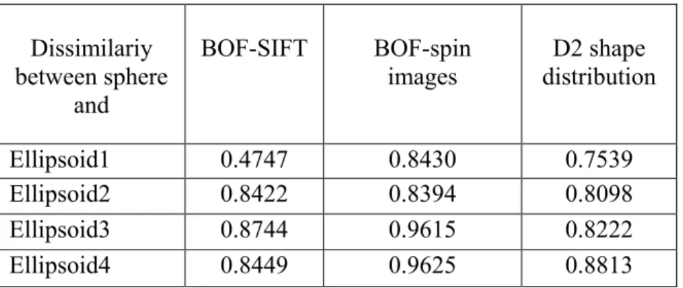
Fig. 11 The sphere and the elongated ellipsoids ... 25

Fig. 12 The curves of dissimilarity ratios ... 26

Fig. 13 Matching parts of the deformed models of flowers with holes ... 28

Fig. 14 Matching parts of the deformed models of flowers ... 29

Fig. 15 Bag-Of-Features for spin images descriptors ... 35

Fig. 16 The diagram of local comparison of simple models ... 44

Fig. 17 Alignment using ICP alone ... 47

Fig. 18 K-means segmentation of a CAD model into two parts ... 48

Fig. 19 Computation of the shortest distances ... 51

Fig. 20 The models of the cube before alignment ... 53

Fig. 21 The color map of the computed distances in mm after alignment ... 53

Fig. 22 Experiments performed on a second deformable model ... 54

Fig. 23 Colormap of the distances in mm after alignment ... 55

Fig. 24 Diagram of the proposed methodology ... 58

Fig. 25 3D-NCuts segmentation results for 6 models ... 62

Fig. 26 Pseudo code 1- Separating clusters from a segmented mesh ... 62

Fig. 27 The segmentation of a mechanical parts into two segments with 3D-Ncuts ... 63

Fig. 28 Spin images... 64

Fig. 29 Deformation of the wrench ... 66

Fig. 30 Part-by Part matching of the segments ... 68

Fig. 31 Rigid part detection with our approach ... 70

Fig. 32 The alignment of the deformed model ... 70

Fig. 33 Orientation of the normals of the point cloud of a part of a kitchen environment. ... 72

Fig. 34 Deformation cases caused by the inflation or the deflation of the critical parts of the objects ... 73

Fig. 35 Deformation cases caused by the displacement ... 74

Fig. 37 The 3D scans of an apple cutter ... 76

Fig. 38 Unsuccessful aligment of the handle of the deformed model ... 77

Fig. 39 The hand model of the PSB benshmark before and after deformation ... 78

Fig. 40 The dummy model before deformation. ... 78

Fig. 41 The car door model before deformation.. ... 79

Fig. 42 Planar objects ... 79

Fig. 43 Block models ... 80

Fig. 44 Planar objects ... 80

Fig. 45 Inspection of the CAD models using Polyworks... 81

Fig. 46 The color map of the wrench and the apple cutter ... 86

Fig. 47 The translation stage ESP600 controller. ... 87

Fig. 48 The curve of computed distances of 6 different experiments for the distance 5.9 mm. ... 87

Fig. 49 The curve of computed distances of 6 different experiments for the distance 3.02 mm. . 87

Fig. 50 The curve of computed distances of 6 different experiments for the distance 2.77 mm. . 88

Fig. 51 The curve of errors of 6 different experiments for the distance 5.9 mm. ... 88

Fig. 52 The curve of errors of 6 different experiments for the distance 3.02 mm. ... 88

Fig. 53 The curve of errors of 6 different experiments for the distance 2.77 mm. ... 88

Fig. 54 CPD non rigid alignment [89] (left) versus our registration method (right). ... 91

Fig. 55 Registration of the two different poses of the cactus and elephant models ... 92

Fig. 56 Detecting the deformation using the method in section 6.3 ... 93

Fig. 57 Distance computation by projecting a vertex in P onto the surface of Q. ... 94

Fig. 58 A tetrahedron



Fig. 59 Computing the geodesic distance between two selected points. ... 101

xiii

L

IST OF SYMBOLS

P /D point cloud 2 without the region of deformation

1 P Point cloud 1 2 P Point cloud 2 D Region of deformation 2 D Shape distribution M G Graph V Vertices M E Connected edge j i A Gaussian matrix



d



N

v)

S(u, Surface penetration

A Model B Model i

P

W

R

L

n

)

,

,

(

x

y

z

F

dist Distance V Vertices

xv F Faces W Similarity matrix i

C

xvii

xix

A

CKNOWLEDGMENTS

I would like to thank my advisor Denis Laurendeau for his constant help and encouragement during this project. This person believed in me and never hesitated to listen to me. He gave me all the guidance whenever I needed. For me he is more than an advisor. He is my scientific father. Also my appreciation and gratitude go to Denis Ouellet, Chen Xu and all my dear colleagues and friends in the Computer Vision and System Laboratory at Laval University: Zahra Toony, Van-Toan Cao, Trung-Thien Tran, Van-Tung Nguyen, Dominique Beaulieu, Guillaume Villeneuve, Somayeh Hesabi and Wael Ben Larbi for their support and encouragement, wishing them always the best in their future endeavors. I will also never forget Annette Schwerdtfeger for her pertinent comments and her corrections made in all my manuscripts. This work was supported by the NSERC/Creaform Industrial Research Chair on 3D scanning.

I am indebted to family for their support and understanding: My mother Amal, My father Ali and my siblings Ronda, Suzette and Wissam. I will not forget my uncles: Fred, Juliano, Gus and my aunt Sonia for their support and encouragement. I dedicate this thesis to them with all my love and affection.

1

C

HAPTER

1.

I

NTRODUCTION

1.1 Comparison of deformable models

In computer vision many research studies have been conducted in order to perform the matching and the comparison of 3D models of objects. The main goal of matching is to group the models into different categories according to their similarity in order to allow their retrieval for recognition purposes and for further usages. So, in most cases, the comparison is run on a large dataset containing various models whether they belong to the same type of object or not and generally having similar or different shapes and poses. The objects’ characteristics and nature are important factors to be taken into consideration before performing the comparison process. We distinguish between two main categories of objects: rigid objects and deformable objects whose treatment and handling differ in the modeling as well as in the comparison phases. In our work, we focus on the comparison of objects with a deformed instance of themselves, which means we deal with objects whose shapes may vary with time. The deformation or variation in shape has different aspects depending on the type of object. It could be a change in the posture of an articulated or bendable model, or it could result from a variation (loss or gain) in the repartition of mass leading to a change in the volume and thus in the shape of the object; even more complex situations occur when both cases are combined together.

The process of comparison generally relies on the extraction of features or descriptors from both models. In general, the extracted features can be based on the topology, the geometry of the models or both. A comparison based on topology gives information about the skeletal structure of the model. Topological features can be used in the retrieval of objects that represent the same models but in different positions. Methods based on geometry usually rely on descriptors and features that allow a high discrimination between shapes. Comparison also might be done using alignment techniques that can detect deformations of 3D models.

Most of the comparison methods try to meet several criteria such as invariance to: (1) similarity transformations of the scans (2) shape representations, (3) geometrical and topological noise, and (4) articulation or global deformation. Such methods might also use shape features that are invariant to geometrical transformations, pose normalization or a combination of both to achieve their goals. In this work, a survey on the main approaches used for retrieving 3D models based on geometric and topological features is presented in chapter 2 in addition to experimental comparison for some of these methods to compare global 3D models and partially match them as well.

1.2 3D vision based inspection methods for local comparison

Despite the fact that the features described above enable good comparison among the deformable models, they are generally more convenient in retrieving models from large datasets and classifying them into categories by providing a global percentage of similarity of the models than for comparing shapes. Here the similarity is defined by how much the different models look alike or fall in their own category in the large database of models. For example, in a large database containing hundreds of different deformable models of horses, cats, trees and planes, the similarity ratio serves to identify the horses in one category, the planes in another category, etc. However, these methods of comparison cannot localize the change or describe the deformation undergone by the models. Our objective is to provide a 3D vision-based inspection technique for comparing locally deformable models which identifies the deformation and gives accurate measures of the local change.

Recent advances in computer vision have shown that the inspection of 3D objects is crucial and is extremely relevant in many fields such as: architecture and cultural heritage; industry and quality control; digital terrain models and surveying; medical and dental applications. Generally, the inspection of 3D models involves the task of "comparing" two objects. It can also be called: CAD

compare, part-to-CAD analysis or surface control. The process of 3D inspection can be

summarized as follows1 _{(see Fig. 1):}

 Reading the reference model (CAD model) in the inspection software.

 Measuring accurate 3D coordinates of an object with a Coordinate Measuring Machine (CMM) or a 3D scanner and loading the scan in the software.

 Aligning or registering the scanned model to the CAD model.

 Performing distance computation and color coding of measured distances between the scan and the CAD model.

 Adding flags and labels if needed on the scanned model to enable the comparison.  Finally producing a 3D color mapping inspection report.

To highlight the importance of local comparison of deformable objects, we discuss some relevant examples. In medical applications, observing the change of the shape of the human body is important in identifying treatments and relevant solutions for some problems. For instance in the case of obesity, comparing the shape and identifying the parts of the body that have changed most is an important issue to determine how effective a diet is on the human body with respect to weight loss. In addition, comparing the shape of an organ or a body part is important in the detection and

3

the location of a tumor or a bending such as scoliosis, and it helps in the prescription of the medication dosages in such cases as well. Shape comparison over time may also be useful for assessing the level of healing of an external wound. Our approach was applied to detect and measure lesions on human body parts and it led to good and reliable results.

CAD model Scanned model

inspection

Fig. 1 Inspection of 3D models using the 3D scanner software Reshaper (taken from

http://www.3dreshaper.com/en1/En_Inspection2.htm).

Another example borrowed from the industrial context is designing and restoring heavy machines; it is relevant to compare the parts of the machine that were subjected to deformation, locate where this deformation occurred and estimate the extent of deformation. This also applies to the comparison of manufactured parts that may change in shape when installed or while being used in a system or machine. All of the above applications are very complex problems when it comes to comparing shapes. Furthermore, local comparison of deformable models is relevant in the industrial inspection of mechanical parts and manufactured objects to detect possible artifacts and defects after the fabrication, and for quality control purposes as well. We have experimented on different cases of deformations on man-made objects and mechanical parts for industrial inspection of possible artifacts and defects. Our algorithm is not only successful in detecting local

change but it also achieves high accuracy results comparable to other well-known industrial inspection techniques.

As mentioned before, our aim is to perform a pairwise comparison of deformable 3D objects leading to results with sufficiently high precision. What is meant by comparing deformable 3D objects is more specifically to consider an object and scan its 3D model M₁ at a certain time t1,

then take the same object but with a given deformation of its shape, build its 3D model M₂ again

at a time t₂ and compare the shape of the 3D models M1 and M2. The experiments are offline,

meaning that the comparison is not performed in real-time, and the main challenge is to reach the best comparison accuracy. The purpose is to develop a system able to compute the amount of change between two objects and determine where this change is located on the subparts of the models by estimating its importance and, as much as possible, the direction and absolute amount of change between the shape of an object prior change and its shape after change. Thus the comparison is pairwise (i.e. an object with itself) and not between many objects in a large database where the objects are of the same type or of different types.

1.3 Motivation

The comparison methods of deformable models described in section 1.1 are used for retrieving models which belong to the same category of a query model based on the similarity of the features extracted from each model. In such approaches, a similarity measure must be defined, so that a pair of models can be compared. The similarity is a percentage of resemblance between the features of this pair, but it cannot be taken as an absolute measurement of the change between them because this percentage might change from one approach to another. In addition, this percentage cannot identify where the change has occurred. It is simply a criterion to rank the models which are more likely to be similar to the query. Therefore, the comparison becomes insufficient because it is impossible to localise the deformation and to estimate its level with respect to the original non-deformed object which created an initiative to investigate inspection methods of 3D models. Moreover, registration techniques (whether rigid or non-rigid) cannot guarantee an exact overlap of the rigid parts of all sorts of 3D deformable models in the real life. Meaning that a certain approach of registration is not guaranteed to be successful for all cases of deformations and might unexpectedly fail for certain geometric shapes of 3D models. For instance some methods are more suited for certain kinds of deformations such as articulations of articulated 3D models [91, 92, 93, 94].

When we have used inspection software for comparing 3D models, we encountered many challenges. First, the majority of inspection software performs a local comparison only between the scanned model (whether it is a point cloud or a mesh of the model) and its original CAD model. Thus the inspection requires the existence of the CAD model, which is not the case in our project

5

since we need to investigate real scanned models of deformable objects, which do not necessarily have their corresponding CAD models. Furthermore, all inspection software require that both models (the scan and the CAD) be very similar to each other or to differ slightly in distances after their alignment, which is also not the case in our project since we deal with some cases involving a 60% change in size caused by deformations (see the models in Fig 41, 42 and 43). Other models might have more than one local deformation (models in Fig 29, 35-1, 35-2, 37 and 40) which is a challenge we address in this thesis.

Another problem we encountered using such inspection software is that the alignment of the real scanned deformable models cannot be done automatically, since the overlap is not significant. The existence of the deformation causes the automated alignment to fail most of the time. Now, to solve this problem, an initial alignment position has to be set manually by selecting a set of common correspondent points in the same region of both mesh models. This will also affect the results of the inspection accuracy since there is no guarantee that the alignment is “ideal” between the original and the deformed model. By ideal, we mean that the alignment should allow the non deformed parts to be as close as possible to each other.

To approach this problem we used an idea which might seem very trivial but which is based on a relevant observation on which our whole work is based. This observation is indeed aligning the non-deformed parts of an object as accurately as possible to the same parts prior change. For instance, first, we can scan the original object using a 3D sensor then we install external markers on the object and save their positions. Afterwards, we deform a region of the object without changing the position of the object, we erase manually the region of deformation but we save the positions of the markers, and then we scan the deformed objectagain focusing on the missing part which will definitively include the region of deformation. This will insure a perfect alignment between the original and the deformed model, since there will be a significant overlap between rigid parts of both models which are the parts that did not deform or that remained intact because the saved markers gave us a lot of information on the non-deformed parts. Certainly this idea cannot be applied in practice since we cannot deform an object without changing its position and we cannot always save the position of markers on the region containing the non-deformed parts. Consequently, we need to develop an automated method that guarantees a good alignment between the two scanned models and also provides accurate measurements of the distances between the aligned models. This approach is implemented in this thesis.

1.4 The problem and the solution

In this section we introduce the main challenges of this work, next we describe the solutions finally we give the expected outcomes.

1.4.1 Challenges

The main problems we have addressed in the research are:

I. To perform the alignment of the 3D models of the object before and after the deformation. The object undergoes two kinds of transformation. First a non-rigid transformation resulting from an unknown change in a certain region of the object. Second a rigid transformation caused by the change of the position of the deformed object in the reference frame of the original object before the deformation. This problem cannot be entirely solved using non rigid alignment methods. Let P₁ be the

point cloud of the original model M₁of the object before deformation, P2 the point

cloudof the deformed model of the object after the deformation, and let D be the region of deformation ofP₂. After the non-rigid alignment, P2 is deformed to be as

close as possible toP₁. Therefore, the region of deformation D might disappear

because of the alignment so it will be impossible to compute the change or estimate its level. Similarly, no matter what the objective optimization function used, rigid alignment alone cannot solve the problem since the region of deformation D affects the convergence of the rigid parts (non-deformed parts) of P2 toward the rigid parts of P1.It is thus crucial to eliminate the region D from P₂for the alignment, since it is caused by a non-rigid transformation and then perform a rigid alignment between P₁

and P₂ /D. The final result of alignment will be a perfect overlap between the rigid parts of both models before and after the deformation while the parts containing the region of deformation will remain observable and distinct from the original model M₁

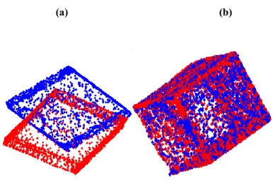
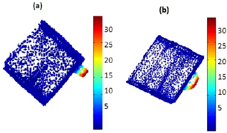
Fig. 2 shows an example of the desired alignment of two models of a mechanical part after deforming its external parts (the end parts) by displacement. P₁ is the point cloud (in red) of the original model and P2 is the point cloud (in blue) of the deformed models. We can see after the alignment that rigid parts (the flat parts at the bottom) are overlapping while the displaced parts (the external deformed parts) are observable and distinct from the external parts of the model before deformation.

II. Another challenge is to create a shape representation to model the shape of the object (for example polygonal meshes, point sets, etc.) and extract the features from this representation in order to perform the comparison of the models.

III. To extract the region that contains the local change or deformation of the mesh model, and represent it by a set of vertices (point clouds) and faces (the possible connection between these points), and to compare this region with the original model using the extracted features.

IV. To identify the rigid parts and the deformed parts in the 3D model of the deformed object.

7

V. To compute the absolute change between both models before and after deformation.

Rigid Parts Deformed parts

Fig. 2 The alignment of the original to the deformed model. The rigid parts are overlapping while the deformed parts

are observable.

On the other hand, two main challenges were not addressed in this thesis:

I. The segmentation of 3D models into critical parts. In this work, a clustering technique called the 3D-NCuts that is run on triangular meshes resulting from the scans [43] was applied in order to segment the model into critical parts. Critical parts are important parts an object could be segmented to. Among these parts are those parts that remained intact with respect to the original model (rigid parts) and other parts that have undergone a significant modification (non-rigid parts) due to either non volume conservation transformations (inflation or deflation of the parts) or volume conservation transformations (bending or twisting of inner parts, spacing of outer parts).

II. The comparison of full human bodies is not addressed in this work since the alignment of 3D models of human bodies differs from the alignment of scanned free-form objects. In practice, in the alignment of full human bodies, most of the methods rely on a set of landmarks that are placed manually on certain parts of the body (such as head, torso, arms and legs) before scanning. These methods might sometimesbe inaccurate because it is hard to correctly fix the location of these landmarks on the human body which is subject to deformation due to change in shape (gain or loss in weight) or in postures due to body articulations. In addition, these landmarks should be identified manually on the scans. This process is time consuming and error prone. Other methods for aligning human models rely on fitting a low-resolution artistically created template mesh model to high-resolution laser

scans of human bodies. These methods also rely on initial landmarks and provide good results only if the body poses are fairly similar to each other [88].

1.4.2 Description of the solution of the problem

In this work, a 3D inspection approach so as to locally compare deformable 3D models is presented using the 3D meshes and point clouds of the objects. Two types of deformation are discussed (see Fig. 16). The first is volume change which is caused by either an increase or a decrease of the body volume. In the second type of deformation, the volume of the model is not altered but the change in shape results from either an articulation or a bending of parts of the object. For each case of deformation, we consider both original and deformed 3D models of man-made objects, mechanical models and some parts of the human body. Based on these models, a set of pre-processing steps such as smoothing, and simplification techniques are used to prepare the final 3D models for comparison. After pre-processing, the deformed 3D model is segmented into critical parts (the number of critical parts is chosen by the user). Among the critical parts are rigid parts (parts that are intact and were not affected by the deformation) and non-rigid parts (parts that have undergone a deformation such as bending, spacing, inflation or deflation). Following segmentation, a partial matching technique is applied to the segmented critical parts and the original non-deformed model in order to separate the rigid parts from non-rigid ones. The rigid parts are aligned to the original model which enables the computation of the transformation (rotation and translation) that is later used to globally align the original model to the deformed one. Finally, to detect the deformation of the object, the approximate shortest distances from the deformed model to the surface mesh of the aligned original model are computed and a color map of these distances is produced. This distance color map is used to display the location and the level of deformation of the object which is useful for inspection and quality control purposes.

1.4.3 Expected outcome

The objective of this project is to detect the deformation in a model and to estimate its level. So the output of the result would be to display the region of deformation on the 3D model of the deformed object and to show the level of change with respect to the original parts of the model. We began exploiting simple shapes of models such as cubes, spheres and planes, in which we created deformation that can be measured easily. We also constructed the CAD models of these objects before and after deformation. Then we compared these models using the Polyworks inspection software to be able to measure the maximal level of deformation. Our strategy of automatic inspection in order to locally compare these models gave comparable results to those obtained by the inspection software. The accuracy of the results was good and repeatable. Then we extended the approach to compare more complex models such as industrial objects and

9

and twisting; and displacement of certain parts of these models. The 3D mesh models of the manufactured and mechanical objects were acquired using two Creaform 3D sensors: the Go!Scan2 _{and the Metrascan}3_{. The Metrascan, which enables high precision scans, was used} mostly to scan models with sharp edges and thin parts such as the wrench (Fig 3) and the apple slicer (Fig 4), which are examples of mechanical models having fine details. We also tested our approach on large industrial parts as well and the results were satisfying as demonstrated in Sec. 4.4, 5.5 and chapter VI.

(a) (b)

Fig. 3 (a) 3D model of a wrench before deformation. (b) Detecting the deformation of the bent parts of the wrench

model using a color map of measured distances in mm.

(a) (b)

Fig. 4(a) 3D model of an apple slicer before deformation. (b) Detecting the deformation of the twisted parts of the apple cutter model using a color map of measured distances in mm.

2 _{http://www.goscan3d.com/en}

Examples relevant to medical applications are the detection and inspection of a lesion on human body parts such as the hands and the torso were also tested and the results were convincing. Our approach could be relevant to other medical applications such as obesity monitoring in order to compare the shape and identify the parts of the body that have changed. This application has been identified as having potential for future work.

1.4.4 Thesis outline

This thesis introduces a new 3D vision-based approach to inspect the deformation by comparing 3D models locally. In the second chapter we discuss and analyse the different methods that compare deformable models globally. Such methods are mainly used for the retrieval of deformable models. We also present experimental results on some of these global comparison methods performed on different 3D models. These results show the limitations of global comparison methods and stress the need for more effective approaches.

In the third chapter we present a brief review on computer vision techniques that are relevant to our work such as the segmentation, the partial matching and the alignment of 3D models. Finally we discuss some methods to compute the shortest distances between two 3D surfaces of models. In the fourth chapter we present a local comparison approach that could be used to compare simple shapes (such as spheres, ellipsoids and cubes) of deformable models that undergo two sorts of deformations: transformations with volume conservation, and transformations with volume variation.

In the fifth chapter we describe our 3D vision-based inspection approach so as to locally comparing complex and free-form shapes of 3D deformable models. We begin with the segmentation of the deformed model into critical parts. Then we propose a part-to-whole matching technique used to compare these critical parts to the original model in order to determine the rigid parts of the deformed model. Afterwards the alignment of both models before and after deformation is performed. Finally an efficient technique to compute the shortest distances between the surfaces of the aligned 3D models is proposed. In addition to the theoretical concepts of the proposed 3D vision-based inspection approach, we also present the experimental setup used for experiments and we analyse of the results of our local comparison approach performed on complex and free-form shaped of deformable models. In addition we suggest another method to compute the shortest distances between 3D models after alignment and we compare with 3 different methods of alignment of the deformable 3D models.

In the sixth chapter we perform additional relevant comparative measurements on 3D models, such as measuring the area and volume of 3D meshes and computing geodesic distances.

Finally we summarize the overall contributions of this thesis. We give potential applications that could be investigated as future work.

11

CHAPTER

2.

G

LOBAL COMPARISON METHODS

This chapter is a literature review of methods [99] for comparing objects for the purpose of recognition. They all use some kind of descriptor of the shape, which is them compared to a database of previously computed descriptors. It is assumed that the object is similar, but can be very deformed compared to its match in the database. The goal from such methods is not to measure the deformation (its localization and magnitude), accurately but simply to find a match. It is very important to remind the reader that our main objective is to do a “deformation

qualification” rather than a “recognition” of an object.

In general, global comparison methods of 3D models can be based on their topology, their geometry or both. A comparison based on topology, which refers to “the anatomical structure of a specific area or body part”, gives information about the skeletal structure of the model.

Topological features can be used in the retrieval of objects that represent the same models but in different positions. Methods based on topology are generally computationally costly [1].

However, methods based on geometry are used more frequently since they usually rely on descriptors and features that allow a high discrimination between shapes.

Comparison methods which use geometric features are classified into three major categories according to the type of shape feature [2]: (1) global features, (2) histograms of local features, and (3) spatial maps. Global features describe the shape with moments, aspect ratio, or volume-to-surface ratio. Histograms of local shape features consist of bins, each bin storing the

probability of occurrence of a feature. Generally, histograms are invariant to rotation, reflection, and uniform scaling of objects; they are used to represent various features such as angles, distances, areas, volumes and curvatures. Examples of histograms such as spin images [3] and shape contexts [4], which represent the relative positions of the data points, have also been used for matching and recognition tasks. Finally, spatial maps represent the spatial information of an object’s features meaning that they usually store information about the location of the features in an object. For example, distance maps and surface penetration approaches introduced by [2] are spatial maps able to describe the geometry of the object’s shape, the topology and concavity of the entire object.

2.1 Global features

Over the last few years, the number of methods that involve comparing and retrieving 3D models has increased significantly. These methods mainly use geometric descriptors extracted from 3D shape representations (e.g. 3D polygonal meshes and point clouds), represent and compress these features in a certain manner to enable their comparison and then to compare the different models in large databases.

Methods that use global descriptors for retrieving 3D models have gained considerable interest over the last few years. The most popular methods in the retrieval of 3D models involve the use of the following global descriptors: the D1 descriptor [5], the D2 descriptor [6], the spherical harmonic descriptor SHD [7], the 3D wavelet descriptor [8], the skeleton descriptor [9], the Reeb graph descriptor [10], the depth buffer images, silhouettes, and ray-extents DESIRE [11], etc. For example, the D2 shape distribution of [6] represents the distribution of Euclidian distances between pairs of randomly sampled points. Therefore, 3D models are transformed into parameterized functions which facilitate their comparison using an appropriate similarity measure (see Fig. 5).The main advantage of this approach is its simplicity because the shape matching problem is reduced to the following tasks: random sampling, normalization of models, and comparison of their probability distributions. This is to be compared to methods that require the reconstruction of manifold surfaces from degenerate 3D data, the registration of pose transformations, the matching of features and the fitting of high-level models. Despite the fact that the D shape distribution 2 enables good results in retrieving rigid objects, itsometimes fails in comparing complex shapes because some features might be missing in the random sampling.

Another interesting example of a global shape descriptor is spectral embedding (see section 2.1.1 below). The spectral approach derived from the graph theory of matching can be applied in 3D geometry for purposes such as finding point correspondence, segmenting and compressing 3D meshes and retrieving articulated 3D models [12]. The global geometric descriptors used in the spectral approach are invariant to shape articulation and bending where a spectral embedding representation of the 3D shape is proposed by only considering the first knormalised eigenvectors of the affinity matrix A of the graph G _M (V,E_M) of a specific mesh M having V as the set of vertices and E_M as their connecting edges. The eigenvectors are scaled by the square root of their appropriate eigenvalues. These eigenvalues can be used as effective descriptors which enables the retrieval of articulated 3D models of the McGill University benchmark database (MSB) [21].

13

Fig. 5Shape distributions. Shape distributions facilitate shape matching because they represent 3D models as

functions with a common parameterization. Taken from [6].

2.1.1 Spectral embedding

In the spectral approach, the input models are given by 3D meshes containing hundreds of thousands of faces [12]. In order to facilitate feature extraction, the resolution of the meshes is reduced using mesh simplification techniques. Next the affinity matrix A of the graph

) ,

( _M

M V E

G  of a specific mesh M having V as the set of vertices and E_M as their connecting edges is constructed. The affinity matrix is of size n , where n is the number of vertices of the n

mesh M. In the affinity matrix A the entry d_ijcorresponds to the minimum geodesic distance between the _{i and}th _{j vertices of the mesh. The geodesic distances give the smallest curve} th

distances between any 2 points of the 3D mesh model. Unlike the Euclidian distances, the geodesic distances are invariant to certain shape bending. Therefore, their use is shown to be relevant especially when retrieving deformable 3D models that undergo shape articulation and bending. After computing the affinity matrix of the geodesic distances, it is normalized using a Gaussian distribution, and it is given by the Gaussian equation:

) 2 / exp( 2 _2 j i j i d A   (1),

Where  is defined by the Gaussian width and it is set to  max(i,j){dij}. In the next step, the spectral embedding (i.e. the eigenvalues and eigenvectors) are computed. It is sufficient to consider only the first k largest eigenvalues and their corresponding eigenvectors (generally the eigenvectors are scaled by the square root of their eigenvalues). Generally the first eigenvector is constant, so it can be excluded and only the





indicators of the shape variation along the axis which are given by the corresponding eigenvectors. Let P and Q be two meshes, with their respective eigenvalues P

i

 and Q i

 , i1,...,20,the EDV is given by the χ2_{-distance as a measure of dissimilarity according to:}



The second dissimilarity measure is the cost correspondence descriptor measure and is given by:



where V_P( p)and V_Q(q)are the _pth _{and q rows of} th P

V and V_Q, respectively, p represents a vertex of P , and match( p)is the vertex in Q corresponding to p based on the Euclidian distance in the embedding space [12]. Fig. 6 shows the 3D spectral embedding of some articulated shapes taken from the McGill database.

Fig. 6 Articulated shapes from the McGill database (top row) with their respective spectral embedding (bottom row).

Taken from [6].

Although the spectral method enabled high performances in retrieving deformable objects in general and articulated shapes in particular, from our own experience, this method fails in computing large graphs of models since the computation of geodesic distances is time consuming and software programs that perform such computations often run out of memory for models having a big resolution of the mesh. For this reason, the resolution of 3D meshes should be reduced by compressing the number of faces in the mesh (mesh simplification). In addition to the problem of large graphs, computing eigenvalues, reordering them, and scaling the eigenvectors is expensive in time especially if we have to deal with large databases including a variety of shapes and deformations.

15

2.2 Local descriptors

It was shown, that global descriptors, when used alone, can limit retrieval performance [99].

However, when local descriptors (e.g. 3D spin image [3], harmonic shape context [13], 2.5D SIFT [14], etc.) are used, this limitation is overcome. In addition, the use of local descriptors in 3D shape retrieval is promising because of the fact that local features have intrinsic properties in solving problems of partial shape retrieval and articulated shape retrieval as well [15]. Section 2.2.1 discusses curvature maps as local descriptors and as an advanced version of surface curvature used in the comparison of 3D surfaces. Section 2.2.2 introduces important examples of local shape descriptors that are stored and represented in histograms; this is followed by a review on the bag-of-features approaches using these local descriptors in section 2.2.3.

2.2.1 Curvature maps

Many studies [99] using surface curvature have been conducted in order to compare 3D shapes and to compute local surface similarity as well (local surface similarity is used to decide if a region of a given surface has a similar shape to another region). Curvature is an intrinsic property of surfaces which might be segmented into regions based on their curvature features. However, using such concepts is in general not easy. There are many difficulties and challenges to overcome, when the goal is to compare 3D models because surface curvatures are usually sensitive to noise and mesh resolution, and they cannot describe information about a local region at a given vertex. However, curvature maps which are combinations of functions containing surface curvatures are able to describe the local region at a given vertex. Thus they can be used in the matching and comparison of similar surfaces. In Gatzke et al. [16], the authors generate curvature maps to obtain information around a given point by performing a sampling of the vertices on the surface. The sampling is done by either defining rings on a surface mesh or by using geodesic fans. A curvature map around a given vertex is then generated and used. The curvature map at a given vertex describes the shape information of the local region around that vertex. It is a set of piecewise linear functions applied to either the mean or the Gaussian curvature. The curvature map can be a one dimensional (1D) map which only describes the distance between vertices, or a two- dimensional (2D) map that consists of both the distance and the orientation of the normal to the surface. The (0D) curvature map is simply the surface curvature at a given vertex.

The authors in [16] propose different functions of curvature maps exploiting both mean and Gaussian curvatures. They compare between two curvature maps by using a local shape similarity operator. For instance, they applied the square root and logarithmic functions to the average Gaussian curvature, and the logarithmic function to the average of the mean curvature. Their experiments showed that the average mean curvature combined with the square root of the average

Gaussian curvature led to the best discriminatory results between local shapes. The authors concluded that ring-based methods are more suitable for large regions while the fan-based 1D

methods are convenient for comparing small local regions. In addition, the comparison method relying on the 0D curvature is noisy while the 1D ring-based and fan-based methods are much more capable of identifying regions of surfaces that are similar. However, the computationally complex but more exact 2D method can be applied for the same purposes. So it is preferable to use the ring-based 1D method in comparing large regions and then apply the slower 2D method for the final stage if the exact matching is needed.

2.2.2 Histogram of local features

In his work [3], Johnson created a new surface representation method which was used in surface matching and 3-D object recognition. This surface representation, which is stored into a histogram, is called a spin image. Such a spin image describes and encodes the properties of the 3D object’s surface in an ‘object-centered’ system and not in a ‘viewer-centered’ system. An ‘object-oriented’ system is a stable system that belongs to the surface of the object, while a ‘viewer-centered’ system represents coordinates in a system that depends on the observer’s viewpoint. Spin images describe the relative position of points on a rigid object with respect to a set of points that belong to the same object, and they are independent of rigid transformations applied to the object. As a result, they can describe the shape of an object independently of the different poses taken by that object. Thus spin images are invariant to rigid transformations applied to an object, and ‘they are truly object centered shape descriptions [3]’.

Scale Invariant Feature Transform (SIFT), introduced by Lowe [14], is another example of a local image descriptor represented by a histogram. The SIFT descriptor is used for many applications in computer vision, such as in point matching between different views of a 2D or 3D scene and also in object recognition. It is invariant to translations, rotations and scaling transformations, and it is robust to rigid transformations and illumination variations. Initially the SIFT descriptor includes a method for matching interest points of the images in gray levels where information on local gradient orientations of image intensities are stored into a histogram in order to describe the local region around each interest point.

The spin image local descriptor introduced by Johnson [3] is robust and simple to use in matching applications. However, it is not scale invariant since a spin image is computed at each vertex using a constant predefined support. The support is the vertical or the horizontal support range of the spin image. When the support is constant, it means that all of the oriented points (which are surface points associated with a given direction of a normal and a position) have the same vertical and horizontal support range, and the computation expands over most of the mesh, which imposes a uniform or global scale for the 3D model. However, the scale invariant spin images (SISI) mesh

17

descriptor proposed in [17] is an improved version of the spin image descriptor that can be computed over a local scale and can be directly extracted from a 3D mesh. Fig. 7 shows a comparison between the SISI and spin image descriptors computed using a constant support based on the object’s size or scale. Thus the SISI descriptors can be used as local features in the retrieval of 3D models with different scales.

In addition to SISI descriptors, the authors in [17] proposed an extension of Lowe’s SIFT descriptor that can be extracted directly on 3D meshes, called the LD-SIFT descriptor which is also scale invariant. The LD-SIFT uses the difference of Gaussian (DOG) operators in order to detect the interest points and estimate the local scale. The DOG operator is defined as a Gaussian filter on the mesh geometry which enables the computation of a set of filtered meshes, represented by the mesh octaves. The consecutive octaves are subtracted to form the DOG operator, where the local maxima (in location and scale) represent the feature points. Similar to the SISI descriptor, the LD-SIFT descriptor can also be used to achieve the retrieval of 3D models.

Fig. 7SISI descriptors compared with the spin image descriptors with a constant support on the model’s size. The

SISI descriptors in (b) and (g) computed with respect to the marked point in (a) and (b) are similar. However, the spin images with constant support in (c) and (h) computed at the same marked points are not similar. Taken from [17].

2.2.3 Bag-Of-Features

Among the methods that use local geometric features in retrieving 3D shapes and represent them into histograms, the bag-of-features (BOF) approaches demonstrate excellent retrieval performance for both articulated and rigid objects. Most of these methods usually extract local descriptors (SIFT descriptors, spin images, SISI, LD-SIFT and others) from 3D models and represent them in a probabilistic and statistical approach using unsupervised learning and clustering techniques (for instance the simplest clustering technique of the features that we can mention is the k-means), in order to compress and group the features into a dictionary of visual

words. The ‘visual word’ is a small patch on the local feature (array of pixels resulting from the feature extraction), which can carry any kind of interesting information in any feature space (color changes, texture changes ...etc). In the next steps, these ‘visual words’ are counted according to the frequency of their occurrence using the histogram of words. This histogram, which is a discrete probability distribution vector, enables a unique representation of each of the models and becomes the feature vector of the 3D shape. Finally, in order to compare and retrieve 3D models, their histograms are compared using distance measure (Kullback-Leibler divergence, L2 norm, cosine distance norm etc.) which gives the percentage of dissimilarity between the models under comparison.

The Bag-Of-Features proposed in [18] is used for both global comparison and partial matching. It relies on the extraction of spin image signatures which are later grouped in clusters (using k-means). Each cluster is a “word distribution” and has its own label or code. By counting the label frequencies of the words, a histogram or feature vector representation of the model is built. This step is called vector quantization, and it is a part of the Bag-of-Features process. The histograms of the features are then compared using the Kullback-Leibler divergence. The partial matching proposed by Liu et al. [18] can be performed without aligning the models, which is an important contribution of this approach. In addition, the authors accelerated the partial matching retrieval by introducing a small set of probability distributions known as “shape topics”. In this process, each local feature has a probability to belong to a certain class or “shape topic”. It is then classified according to that class.

Fig. 8 Bag-Of-Features for spin image descriptors. Part of this figure was taken from [19]

Ohbuchi et al. [19] propose a method for retrieving rigid models using the Princeton Shape benchmark (PSB) [20] and articulated models as well using the McGill Shape benchmark (MSB)

19

[21]. The method first renders the range images by generating an orthographic projection of the 3D model at multiple view directions after achieving pose normalization. Usually pose normalization occurs after scaling by finding the smallest polyhedron that encloses the model, such that its centroid coincides with the origin of the global coordinate system. The viewpoints are captured at vertices placed at equal distance on the polyhedron circumscribing the model. Next local features from each range image of the different views are extracted using the Scale Invariant Feature Transform (SIFT) algorithm proposed by Lowe [14]. Thus the 3D model becomes associated with thousands of local features, which are later vector quantized into visual words using a visual codebook which is learned by using k-means clustering. Next the frequencies of visual words are counted and stored into a histogram with N bin (where_v N_v  k 1500).The histograms of the models are also compared using the Kullback-Leibler divergence. The results of the experiments showed 75% precision for the articulated shapes of the MSB and 45% R-Precision for the rigid shapes of the PSB. Fig. 9 illustrates the bag-of-features approach using the SIFT features.

This work was later extended and improved [22] by extracting significantly more local visual features via a dense random sampling of each depth image and using a decision tree to encode these features into visual words. In the random and dense sampling of SIFT features in range images, samples are concentrated on or near the 3D object, and not on the background. Another improvement was on the encoding of local features using the Extremely Randomized Clustering Trees (ERC-trees), which iteratively divides the space of features into two parts using the tree nodes. Each subdivision is done first by choosing a dimension (or axis) and a point (a scalar value) on the axis at which a separating hyperplane is placed. The subdivision of the feature space continues until the number of data points per subspace is below a given parameter that does not change the number of words in the vocabulary of the codebook Nv. These two improvements accelerated the SIFT-BOF algorithm and increased the retrieval performance from 45.1% to 55.8% for the PSB, while the retrieval performance on the MSB was unchanged.

In addition, Ohbuchi et al. [23] proposed a more advanced algorithm that uses unsupervised distance metric learning with a combination of appearance-based features. They employed a set of local visual features combined with a set of global features. The local visual features are SIFT features computed using salient dense points while the global visual features are also SIFT features sampled only at the center of each (2D) range image. Then an unsupervised distance metric learning based on the Data-Adaptive Distance via Manifold Ranking is used in order to compute the distances between these features. With the Data-Adaptive Distance via Manifold Ranking, the performance of the dense sampling 3D model retrieval using a combination of local dense SIFT features and global SIFT features, has significantly increased from 75% to 91% for the MSB. Furthermore, this algorithm achieved the highest scores in SHREC 2012 – Shape Retrieval Contest based on Generic 3D Dataset.

Fig. 9The Bag-Of-Features of local SIFT descriptors. Taken from [22].

Darom and Keller [17] tested their proposed local features (SISI and LD-SIFT) for the retrieval of 3D models using the TOSCA database [24] by adopting the Bag-of-Feature approach. The authors extracted feature points from the models, and obtained a large set of features which was used to compute a dictionary of 2500 words by using the K-means algorithm. They conducted two experiments on the retrieval of 3D models. In the first experiment, they used the models of the TOSCA dataset in their original form (in which all models are approximately of the same scale). In the second experiment, they applied a scaling transform from 0.25 to 4 for each model. In both experiments, they tested the SISI, LD-SIFT, and standard spin image descriptors of Johnson [3]. The SISI and LD-SIFT descriptors achieved similar results in the two experiments, validating their scale invariance. The SISI and the LD-SIFT descriptors outperformed the standard spin images in the first experiment, and the SISI were also better than the LD-SIFT in the retrieval of 3D models. In the second test, the performance of the standard spin image descriptors by Johnson et al. degrades because the models do not have the same scale. However, the experiment of Darom et al. showed that the proposed features (SISI) in the second test were robust to most scale transforms, also showing good results with relatively small feature support. Increasing the feature support

) 3

21

features is the gradient of scaling factor and, for spin images, it is the vertical support αmax which is equal to the horizontal support _max).

One main advantage of the Bag-of-Features approach is that it reduces the cost of storage of the features by which a 3D model is usually represented and associated with, since rather than computing the distance or the dissimilarity between two sets of thousands of features representing two given models under comparison, which is costly in time (the complexity is of order _O(_n2)_, where n is the number of features per model), all the features of the model are rather integrated in a feature vector by using the bag-of-features. However, similar to the spectral approach, the bag-of-features is convenient in retrieving articulated models rather than rigid ones since the performance percentages in the MSB database (database for articulated models) are higher than those of the PSB database (database for rigid models), especially when such rigid models reveal shape complexities such as occlusions in shape [99]. The bag-of-features cannot provide information on features when such internal structures are hidden due to occlusions. Furthermore, another drawback of the bag-of-features is the loss of spatial information, thus when features are accumulated and aggregated in a bag of features leading to a feature vector that represents the entire model, information about the particular sections and locations of the models might be dismissed. Therefore it is impossible to weight the features according to the deformation impact on the subparts of the model. This problem might be overcome by using some feature representations, called spatial maps, which will be discussed in the next section.

2.3 Spatial maps

Spatial maps are used as representations that store information about the location of the features on an object. The spatial map entries give information about the physical locations of features or sections of a particular object. They are structured such that the relative positions of the features on the object are always conserved. Since spatial maps vary according to different linear transformations, the Fourier transform is often needed to transform spatial maps into invariant descriptors [2]. Some researchers used spatial maps to describe their features. For instance, Kriegel and Seidl [25] and Suzuki et al. [26] partitioned the object into cells or surface segments, and counted the number of points within each cell to form the features used for their surface representation. Vranic et al. [27] used 2D maps of spherical harmonics and Novotni and Klein [28] used 3D maps of distances to compute and represent the features of the objects. In addition, Yu et al. presented a comparison method of 3D shapes based on the use of spatial maps and on morphing 3D shapes [2].