La lumière disponible pour les microalgues dans l'océan
Arctique : une perspective satellitaire
Thèse
Julien Laliberté
Doctorat interuniversitaire en océanographie
Philosophiæ doctor (Ph. D.)
La lumière disponible pour les microalgues
dans l’océan Arctique : une perspective
satellitaire
Thèse
Doctorat en Océanographie
Julien Laliberté
Sous la direction de :
Marcel Babin, directeur de recherche
Simon Bélanger, codirecteur de recherche
Résumé
Les écosystèmes marins arctiques sont alimentés à la base de la chaîne trophique par la production de biomasse algale. Alors que l’on croyait la croissance du phytoplancton (algues unicellulaires en suspension dans l’eau de mer) largement limitée à la saison durant laquelle l’océan Arctique est le plus dépourvu de glace de mer, on a découvert que des développements massifs de phytoplancton se produisaient sous la banquise arctique dès le printemps. Il n’est actuellement pas possible de déterminer l’étendue du phénomène et sa contribution, peut-être majeure, à la production primaire marine annuelle, car on connaît peu les mécanismes qui contrôlent la dynamique des floraisons de phytoplancton sous la banquise. Les observations in situ suggèrent que les floraisons sous banquise sont largement conditionnées par l’accès à la lumière visible dans la colonne d’eau. Que savons-nous de cette lumière? Nous savons qu’elle est contrainte par les éléments qui se trouvent à la surface de l’océan Arctique (la présence et l’état de la glace de mer), ainsi que par l’atmosphère (en particulier, par les nuages). Mais comment analyser à la fois l’influence de la surface de l’océan et de l’atmosphère qui varient énormément avec le temps et l’espace, sur la lumière disponible pour la production primaire? La télédétection par satellite est un outil puissant pour suivre et étudier les propriétés du système Arctique à différentes échelles spatio-temporelles. Cet outil, combiné dans différents modèles, est utilisé pour déterminer le rôle que jouent les composantes de l’environnement dans les fluctuations de la lumière sous-marine. Ainsi, le premier chapitre de cette thèse porte sur la transmittance de la lumière par l’atmosphère à l’échelle pan-Arctique et on y évalue la tendance multiannuelle entre 2000 et 2016. On trouve que l’atmosphère devient moins transparente d’environ 2% par décennie. Ensuite, au deuxième chapitre, on développe une méthode satellitaire pour quantifier la perte de photons par réflexion dans la glace de mer. La méthode est évaluée par les données de terrain collectées en marge de la baie de Baffin aux printemps 2015 et 2016 pendant la campagne Green Edge. Finalement, au troisième chapitre, on utilise un modèle de propagation de la lumière dans l’atmosphère, qui, combiné au modèle développé au chapitre deux, permet d’évaluer la lumière potentiellement disponible pour la production primaire, à haute résolution temporelle tout au long de la saison de croissance. Ce modèle est appliqué localement, toujours en marge de la baie de Baffin, mais la méthode est développée pour investiguer le régime lumineux sous la banquise n’importe où en Arctique. Cette thèse contribue à l’avancement des connaissances sur la lumière servant à la production primaire et à sa propagation dans le système atmosphère-glace-océan.
Abstract
Arctic marine ecosystems are fueled by the production of algal biomass. While the growth of phytoplankton (single-cell algae suspended in seawater) was believed to be largely limited to the season during which the Arctic Ocean is mostly free of ice, massive phytoplankton blooms have recently been discovered under Arctic sea ice during spring. It is currently not possible to determine the extent of this phenomenon and its contribution, perhaps major, to annual primary production, because little is known about the mechanisms that control the dynamics of phytoplankton blooms under sea ice. Recent in situ observations conducted to understand this phenomenon suggest that the under-ice phytoplankton blooms are largely conditioned by access to visible sunlight in the water column. This light is constrained by the elements which are on the surface of the Arctic Ocean, in particular the presence and the state of the sea ice which vary enormously with time and space. Likewise, in the atmosphere, the omnipresence of clouds in the Arctic strongly constrains light. How can we analyze both the influence of the surface and the atmosphere on the light available for phytoplankton under sea ice? Satellite remote sensing is a powerful tool for monitoring and studying the properties of the Arctic system at different space-time scales. This tool, combined with different models, is used to determine the role that these different components of the environment play in the fluctuations of underwater light. The first chapter of the thesis deals with the transmittance of light by the atmosphere for which we assess the multi-annual trend between 2000 and 2016 at the pan-Arctic scale. We find that the atmosphere becomes less transparent at a rate of 2% per decade. Then, in chapter two, we develop a satellite remote sensing method to quantify the loss of reflected light in sea ice. This method is validated by field data collected during the Green Edge campaign on the West coast of Baffin Bay during the springs of 2015 and 2016. Finally, in chapter three, we use a model to propagate light in the atmosphere, and, combining it with the model developed in the previous chapter, we assess the potential light for phytoplankton at high temporal resolution throughout the growing season. This model is applied locally, still at a coastal Baffin Bay location (Green Edge campaign), but the method was developed to investigate the light regime under the pack ice anywhere in the Arctic. This thesis contributes to our knowledge on the propagation of light available for photosynthesis in the atmosphere-ice-ocean system and thus helps to better understand the impact of climate change on the Arctic marine ecosystem.
Table des matières
Résumé ... ii
Abstract ... iii
Table des matières ... iv
Liste des figures ... vii
Liste des tableaux ... xi
Liste des abréviations et symboles ... xii
Avant-propos ... xiii
Introduction ... 1
Phytoplankton ... 1
Changes in the Arctic ... 2
Arctic marine primary production ... 5
Ocean color remote sensing ... 5
Ice-covered waters ... 8
Arctic light ... 9
Modeling Arctic light ... 11
1 The transmittance of the atmosphere for the photosynthetically available radiation over the Arctic Ocean ... 15
1.1 Résumé ... 15
1.2 Abstract ... 15
1.3 Introduction ... 16
1.4 Materials and Methods ... 17
1.4.1 Model ... 17
1.4.2 Inputs ... 18
1.4.3 Comparison with a standard algorithm ... 21
1.4.4 Analysis ... 21
1.5 Results and discussion ... 23
1.5.1 Inputs ... 23
1.5.2 Comparison with a standard algorithm ... 25
1.5.3 Phenology of Ed(PAR, 0+) ... 26
1.5.4 Phenology of Ta ... 28
1.5.5 Trends in Ta ... 31
1.5.6 Changes in Ta compared with possible changes in surface transmittance, Ts 32 1.6 Conclusion ... 34
2 A simple method to derive a satellite visible sea ice albedo time series over the Arctic Ocean ... 36
2.1 Résumé ... 36 2.2 Abstract ... 36 2.3 Introduction ... 37 2.4 Method ... 39 2.4.1 Theoretical background ... 39 2.4.2 Approach ... 40 2.5 Data ... 44
2.5.1 In situ surface reflectance ... 44
2.5.2 Simulated surface reflectance ... 46
2.5.3 MODIS surface reflectance ... 47
2.5.4 Ancillary data ... 48
2.6 Results and discussion ... 49
2.6.1 Variability in the anisotropy reflectance factor of sea ice ... 49
2.6.2 Predicting albedo from the surface reflectance ... 57
2.6.3 Albedo time series ... 59
2.6.4 Albedo and spatial heterogeneity ... 61
2.6.5 Context variables ... 62
2.7 Conclusion and perspectives ... 63
3 Satellite-derived potential PAR availability for marine primary producers at the ice-covered Green Edge Site ... 66
3.1 Résumé ... 66
3.2 Abstract ... 66
3.3 Introduction ... 67
3.4 Method ... 69
3.4.1 Incident visible light ... 69
3.4.2 Surface albedo ... 71
3.4.3 Absorption within sea ice ... 72
3.4.4 Case study ... 72
3.5 Results and discussion ... 75
3.5.1 Above surface model evaluation ... 75
3.5.2 Seasonal evolution of potential PAR ... 77
3.6 Conclusion ... 85
Conclusion and perspectives ... 87
Further improvements related to the thesis ... 87
General recommendations to the researchers ... 99
General feedback to the decision makers ... 100
Annexe A – Typical Arctic satellite viewing geometries for MODIS ... 119 Annexe B – MODIS-Aqua orbiting the Earth ... 120 Annexe C – Sea ice brightness temperature and corresponding visible albedo ... 121
Liste des figures
Figure 0.1 Mean sea ice concentration for the years a) 1987 and b) 2016, as well as the mean sea ice age for the years c) 1987 and d) 2016. Both products were obtained from the NSIDC (product code nsidc-0051 from Cavalieri et al. (1996), product code nsidc-0611 from Tschudi et al. (2016)). There is a hole at the pole due to the limits of the coverage for the satellite sensors (SMMR, SSMI, and SSMIS). In the sea ice concentration product, I set the hole to a 100% ice cover, whereas the NSIDC had already filled the sea ice age gap with an interpolation guided with ancillary data (buoys and other satellite sensors). The land topography was obtained from the polar geospatial center (Porter et al. 2018). ... 4 Figure 0.2 Potential of ocean color satellite data in the Arctic. a) Chlorophyll concentration
yearly composite for the year 2015, b) Satellite passes for MODIS-Aqua on June 21 2015, c) Availability of ocean color sensor coverage from 2015 weekly composites and associated mean chlorophyll concentration. ... 7 Figure 1.1 Schematic view of the empirical model to obtain the surface visible albedo. A
typical evolution of the seasonal (green line) and perennial sea ice albedo (red line) is shown. Both are combined with the open water albedo (blue line) according to sea ice concentration. The timing of the transitions is determined by the early melt onset, melt onset, early freeze onset and freeze onset dates, with pond formation and pond evolution as additional transitions based on a constant time offset from the melt onset date. ... 19 Figure 1.2 Map of the Arctic regions. The Chukchi and Beaufort Seas (I), the Canadian
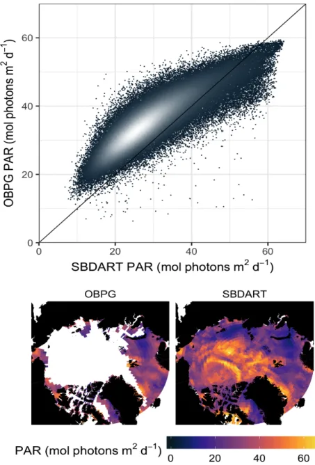
Archipelago and Baffin Bay (II), the Greenland and Norwegian Seas (III), the Barents and Kara Seas (IV), the Laptev and East Siberian Seas (V) and the Central Arctic Ocean (VI) are presented. Median sea ice concentration between May 21 and July 23 over 2000-2016 was added as a reference. ... 22 Figure 1.3 Comparison between two PAR products a) Scatterplot showing the comparison between SBDART and OBPG products over the Arctic open ocean for the 2000-2016 period, with the solid black line as the 1 to 1 correspondence. b) Example maps of both products for the 15 July 2010. ... 25 Figure 1.4 Ed(PAR) time series. The incident irradiance at the top of the atmosphere, and
under clear and observed skies for six Arctic regions over a 15-year period (2001 is removed because of a gap in the data) after a moving median with a window of seven days was applied to the time series. The black dots represent the day of annual maximum (DAM) for each time series of Ed(PAR, 0+). At the bottom, the boxplots
compile the distribution of the DAM, with the beginning and end of the grey boxes showing the interquartile range. The vertical dashed black line is the date of the summer solstice. ... 27 Figure 1.5 Median atmospheric transmittance. The atmospheric transmittance of PAR (Ta)
for 2000-2016 as a function of the day of the year for each of the six Arctic regions is shown in red. The green line at the top of the panels represents the atmospheric transmittance for the clear sky scenario (Ta clear sky), and the dark blue line
represents the atmospheric transmittance for the open water scenario (Ta open
ocean). The thinner cyan line represents the corresponding albedo. ... 29 Figure 1.6 Individual effects on atmospheric transmittance. The isolated effects of sea ice
(orange) and clouds (purple) on atmospheric transmittance are computed. The sum of these opposing effects is shown with the grey ribbon. ... 30 Figure 1.7 Trends in atmospheric transmittance. Trends are presented over 2000-2016 for
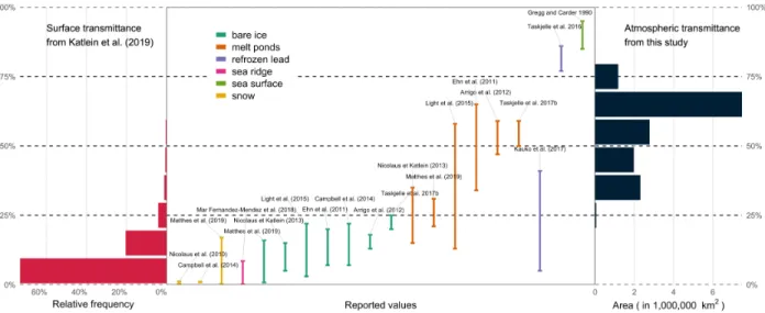
Spring: 6 June to 21 June, Early Summer: 22 June to 7 July, Summer: 8 July to 23 July), with a) all the annual median (25th and 75th percentile as error bars) and overlaid nonparametric regressions, and b) bar plots to quantitatively emphasize the slope sign and magnitude corresponding to the regressions in a), with a star to identify statistically significant slopes (p < 0.05). ... 31 Figure 1.8 Relative frequency distribution of surface PAR transmittance. Values are
computed from Katlein et al. (2019) (left), in the context of different PAR surface transmittances from previous studies (middle), along with the distribution of the Arctic PAR atmospheric transmittance per surface area (right). ... 34 Figure 2.1 MODIS spectral response. The three MODIS visible bands and their spectral
responses, shown with typical sea ice albedo values over the visible spectral range. ... 42 Figure 2.2 Green Edge study area. The 36 MODIS 500 m pixels are superimposed onto a
Landsat (30 m spatial resolution) true color image from USGS on 2015-07-14, and land relief from Natural Resources Canada (computed from a 5 m spatial resolution digital elevation model). The sea ice margin is around the second third of the image from the left. Inset shows the image location in the Arctic. ... 46 Figure 2.3 The MODIS surface reflectance quality control. The product L2G format
preserves all the observational data (up to 14 per day). The 36 pixels observations is the same as depicted in Figure 2.2, but stacked to represent all daily satellite passes. Each satellite pass contains 36 reflectances, quality indicators and associated sun-satellite geometry. Quality control, including the removal of cloudy scenes, highly reduces this number. ... 48 Figure 2.4 In situ ARF described in the in situ surface reflectance subsection. All sun
zenithal angles were close to 57°. The full angular resolution ARF from
measurements of three contrasted surface types and the three MODIS bands (01, 03, 04 at 613 - 682 nm, 538 - 569 nm and 451 - 481 nm, respectively) are shown.
Viewing azimuthal (0° to 360°) and zenithal (0° to 60°) angles are shown on a single plot, along with the black dots representing all MODIS Aqua and Terra viewing geometries at the Green Edge Site over the 2015 and 2016 studied period. The common color scale diverging palette allows seeing where the isotropic assumption underestimates (green) or overestimates (red) visible albedo. ... 50 Figure 2.5 Simulated ARF. The ARF polar plot from the simulated dataset are shown. One
simulation per category is presented, chosen to be the one with the middle of the three varying physical thicknesses with a sun at 55° and the zenithal viewing angle restricted to less than 60°. The main characteristic for the first row is the presence of a dry snow surface of 0.05 m snow that has a density of 320 kg m-3 and a snow grain
effective radius of 300 microns. For the second row, the melting snow had the same thickness but a density of 400 kg m-3 and a grain effective radius of 1000 microns. In
the third row, the bare ice case had 0.02 m of surface scattering layer (here
represented by old snow): 500 kg m-3 density, a grain effective radius of 1200 microns
on top of a layer of ice of 0.50 m of ice. The last row shows the melt ponds, with 0.10 m of water sitting on 0.50 m of ice with an important brine volume fraction of 15% (effective radius of 600 microns). ... 52 Figure 2.6 All albedo values used in this study. Dotted and solid lines representing in situ
derived (3) and simulated albedo spectra (36) that represent Arctic first-year sea ice. ... 53 Figure 2.7 Example of measured ARF values. a) Distribution of ARF values for in situ dry
snow case in the band 04 (538 - 569 nm) for the restricted zenithal range in white (all azimuthal angle, zenithal angle below 60°) and for the specific azimuthal viewing range of the two MODIS sensors typical of viewing direction encountered in the Arctic
(between 50° and 80° for Aqua and from 100° to 130° for Terra, with the zenithal angle below 60°). b) Display of these ARF values for the specific azimuthal range of Aqua viewing geometry, with the zenithal dependence. ... 55 Figure 2.8 Relationship of modeled and known albedo. The scatterplot shows the
comparison between the albedo predicted by our model and the known albedo from radiative in situ data (squares) transfer simulations (triangles), with the dashed line as the 1:1 ratio. The color code represents the different cases. ... 58 Figure 2.9 Albedo, its spatial heterogeneity and ancillary variables at the Green Edge Ice
Camp. In A and F, black dots are days with satellite-derived albedo data, derived from the multiple daily MODIS observations of surface reflectance. In B and G, dot size represents the number of valid satellite passes used in the computation of the visible albedo and the presented coefficient of variation. Other independently measured variables are: in situ albedo (empty squares - A and F), the near-surface air
temperature measured in situ (solid line in C and H), the melt pond coverage derived from photographs (black dots in D and I, with dashed lines representing the linear interpolation) and snow and rain events in E and J evaluated at the local airport. .... 60 Figure 3.1 A portrait of sea ice surface evolution on site for 2016, shown as the
near-surface air temperature in grey and daily binning in blue (top), and corresponding photos of the ice camp area used as an ancillary source to qualitatively describe the GES 2016 evolution (bottom), a) dry snow, 2016-05-27 at -1,9°C b) melting snow, 2016-06-11 at 1,7°C, c) first-year bare ice and light blue ponds, 2016-06-17 at 1,8°C, d) first-year bare ice and blue melt ponds 2016-06-30 at 3.9°C, e) first-year bare ice and dark blue melt ponds 2016-07-12 at 1,3°C and f) ice breakup 2016-07-21 at 14,2°C - Investigators: Haas C. (photos), Massé G. (air temperature). ... 73 Figure 3.2 Satellite passes used a) in the model in 2016 b) comparison of modeled and
measured PAR values with the dashed lines representing a 20% difference and the color of the dots is the coefficient of variation of PAR during the recorded sequence. ... 76 Figure 3.3 Estimated PAR at the different levels of the atmosphere-ocean system for the
years 2015 and 2016. Potential PAR is colored according to different percentages of loss due to absorption. ... 77 Figure 3.4 Potential PAR with overlaid measured depth-integrated chl-a from the sea ice
and water column. ... 79 Figure 3.5 Total PAR budget in a single layer of ice, with the reflected, transmitted and
loss due to absorption calculated every time the ice thickness was increased by 0.01 m. The horizontal black line indicates the depth at which the part that is reflected stops changing. ... 82 Figure 3.6 Potential PAR with overlaid measurements of PAR (0-). ... 84
Figure 4.1 Sea ice brightness temperature and corresponding visible albedo for the years 2013 to 2016 in the Arctic. ... 89 Figure 4.2 Image of the Green Edge site captured from the Sentinel-2 MSI sensor at 10m
spatial resolution. The Green Edge site is identified with the grey circle. Surrounding the site are brown rocky landscapes. The sky is clear over the site of interest. However, clouds are visible on the Western side of the image, potentially impacting the light availability on the Green Edge site. ... 91 Figure 4.3 Modeled evolution of the cryosphere at the Green Edge Site. Four stages are
identified: premelt, melt, ponding and open waters. In this model, the sea ice
transmittance excludes sympagic algae. The cartoon was based on the work of Julie Sansoulet. ... 93 Figure 4.4 Comparison of the area-averaged transmittances and the transmittance from
Figure 4.5 Typical transmittances of the premelt (5 May), melt (13 June), ponding stages (25 June). Histograms have bin width of 0.5 %. ... 98
Liste des tableaux
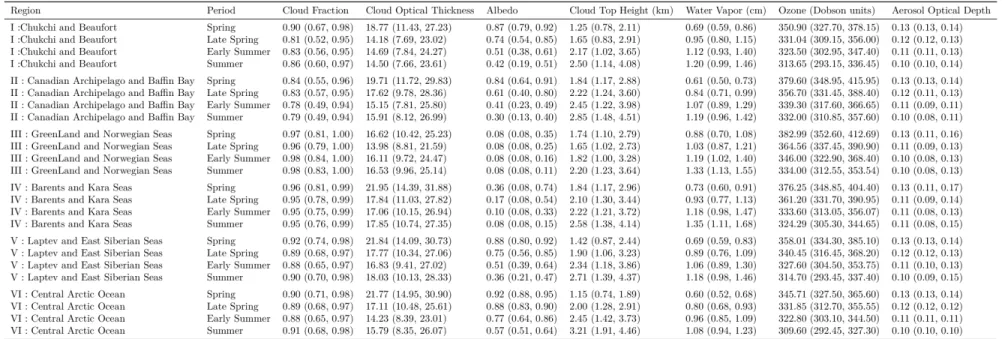
Table 1.1 Products used to derive Ed(PAR, 0+). Products, associated references, spatial/temporal resolutions, time span and website of the satellite-derived inputs used to compute the above surface downward irradiance are presented. ... 20 Table 1.2. Values used as input for the simulations. The median values (interquartile
range) are derived from satellite and are used in the SBDART simulations over 2000-2016. ... 24 Table 2.1 Statistics for the different ARF origins, cases and type. The standard deviation
result from ARF values when all hemispheric values are included (model only), when values are restricted to viewing zenithal angle below 60° and also when only MODIS-specific azimuthal range is included. ... 56 Table 3.1 Monthly average of cloud index, albedo, minimum and maximum PAR derived
from the model ... 78 Table 4.1 Layer components per stage ... 94
Liste des abréviations et symboles
Abréviation Nom complet
chl-a Chlorophyll-a
PAR Photosynthetically available radiation
Ed(TOA, PAR) Top of the atmosphere downwelling planar
irradiance of PAR
Ed(0+, PAR) Above surface downwelling planar irradiance
of PAR
Ed(0-, PAR) Below surface downwelling planar irradiance
of PAR
NASA National Aeronautics and Space
Administration
ESA European Space Agency
JAXA Japan Aerospace Exploration Agency
Avant-propos
Cette thèse comporte cinq sections : une introduction générale, trois chapitres de résultats scientifiques sous la forme d’articles, et une conclusion générale. Les trois chapitres de résultats scientifiques sont rédigés pour être publiés dans des revues à comité de lecture. Deux des trois chapitres ont récemment été soumis dans une même revue. Le troisième n’est pas encore soumis. Mon rôle dans la préparation de ces articles consistait à conceptualiser les études, faire les analyses associées, positionner la recherche par rapport aux recherches précédentes, présenter les résultats, discuter de ces résultats et réfléchir aux efforts futurs.
Laliberté, J., Bélanger, S. et Babin, M. (2020), The transmittance of the atmosphere for the photosynthetically available radiation over the Arctic Ocean, Elementa: Science of the Anthropocene, Article soumis le 06/30/2020, (ID: b9666d043e63988d)
Laliberté, J., Rehm, E., Hamre, B., Goyens, C. et Babin, M. (2020), A simple method to derive a satellite visible sea ice albedo time series over the Arctic Ocean, Elementa: Science of the Anthropocene, Article soumis le 06/29/2020, (ID: 5636f89c5c87452c)
Laliberté, J. et Babin, M. (2020), Satellite-derived potential PAR availability for marine primary producers at the ice-covered Green Edge Site, Article en préparation.
Introduction
While some researchers scan the outer space for a life form, others are still trying to figure out the mysteries of indigenous life. Life on our planet is ubiquitous. A tremendous breakthrough has been achieved by launching Earth observing satellites, and, ever since, monitoring the patterns of nature through time and space has become much easier. Yet, there is still much work to do to understand it, and on a personal note, I think that is a wonderful way to spend time.
Phytoplankton
Phytoplankton, microscopic drifting organisms in the World Ocean, can be observed from space. Their presence spans all ocean and lake surfaces, that is, 71% of Earth's surface. They can be found in very low concentration (0.01 mg m-3 of chlorophyll-a, a common
biomass index for microalgae in seawater) in desertic oceans, or in very high concentration (>10 mg m-3) in nutrient rich areas. Phytoplankton harvest sunlight using their photosynthetic
apparatus. This complex process releases oxygen allowing other organisms (e.g., us) to breathe. They fix inorganic carbon which is incorporated in hydrocarbons, lipids, proteins and nucleic acids. Field et al. (1998) estimated that inorganic carbon was roughly incorporated in equal parts in land and ocean plant biomass. When phytoplankton end their life, they are either recycled in the enlighten, topmost part of the ocean, or they go down into the deep sea below (e.g., export production shown in Table 5 of Laws et al. 2000). When primary producers are ingested by grazers, this carbon is passed along and allows other organisms to grow and reproduce. This is the start of the long and complex marine food web. When this submarine plant material sinks, before or after its ingestion (fecal matter), microorganisms in the deep-sea break it into inorganic compounds. Ultimately, ~0.1% of the total carbon fixed at the ocean surface is buried in the sea floor, and over Earth’s second half of its 4.6-billion-year history, this process shaped today’s environment chemical composition (Falkowski, 2012).
Coal from land vegetation along with fossil phytoplankton is what we’ve been using as our primary energy source for the last centuries to sustain our rapidly growing population. Consequently, in the very recent geological times, humans also played a major role by transferring a lot of these prehistoric organisms into the atmosphere in the form of greenhouse gas (transmits the radiated energy from the Sun, absorbs the irradiated energy from the Earth), inducing global warming. Interestingly, global warming also influences
natural fluxes of carbon. For example, it may have started to slow the pulling of carbon into the deep ocean on a planetary scale (Le Quéré et al. 2010).
It was shown that during the last decades, the upper layer of the temperate latitudes oceans is warming. This implies a reduction of mixing with the cold waters of the depths. This strengthened stratification is limiting the vertical exchange of nutrients. Consequently, phytoplankton are less present and most of the Global Ocean absorbs less inorganic carbon (Behrenfeld et al. 2006). Most, but not all, as intake fluxes from polar regions could potentially benefit from this warming. For instance, the increasing duration of the ice-free season from year to year could make the Arctic more productive (e.g., Arrigo and Van Dijken, 2015).
Changes in the Arctic
This rapid warming and its close linkage to the rise of anthropogenic atmospheric carbon are worrisome. In particular, the Arctic Ocean is changing rapidly in comparison with the rest of the planet (Serreze and Barry, 2011). Because the Arctic atmosphere and surface respond in complex and entangled ways, it is hard to understand and forecast the fate of the future Arctic Ocean. Without going into details, we can easily understand why by listing some of the mechanisms at work.
The amount of energy from the Sun that reaches the Arctic Ocean interior increases with the melting of the sea ice, which in turn heats seawater and causes the ice to shrink and thin out. Less and less ice survives the summer because of the warmed air and water surrounding it. Lower sea ice areal coverage and thinner ice means more energy from the Sun is absorbed into the ocean (Kashiwase et al., 2017). This delays the fall freeze up, the seasonal ice does not grow as thick during the winter and so forth (Stroeve et al., 2011). But then, with more of the ocean exposed to the Sun's radiation, the evaporation of water is increased, moisture promotes cloud formation, and the incoming energy from the Sun is more readily reflected (He et al., 2019). Yet, clouds trap Earth’s radiative emissions (longwaves) which contribute to more sea ice melt (Perovich, 2018). With these processes to model (and many more), the error budget can become quite large, and the fate of the future Arctic remains uncertain.
Studying observations is easier than making projections about the future. This is what I focus on in this thesis. Of major interest are satellite observations. A massive amount of satellite
imagery captured snapshots of the environment over the years. This really helped to reveal the extent of recent changes in the Arctic Ocean. For instance, for over 40 years, the surface brightness temperature of the Earth has been monitored, and this information can be converted into sea ice concentration (SIC) and sea ice age (SIA) (a good indicator of sea ice thickness). Let me illustrate through an example how these observations can provide undeniable evidence of climate change. I was born in 1987. I started my thesis in 2016. The difference in SIC and SIA over this period is striking (Figure 0.1).
Figure 0.1 Mean sea ice concentration for the years a) 1987 and b) 2016, as well as the mean sea ice age for the years c) 1987 and d) 2016. Both products were obtained from the NSIDC (product code nsidc-0051 from Cavalieri et al. (1996), product code nsidc-0611 from Tschudi et al. (2016)). There is a hole at the pole due to the limits of the coverage for the satellite sensors (SMMR, SSMI, and SSMIS). In the sea ice concentration product, I set the hole to a 100% ice cover, whereas the NSIDC had already filled the sea ice age gap with an interpolation guided with ancillary data (buoys and other satellite sensors). The land topography was obtained from the polar geospatial center (Porter et al. 2018).
Looking at these images, it also seems very likely that Arctic primary production was altered over recent times. Less sea ice can influence nutrients and light available in the marine environment (Tremblay et al. 2015). As of today, appraising the consequences of these environmental changes on Arctic primary production, and all the ecosystems that depend
on it, remains a challenge (McGuire et al. 2009, Popova et al. 2012, Manizza et al. 2013, Vancoppenolle et al. 2013).
Arctic marine primary production
In the Arctic, the long-lasting winter hampers primary production and allows nutrient replenishment through mixing. Typically, nutrients are recycled at depth, and in the winter, when the ice forms, the dense, cold and salty water (salt rejection from ice formation) sinks down, and this convection transports the nutrients back to the surface. The water column is then filled with nutrients such as nitrates that support and control primary production (Tremblay et al. 2011, Mills et al. 2018). The mixing is reduced in the spring. On the one hand, solar radiation directly heats up the ocean in open areas like leads and in the marginal ice zone to create a temperature gradient. On the other hand, this warmer water causes lateral and bottom melting of the ice, resulting in an important salinity gradient. Spring solar heat input directly into the ice also allows stratification through melt water release, stabilizing even more the water column. In that way, the return of the sun allows drifting photosynthetic organisms to grow without being pulled towards great depths where not enough sunlight is present.
Given these nutrients are available and that the water is stratified enough, phytoplankton will photosynthesize when the light returns. In fact, every spring when the Sun comes back from a long absence, populations of phytoplankton erupt in massive growth. This sudden and transient abundance is called a spring bloom and is terminated by nutrient depletion and/or grazing being stronger than growth. It is by far the greatest primary production event of the year and it massively fuels the ecosystem with energy (Perrette et al. 2011). In particular, the timing of the bloom is really important for all life that depends on it (including migratory species). Can we monitor this phenomenon? In short, in open waters, the bloom can be observed by satellites. In ice-covered waters, it has to be inferred.
Ocean color remote sensing
Sampling the Arctic Ocean by hand is not easy. It is expensive, remote, vast and dangerous. Opportunities are rare and irregular. Here and there, when cruise ships go north, observers can provide some information on the state of the primary production. For instance, incubation on-board cruise ships can be used to assess the rate of carbon uptake by marine primary producers. This surely helps understand how Arctic primary production works but
lacks the temporal and spatial coverage needed to assess how much ‘food’ there is in the Arctic Ocean over time.
Arctic-scale assessment of open water primary production is possible from satellite remote sensing. The ocean color remote sensing approach to estimate primary production is based on the retrieval of chlorophyll-a concentration, an indicator specific to the presence of phytoplankton. Estimates of chlorophyll-a are well correlated with phytoplankton biomass and are the primary input in primary production models. As listed in the IOCCG report 16 (2015), ocean color remote sensing can be challenging in the Arctic because of the persistent cloud cover (Perrette et al., 2011), the prevalent low solar angle and the contamination of the satellite-measured signal by the highly reflecting sea ice (Bélanger et al., 2007). Additionally, the Arctic Ocean has extended continental shelves harboring optically complex waters (Bélanger et al., 2008), for which the vertical distribution of the chlorophyll is different from what is found in the Global Ocean (Ardyna et al., 2013). Also, in the primary production models, phytoplankton must be represented by photosynthetic parameters that are specific to this unique environment (Bélanger et al. 2013). In fact, Lee et al. (2015) evaluated 32 ocean color models in the Arctic Ocean with in situ daily production and found that the root mean square difference ranged between 0.6 and 0.8 mg C m−2 d-1,
which is much greater than the 0.1 to 0.5 mg C m−2 d-1 range obtained in their previous model
intercomparison efforts for temperate latitudes. On the bright side, sunglint is not a problem for satellites scanning the Arctic, and satellite overpasses are frequent.
For 21 June 2015, a day of expected minimum low solar angle problem, I downloaded all the data collected over the Arctic by the MODIS sensor (on-board the Aqua satellite, completing approximately 14.5 orbits per day, data available from the Ocean Biology Processing Group website: https://oceancolor.gsfc.nasa.gov/). The ancillary data from microwave satellites (included in the standard processing of the chlorophyll retrieval) indicated that 70% of the Arctic pixels had an ice concentration greater than 10% (yielding no valid chlorophyll retrieval over that area). Even with so many swaths to increase the chances of viewing the water surface, 90% of all the Arctic Ocean was covered by sea ice and clouds. In fact, for these images on average, 99 % of the Arctic Ocean yielded no
chlorophyll values. This makes studies on biological cycles (also named phenological studies) very difficult to carry.
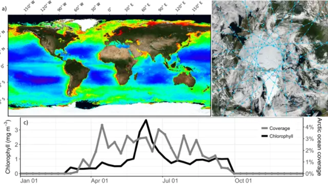
Figure 0.2a presents the global chlorophyll concentration binned over a whole year, illustrating the full potential of ocean color over the open ocean. Figure 0.2b shows the remarkably large potential of coverage available from the Aqua orbital track over the Arctic Ocean (Aqua completes an orbit in about 99 minutes). In spite of this, Figure 0.2c shows that even when weekly binned images are used, the surface coverage is rarely above 3% (this includes sea ice). That shows why, in general, ocean color data obtained from satellites fails to provide the necessary information to build a representative picture of what is going on in terms primary production in the Arctic Ocean.
Figure 0.2 Potential of ocean color satellite data in the Arctic. a) Chlorophyll concentration yearly composite for the year 2015, b) Satellite passes for MODIS-Aqua on 21 June 2015, c) Availability of ocean color sensor coverage from 2015 weekly composites and associated mean chlorophyll concentration.
Nonetheless, this is the most powerful tool to monitor phytoplankton primary production response to environmental changes. Using ocean color remote sensing, Arrigo and Van Dijken (2015) estimated that in open waters, productivity of the Arctic Ocean has increased by ~2% per year over 1998-2012. Bélanger et al. (2013) estimated an increase of ~1.4% per year over 1998-2010. This is a strong and rapid change. But what is most important is that the timing of the production is shifting in time and magnitude (Renaut et al. 2018), and
this can really perturb the transfer of energy in the marine food web (Leu et al. 2011, Platt et al., 2003).
In summary, to this day remote sensing greatly helped improve our understanding of the dynamics of phytoplankton in open water Arctic environments, but evaluating the immediate response in primary production over high latitudes to the contemporary changes in climate remains a challenge and will require tremendous endeavor and innovative techniques to reveal its patterns and underlying mechanisms (Leu et al. 2015, Behrenfeld et al. 2017). A lot is going in open waters, but many researchers are also convinced a lot is going on where the satellites cannot probe (e.g., Zhang et al. 2010).
Ice-covered waters
Key variables traditionally derived from passive satellite imagery to derive pelagic primary production are impossible to capture under sea ice because the frozen surface layer acts as a highly diffusing barrier that blurs and reduces the light transfer between the atmosphere and the ocean beneath. But phytoplankton can bloom under the ice. Under-ice productivity has even been documented for quite some time (Legendre et al. 1981, Gradinger 1996, Strass and Nöthig, 1996, Yager et al. 2001, Fortier et al. 2002). In most cases the level of productivity was judged moderate and it was not recognized as an important phenological feature. Also, perhaps it was difficult to ascertain that the measured chlorophyll really had grown in the water under the ice. However, in 2011, the ICESCAPE (Impacts of Climate on EcoSystems and Chemistry of the Arctic Pacific Environment) cruise captured an event of unexpected breadth in the Chukchi Sea (Arrigo et al. 2012). Below a one-meter-thick ice cover was hiding a 30 m thick layer of thriving, highly concentrated phytoplankton (up to 30 mg chlorophyll-a m-3), a concentration much higher than the global average (0.19 mg m-3)1.
The scientific crew aboard the icebreaker had to make sure the biomass had not been released from the ice above, or advected from the ice-free ocean some distance away. The pattern of chlorophyll-a in relation to the direction of sea ice retreat as well as the species composition and the depth of nutrient depletion suggested that the massive chlorophyll-a concentration found there had not been released from the ice matrix. It simply grew under the consolidated ice cover. Their analysis led to believe that the phenomenon had started
1 This is the median value I computed from the entire MODIS-Aqua mission composite,
because of sustained light availability, as ponded sea ice transmits a higher amount of visible light than thick ice (Palmer et al. 2014).
We do not know if under-ice blooms are widespread (Figure 0.1). No straightforward solution to identify these blooms is practicable except to go out in these remote areas and measure primary production. To identify under-ice bloom on a rather local scale, ice camps (Oziel et al. 2019, Mundy et al. 2014), oceanographic cruises (Randelhoff et al. 2019, Arrigo et al. 2014), ice-tethered buoys (Hill et al. 2018, Laney et al. 2014), bio-Argo floats (Mayot et al. 2018) and even sediment traps (Fortier et al. 2002) can be used. In addition, in the near future, acoustic positioning should help decrease the risk associated with sea glider deployments in ice-covered waters (Eric Rhem, personal communication, May 2020). When considering the problem at pan-Arctic scale, however, the observation network built from all these cumbersome, expansive direct observation techniques would greatly benefit a more comprehensive view of the matter. Primary production in ice-covered waters must be studied from indirect observations.
Arctic light
The populations of Arctic microalgae may be damaged by the ultraviolet sunlight (Cullen and Lesser 1991, Perovich, 2006) or indirectly profit from the thermal radiation that increase sea ice melt or water temperature (Cherkasheva et al. 2014). Yet, of all solar radiation, the main spectral range impacting the microalgae is the visible portion of the electromagnetic spectrum, named PAR (photosynthetically available radiation). The amount of PAR reaching the top-of-the-atmosphere can be computed precisely and considered exempt of error. The environmental factors further reducing Arctic PAR can be divided into two layers, the atmosphere and the surface, such that the PAR at the top of the water column is the top-of-the-atmosphere PAR multiplied by the transmittance of the atmosphere and that of the surface. These layers are subject to strong spatiotemporal variations and studying their radiative effect is important to understand the annual cycle of light available at the top of the water column. The atmosphere is composed of gases, aerosols and clouds. The surface is made either of the air-ocean interface, or of sea ice (mainly snow-covered ice, bare ice or pond covered ice). The effect on light propagation of these environmental features can be deduced from satellites and radiative transfer models.
It is in the leads or in the marginal ice zone that marine daily PAR reaches the highest values encountered anywhere in the Global Ocean. This can be shown by using an atmospheric
radiative transfer model. For a polar latitude of 74° on 1 June (e.g., middle of Baffin Bay when the ice retreats) under a clear sky and typical Arctic atmospheric conditions, the computed above surface incident PAR is 63 mol photons m-2 d-1 in open waters. For the
same atmospheric conditions and a linear mixture of snow-covered sea ice (90% areal fraction) and open water albedo (10% areal fraction), it reaches 69 mol photons m-2 d-1. Long
enlighten days combined with multiple surface-atmosphere reflections is generating extreme daily PAR values. Under the right cloud configuration, this can even be boosted (Rabette and Pilewskie 2002). To put these numbers in perspective, for the same date of this year (2020), the mean value between the tropic of Capricorn and the tropic of Cancer was 43.2 mol photons m-2 d-1 and the clear skies’ value reached a maximum of 63.4 mol photons m-2
d-1.2
For phytoplankton drifting under an ice field interspersed with leads, the contrasted light conditions are astonishing. Taking the PAR values from the above paragraph (69 mol photons m-2 d-1), it is plausible that snow atop sea ice reduces surface transmittance down
to less than one percent, while open water (leads) transmit more than 90% of the incident light. Over a few horizontal meters, marine light can change from ~0.6 mol photons m-2 d-1
to ~60 mol photons m-2 d-1. The same is true with melt ponds and bare ice, although less
extreme because the two surface types have less contrasted transmittance (typically 15% and 55%, respectively, e.g., Arrigo et al. 2012). Primary producers have adapted to this peculiar light regime profoundly altered by the changing atmosphere and surface, ranging from total polar night to never-ending summer solstice light exposure, undergoing shallow to very deep mixing. At low light levels encountered under a consolidated ice cover right after the polar night, the shade-adapted phytoplankton can photosynthesize (Kvernvik et al. 2018, Morin et al. 2019). Surprisingly, at high light levels, they may also photosynthesize (Lacour et al. 2018, Assmy et al. 2017). In fact, phytoplankton was observed to have acclimated to very different light levels even over small spatial and temporal scales (Palmer et al. 2013, Kauko et al. 2019). This photoacclimation is also adaptative over the seasonal cycle of light, with the phytoplankton population being more efficient at using light during the spring (nutrient-rich waters) than their counterparts encountered after the bloom period (nutrient-limited waters) (Lewis et al. 2019).
2 I computed these statistics from the MODIS-Aqua daily PAR product,
Modeling Arctic light
Information on the shortwave radiation partition for the atmosphere (Curry et al. 1996, Barrientos Velasco et al. 2020) and the surface (Ebert et al. 1995, Lu et al. 2018) has been modeled for a long time but is it still an active field of research. It is generally used to reveal the energy balance in the Arctic. However, the partitioning specific to the PAR spectral range is much less studied.
Coupled physical–biological sea ice/ocean models may be used to inquire on under-ice primary production in polar regions and have provided great insights about primary production in the Arctic Ocean (Lavoie et al. 2009, Jin et al. 2012, Ji et al. 2013). For instance, Popova et al. (2010) and Clement Kinnery et al. (2020) suggest the under ice production could account for 35 to 45% of the total Arctic production. Yet these models also have several limitations (Babin et al. 2015). For example, models often have to use proxies to represent certain unavailable variables, resulting in a poor representation of light availability in primary production assessment (e.g., Dupont (2012), like many others, used a broadband shortwave irradiance product converted to visible wavelengths using a fixed value of 0.43, notwithstanding sky conditions). Also noteworthy is the use of coarse grid cells with an absence of sub-grid variability that can become a severe hindrance when computing the non-linear vertical light attenuation. This may lead to large uncertainties when fed to the model. Moreover, the attenuation in sea ice is often parametrized crudely (Briegled and Light, 2007).
In a modeling study, Horvat et al. (2017) investigated the distribution of potential light-limited bloom events. In their model interpolated at 0.5° x 0.5°, the light available at depth z in the water, I(z), is obtained from
!(#) = !! (1 − )) *"#!$ *"#"%
Equation 0.1
with !! as the incident light, ) as the albedo of the surface (ratio of reflected to incident light),
h and z as the sea ice and water thicknesses, and +& and +' as the sea ice and water
extinction coefficients, respectively. To express light availability under sea ice (!(#)) they used constant albedo values for snow (0.98), bare ice (0.76) and ponds (0.2). They also used constant extinction coefficients of 1.6 m-1 for sea ice and of 0.12 m-1 for water. They
conversion from shortwaves to PAR was not discussed. The ice thickness and melt pond fraction were derived from the Los Alamos Sea Ice Model (CICE). They compared ice thickness and melt pond fraction and concluded that, of the two, ice thickness was more important for sub-ice blooms. This, of course, depends on how the sea ice transmittance is modeled. So, models are useful, but more constraints from satellite-derived information (e.g., incident PAR, PAR albedo) could surely improve this static and oversimplified view of nature.
Lange et al. (2017) used a similar approach to map suitable habitats for ice algae at a pan-Arctic scale. Their approach was somewhat more satellite oriented. It was based on a 25 km x 25 km monthly ice thickness product, derived from the synthetic aperture radar altimeter with snow depth from a climatology. No incident energy was used. They simply focused on sea ice transmittance. One extinction coefficient for snow and one for ice were assumed. They used constant albedo values for snow (0.81) and bare ice (0.70). Again, this underlines how researchers are limited by not having a way of retrieving the seasonal evolution of PAR albedo and incident PAR at scales that allow to sufficiently resolve under-ice light-limited primary production activities.
Assmy et al. (2017) carefully studied the environmental conditions and associated phytoplankton biomass on a drifting ice-floe between the Fram Strait and Nansen Basin. They documented an important under-ice bloom. The nutrient depletion at depths down to 50m indicated drawdown from phytoplankton and not by ice algae. Their analysis of in-ice and in-water communities suggested the same conclusion. Finally, their observations and models of water currents do not show evidence of advection from the ice edge. They monitored the surrounding lead fraction using a supervised classification of Synthetic Aperture Radar images. The light at depth z in the water was calculated using the same approach as presented above, that is the albedo and extinction coefficient are used to reduce the incident light (see their supplementary information). The incident PAR was measured, and three different surface types had an albedo and an extinction coefficient assigned: open water, thin ice with thin snow cover and thicker ice with thicker snow cover. For each surface type, constant extinction coefficients were used (one for snow, one for ice). These coefficients were obtained from their transmittance measurements. At last, the extinction coefficient used to propagate light in the water was parameterized as an empirical function of the measured chlorophyll-a. Unfortunately, the PAR albedo values they used are not presented. They concluded that the light level necessary for spring blooms comes from
leads, at least in the Fram Strait and the Barents Sea for the present-day Arctic, and that leads may initiate spring blooms in the whole Arctic in the future.
From this review (Arrigo et al. 2012, Lange et al. 2017, Horvat et al. 2017, Assmy et al. 2017), what do we gather? First, all the papers presented above agree that under-ice primary production is light-limited, and all focus on the change in sea ice transmittance. None specifically addressed the role of light transmission by the atmosphere. Second, the light transmittance modeled as a function of albedo, sea ice thickness and extinction coefficient (Equation 0.1) is well-established in the literature. Most of the time, it would benefit from an albedo value resolved in time and space, either locally or across the Arctic. Finally, if we want to understand under-ice spring bloom dynamics, incident irradiance values appropriately computed for the PAR range must be calculated at a spatiotemporal scale meaningful for phytoplankton.
Research objectives
We now know that the ice-covered Arctic can support blooms of impressive magnitude. Could we use the information regarding the light availability to infer their presence? The thesis general objective is to better constrain the under-ice light regime and its dynamics. This thesis is based on the premise that, regardless of nutrients, studying potential under-ice irradiance at a pan-Arctic level could provide means to know more on the under-under-ice phytoplankton bloom dynamics.
In the first chapter, we examine the transmittance of the atmosphere layer over the Arctic. For simplicity, the Earth system is often modeled as two vertically stratified slabs of infinite extent, the atmosphere and the ocean. In recent Arctic under-ice bloom studies, the focus was generally on the ice-covered ocean and changes in response to the recent warming, while the atmosphere received little attention. We know that the visible sunlight is more readily transmitted through the surface of the Arctic Ocean than before. We want to know if this is also the case for the atmosphere.
In the second chapter, we develop a model that could be used to obtain the visible albedo of sea ice from satellites. Methods to process this variable over the spectral range of interest are lacking, so we conceptualized and implemented a simple way to derive how much PAR is neither transmitted nor absorbed within sea ice using satellite remote sensing. The method provides an albedo estimate at spatial and temporal resolutions desirable to inquire on primary production.
In the third chapter, we develop a method to estimate how much PAR reach the surface. Combining this method with what was developed in the second chapter, we can constrain the potential PAR available for phytoplankton in the Arctic Ocean. The method is designed to be implemented over the entire Arctic.
1 The transmittance of the atmosphere for the
photosynthetically available radiation over the
Arctic Ocean
J. Laliberté, S. Bélanger, and M. Babin
1.1 Résumé
La plupart des études sur la phénologie du phytoplancton sous la glace ne reconnaissent pas les variations de l’atmosphère terrestre en tant qu’acteur dans le cycle annuel de la lumière sous-marine. La littérature scientifique décrit généralement les variations de régime lumineux sous-marin avec une emphase sur la neige, la glace, les chenaux et les mares de fonte, qui, à un endroit ou à un autre, rétrécissent, se fragilisent ou deviennent plus transparents, mais sans mentionner l’effet potentiel des nuages ou du brouillard. Pourtant, nous savons que ces derniers augmentent avec le retrait de la couverture de glace au printemps et à l’été, lorsque le soleil atteint sa force maximale. Quelle est l’importance de l’atmosphère pour la lumière sous-marine? À l'aide d'observations par satellite, d'observations sur le terrain et de modèles, nous avons évalué l'importance des variations de l’atmosphère dans le contexte des variations de la glace de mer qu’on retrouve à la surface de l’Océan. Notre travail révèle que l'atmosphère arctique change et devient moins transparente à raison de 2 % par décennie, à cause de l'augmentation de la nébulosité et de la diminution de l'interaction radiative entre l'atmosphère et la surface. Une étude plus approfondie sera nécessaire pour savoir à quel point cette tendance compense pour la glace de mer qui devient plus transparente avec les années.
1.2 Abstract
The Arctic atmosphere-surface system transmits visible light from the Sun to the ocean, determining the annual cycle of marine light available to micro-algae. A known consequence of Arctic warming is the increase in the Arctic surface transmittance, but much less is known about the Arctic atmosphere transmittance. Because Arctic primary production is often driven by visible light availability, we investigated the variations of the atmospheric transmittance at a pan-Arctic scale between 2000 and 2016. We combined a large dataset of atmospheric and surface Arctic conditions into a radiative transfer model and found that typical atmospheric transmittance ranged between 60% and 70%, being much larger than the typical sea ice transmittance. We also found that Arctic atmospheric transmittance decreased at a rate of 2.3%/decade over the studied period, in part due to the increase in
cloudiness, in part due to the weaker radiative interaction between the atmosphere and the surface. Further investigation is required to know if this negative trend compensated for the positive trend in sea ice transmittance.
1.3 Introduction
In the Arctic marine ecosystems, light limits primary productivity during several months of the year, especially during the polar night. During other times of the year, sea ice (including overlying snow) is what constrains most the amount of photosynthetically available radiation (PAR) in the water column. The impacts of ongoing climate-related changes on sea ice transparency to PAR have been emphasized in several recent studies (e.g., Horvat et al., 2017, Assmy et al., 2017, Arrigo et al., 2012). Significant reduction in the atmospheric transparency to PAR has also been observed at the pan-Arctic scale, impacting the marine primary production (Bélanger et al. 2013). Bélanger et al. (2013) PAR estimations at the sea surface, however, ignored the radiative interaction (i.e., multiple back and forth diffuse reflections) between the atmosphere and the highly reflective surface in the presence of sea ice. Laliberté et al. (2016) included this interaction in their PAR model and based on in situ observations, showed its significance. Here we further examined the variations in atmospheric transparency over the Arctic Ocean while taking into account the interactions between the atmosphere and surface. We focus on the spring-to-summer transition when both the ocean surface and the atmosphere change rapidly due to rising air temperature and melting snow and sea ice.
In this study, the surface is either defined as the air-ocean interface or includes sea ice, when present. We define the surface transmittance for PAR (Ts, %) as the ratio of downward irradiance integrated over the PAR spectral range (400 to 700 nm) in the water just below the sea or ice surface [Ed(PAR, 0-), mol photons m-2 d-1], and downward irradiance in the air just above the sea or sea ice surface [Ed(PAR, 0+), mol photons m-2 d-1]:
,
( =
-)(./0, 0")
-)(./0, 0*)∗ 100
Equation 1.1
Accordingly, the atmosphere transmittance (Ta, %) is defined as the ratio between Ed(PAR, 0+) and downward irradiance at the top of the atmosphere [E
d(PAR, TOA), mol photons m-2 d-1]:
,+ = -)(./0, 0*)
-)(./0, ,4/)∗ 100
Equation 1.2
Ts variations in the Arctic Ocean are mostly driven by changes in sea ice concentration and physical properties, including thickness, brine and air content, presence of melt water and the state of the snow cover (Arndt & Nicolaus, 2014, Perovich 2005). The most critical factors controlling variations in Ta are cloudiness (Rabbette & Pilewskie, 2002, Bélanger et al., 2013), and surface albedo (Grenfell & Perovich, 2004).
Sea ice cover and thickness are decreasing (Stroeve et al., 2011), while leads and melt ponds coverage are increasing (Flocco et al. 2012, Wang et al. 2016), resulting in an increase of Ts. In parallel, a general increase in cloudiness (Eastman & Warren, 2010) is especially noticeable in in the spring and summer (Wang & Key, 2003), resulting in a decrease in Ta. In this context, Ed(PAR, 0-) available to Arctic marine primary producers results from the balance between reduction of Ts and augmentation of Ta (Bélanger et al., 2013).
This work focuses on evaluating Ta over the Arctic Ocean. We decomposed the Arctic Ocean into six regions and the marine productive season into four periods of the year relevant to primary production and centred on the summer solstice. Using satellite remote sensing data from multiple sources combined into a radiative transfer model, we computed Ta over 17 years for each region and period of the year. Interannual and seasonal (phenology) trends were calculated and interpreted. Finally, we discussed the atmospheric transparency in the context of known variations in Ts.
1.4 Materials and Methods
1.4.1 Model
Ed(PAR, 0+) and Ed(PAR, TOA) were computed every day between 21 May and 23 July for every 1x1-degree pixel above the Arctic circle (66°N) for non-land areas between 2000 and 2016, resulting in 8640 pixels x 64 days x 2 estimates per year.
To compute Ta, we used SBDART (Santa Barbara Discrete ordinate Atmospheric Radiative Transfer, Richiazzi et al. 1998), a 1-dimension atmospheric radiative transfer model. The input variables were cloud fraction, cloud optical thickness, cloud top height, water vapour amount, total ozone amount, aerosol optical depth, and the surface albedo (see below). SBDART has been extensively used to propagate irradiance through the atmosphere (e.g.
Grenfell & Perovich, 2008, Su et al., 2007, Shupe & Intrieri, 2003, Painter et al. 2012). For each pixel, two SBDART runs were made every day, one for the clear part of the sky, the other for the cloudy part. They were then conservatively blended according to the cloud fraction. Each run yielded spectrally-resolved downward irradiance at a 3 nm spectral resolution and expressed in W m-2 μm-1. The instantaneous irradiance was then converted
to Ed(PAR, 0+) (mol photons m-2 d-1), assuming constant atmospheric and surface conditions throughout the day for the temporal integration (Frouin et al. 2003).
1.4.2 Inputs
All inputs from satellite data discussed in this section are summarized in Table 1. An atmospheric dataset was built from the MODIS Level 3 Atmosphere Gridded Product (MOD08 and MYD08, Platnick et al. 2017), which contains the diurnal (daytime) cloud fraction, cloud optical thickness, cloud top height, water vapour and ozone content, and aerosol optical depth (AOD) (https://modis-atmosphere.gsfc.nasa.gov/). These atmospheric properties were retrieved from multiple observations collected during different times of the day and averaged on an equal-angle global grid (Hubanks et al. 2019). We downloaded data from both Terra and Aqua platforms and averaged them to obtain daily fields on a pixel basis.
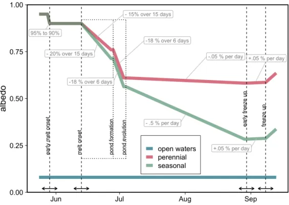
We generated a surface albedo dataset following a large-scale generic model of the seasonal evolution of albedo for the visible spectral range, modified from Perovich and Polashenski (2012) (see also Perovich et al. 2002, 2007, 2011; Light et al. 2014). This empirical model distinguishes six transitions in the state of sea ice during a year (Figure 1.1). It takes into account the sea ice age, sea ice concentration, and a number of melting or freezing phases that are detected from space using passive microwaves. The phases were determined from the dates corresponding to early melt onset, melt onset, early freeze onset and freeze onset (Markus et al., 2009). These onsets are based on surface wetness, monitored using the microwave signature of the surface. After winter, the early melt onset is the date when the sea ice surface layer wetness first increases. The surface layer then undergoes melt-freeze cycles for some time, but eventually reaches the melt onset, a state when sea ice persistently contains liquid water. The two other markers are the opposite, with the first occurrence of freezing conditions and the steady ones. The surface albedo was determined assuming specific sea ice albedo for each phase. When a pixel is ice-covered, its albedo progresses following a seasonal ice (sea ice age indicating it has not survived a melt period) or perennial-ice scenario (sea ice age indicating it has survived a melt period)
(Tschudi et al. 2016). For both scenarios, a high stable albedo represents the cold winter phase. The first transition was triggered when the early melt onset date occurs, leading to a small albedo decrease in the PAR spectral range. Then, after the melt onset is detected, a slow linear decrease was applied over 15 days to reproduce the snowmelt period. Then, a faster albedo linear decrease was used over a shorter period of 6 days to represent the melt pond formation. Subsequently, we represented the pond evolution by a small and constant decrease in the albedo, lasting until the arrival of the early freeze onset. The albedo increases slowly after the early freeze-up, and faster after the freeze up date, levelling at its initial winter value. At last, the surface albedo is a weighted mean of the fraction of sea ice and open waters (Cavalieri et al. 1996) with a water albedo of 8 % (roughly representative of sun at 60° zenith angle under a clear sky). When the sea ice concentration was available, but the early melt onset, melt onset, early freeze onset, or freeze onset were not, the yearly albedo cycle reduced to a sea ice albedo of 40%. This situation happened mainly in regions with low ice concentrations, which are assumed to be dominated by bare ice floes.
Figure 1.1 Schematic view of the empirical model to obtain the surface visible albedo. A typical evolution of the seasonal (green line) and perennial sea ice albedo (red line) is shown. Both are combined with the open water albedo (blue line) according to sea ice concentration. The timing of the transitions is determined by the early melt onset, melt onset, early freeze onset and freeze onset dates, with pond formation and pond evolution as additional transitions based on a constant time offset from the melt onset date.
We did not compute Ed(PAR, 0+) when cloud fraction, cloud optical thickness or surface albedo were not available. This generally occurred over land-dominated pixels, or near the North Pole where satellite orbit inclination limits data availability. When cloud fraction, cloud optical thickness and surface albedo were available but cloud top height, ozone or water vapour content or aerosols optical depth were not, they were replaced by a climatological value, as they are not the main drivers of Ed(PAR, 0+) variations in Arctic (Barrientos Velasco et al., 2020). We calculated the daily climatology on a pixel basis from all available values over the 17 years MODIS dataset. In the case of aerosols optical thickness, data were usually only available in summer because the presence of clouds and sea ice at other times prevented its retrieval (Tomasi et al. 2015). If satellite retrievals and even climatological values were nonexistent, we filled the gaps on the basis that AOD was 0.15 at the beginning of May and assumed to decrease linearly to 0.07 at the end of August (Tomasi et al., 2007, Breider et al. 2014).
Table 1.1 Products used to derive Ed(PAR, 0+). Products, associated references,
spatial/temporal resolutions, time span and website of the satellite-derived inputs used to compute the above surface downward irradiance are presented.
Product Reference Spatial/Temporal resolutions Time span Website MODIS atmosphere products
(Aqua and Terra)
Platnick et al., 2017 1° x 1°, daily 2000-2018 https://modis.gsfc. nasa.gov/data/dat aprod/mod08.php
Sea ice age Tschudi et al., 2016 25km x 25km, weekly 1984-2016 https://nsidc.org/d ata/nsidc-0611 Sea ice concentration Cavalieri et al., 1996 25km x 25km, daily 1979-2017 https://nsidc.org/d ata/nsidc-0051
Early melt onset, melt onset, early freeze onset and freeze onset Markus et al., 2009 25km x 25km, yearly 1979-2017 https://neptune.gs fc.nasa.gov/csb/
1.4.3 Comparison with a standard algorithm
We compared the Ed(PAR, 0+) obtained with our method (hereafter referred to as SBDART) to the NASA OBPG standard Ed(PAR, 0+) product (Frouin et al. 2003), which has been successfully evaluated in the Arctic (Laliberté et al., 2016). The OBPG algorithm computes
Ed(PAR, 0+) based on an energy budget approach assuming clouds decoupled from the atmosphere, and that the photons that are neither absorbed nor scattered out of the atmosphere reach the ocean. The OBPG Ed(PAR, 0+) product is currently limited to open waters because this approach does not allow addressing: 1) the losses of photons due to absorption in sea ice, 2) the strong coupling between the surface and atmosphere over sea ice, and 3) the anisotropy of the changing sea ice surface (see Laliberté et al., 2016). Here, the OBPG Ed(PAR, 0+) product was downloaded for both Terra and Aqua and subsequently averaged. All data from the two methods were matched temporally and compared on a pixel-by-pixel basis. We computed linear Type II regression major axis using the R package lmodel2 (Legendre, 2018) along with Pearson’s correlation coefficient and the root-mean-square difference (RMSD): RSMD = 5, -∑ (789/0, ./0& − 48.: ./0&). -, Equation 1.3
1.4.4 Analysis
To assess the changes in Arctic Ta when light-limited marine primary production is expected
(Ardyna et al. 2013), we divided the Arctic Ocean into six regions and four periods. The regions include the Chukchi and Beaufort Seas, the Canadian Archipelago and Baffin Bay, the Greenland and Norwegian Seas, the Barents and Kara Seas, the Laptev and East Siberian Seas and the Central Arctic Ocean above 80°N (Figure 1.2). Temporally, the productive period was divided into spring, late spring, early summer and summer, each lasting 16 days (21 May to 5 June, 6 June to 21 June, 22 June to 7 July, 8 July to 23 July).