O
pen
A
rchive
T
OULOUSE
A
rchive
O
uverte (
OATAO
)
OATAO is an open access repository that collects the work of Toulouse researchers and
makes it freely available over the web where possible.
This is an author-deposited version published in :
http://oatao.univ-toulouse.fr/
Eprints ID : 15798
To link to this article : DOI:10.1051/0004-6361/201424324
URL :
http://dx.doi.org/10.1051/0004-6361/201424324
To cite this version : Riols, Antoine and Rincon, François and Cossu,
Carlo and Lesur, Geoffroy and Ogilvie, Gordon I. and Longaretti,
Pierre-Yves Dissipative effects on the sustainment of a
magnetorotational dynamo in Keplerian shear flow. (2015)
Astronomy & Astrophysics, vol. 575. A14. ISSN 0004-6361
Any correspondence concerning this service should be sent to the repository
administrator:
[email protected]
Dissipative effects on the sustainment of a magnetorotational
dynamo in Keplerian shear flow
A. Riols
1,2, F. Rincon
1,2, C. Cossu
3, G. Lesur
4,5, G. I. Ogilvie
6, and P. -Y. Longaretti
4,5 1 Université de Toulouse, UPS-OMP, IRAP Toulouse, Francee-mail: [email protected]
2 CNRS, IRAP, 14 avenue Edouard Belin, 31400 Toulouse, France
3 CNRS, Institut de Mécanique des Fluides de Toulouse (IMFT), Allée du Professeur Camille Soula, 31400 Toulouse, France 4 Univ. Grenoble Alpes, IPAG, 38000 Grenoble, France
5 CNRS, IPAG, 38000 Grenoble, France
6 Department of Applied Mathematics and Theoretical Physics, University of Cambridge, Centre for Mathematical Sciences, Wilberforce Road, Cambridge CB3 0WA, UK
ABSTRACT
The magnetorotational (MRI) dynamo has long been considered one of the possible drivers of turbulent angular momentum trans-port in astrophysical accretion disks. However, various numerical results suggest that this dynamo may be difficult to excite in the astrophysically relevant regime of magnetic Prandtl number (Pm) significantly smaller than unity, for reasons currently not well un-derstood. The aim of this article is to present the first results of an ongoing numerical investigation of the role of both linear and nonlinear dissipative effects in this problem. Combining a parametric exploration and an energy analysis of incompressible nonlinear MRI dynamo cycles representative of the transitional dynamics in large aspect ratio shearing boxes, we find that turbulent magnetic diffusion makes the excitation and sustainment of this dynamo at moderate magnetic Reynolds number (Rm) increasingly difficult for decreasing Pm. This results in an increase in the critical Rm of the dynamo for increasing kinematic Reynolds number (Re), in agree-ment with earlier numerical results. Given its very generic nature, we argue that turbulent magnetic diffusion could be an important determinant of MRI dynamo excitation in disks, and may also limit the efficiency of angular momentum transport by MRI turbulence in low Pm regimes.
Key words.accretion, accretion disks – dynamo – instabilities – magnetohydrodynamics (MHD) – turbulence
1. Introduction
Magnetorotational instability (MRI) occurs in differentially ro-tating flows whose angular velocity decreases with distance to the rotation axis (Velikhov 1959;Chandrasekhar 1960;Balbus & Hawley 1991) and is the most commonly invoked excitation mechanism of angular momentum-transporting turbulence in ac-cretion disks (Balbus & Hawley 1998). In a uniform magnetic field B, the MRI amplifies arbitrarily small perturbations ex-ponentially and breaks down nonlinearly into MHD turbulence (e.g.Hawley et al. 1995). The transport efficiency of MRI tur-bulence continues to be debated, and may be reduced in the astrophysically relevant regime of low magnetic Prandtl num-ber (Pm), the ratio between kinematic viscosity and magnetic diffusivity (Lesur & Longaretti 2007;Balbus & Henri 2008).
Another question in this context is that of the origin of the MRI-supporting magnetic field. In some cases, this field may be generated by an internal disk dynamo process which could bootstrap MHD turbulence in the disk independently of its mag-netic environment (Balbus & Hawley 1998;Donati et al. 2005). Early simulations byHawley et al.(1996) in the so-called zero net flux configuration appropriate to this problem showed that such a dynamo is indeed possible and is intimately coupled to the MRI (see alsoBrandenburg et al. 1995), but its viability in disks has since been questioned by numerical studies suggesting
that it may be impossible to excite at low Pm (Fromang et al. 2007), although the physical reasons for this are not yet clear (Bodo et al. 2011; Käpylä & Korpi 2011; Oishi & Mac Low 2011;Simon et al. 2011).
The aim of this article is to seek a physical explanation for this behaviour by exploiting recently discovered dynamical properties of this subcritical dynamo mechanism (Rincon et al. 2007,2008;Lesur & Ogilvie 2008), whose principles are oth-erwise rather simple: starting from a zero net-flux axisymmetric weak poloidal field, a larger toroidal field is generated through the Ω effect. This field is MRI-unstable to non-axisymmetric MHD perturbations, whose growth results in a nonlinear electro-motive force (EMF) that sustains (and can also reverse) the ax-isymmetric field. Recent work suggests that three-dimensional cyclic nonlinear solutions provide the first germs of excitation of the dynamo in shearing box simulations (Herault et al. 2011; Riols et al. 2013) and possibly form the backbone of the ensu-ing self-sustained MHD turbulence. Parametric studies of cycles representative of the transitional dynamics, complemented with an analysis of their energetics, may therefore prove useful to un-derstand how dissipative effects affect the dynamo transition as a whole. Here, we present the first results of an ongoing numer-ical investigation of this kind. We focus on the simpler case of incompressible dynamics in large aspect ratio shearing boxes, which includes most of the fundamental physical complexity of
the problem, except for stratification and boundary effects. An exhaustive study of different configurations will be presented in a subsequent paper.
The equations and numerical framework used in this article are presented in Sect. 2. In Sect. 3, we study the characteristics of the transition in elongated shearing boxes using generic incom-pressible numerical simulations, in order to check if the results of Fromang et al.(2007) on the Pm-dependence of the transi-tion extend to such configuratransi-tions. We also investigate whether cycles still provide the first germs of MRI dynamo chaos at kinematic Reynolds number (Re) larger than studied by Riols et al.(2013). In Sect. 4, we compute the existence boundaries of several cycles in the magnetic versus kinematic Reynolds num-ber parameter plane and analyse their energy budget to iden-tify physical effects affecting the dynamics in the vicinity of Pm ∼ 1. Additional numerical experiments aiming at investi-gating the conditions of excitation of the dynamo, and why it appears harder to excite at low Pm, are presented in Sect. 5. A short discussion concludes the paper.
2. Equations and numerical framework
2.1. Model
The equations and numerical framework are the same as in the work ofHerault et al.(2011) andRiols et al.(2013) and have al-ready been described in detail in these papers. We use the carte-sian local shearing sheet description of differentially rotating flows (Goldreich & Lynden-Bell 1965), whereby the axisym-metric differential rotation is approximated locally by a linear shear flow Ux= −S x ey, and a uniform rotation rate Ω = Ω ez,
with Ω = (2/3)S for a Keplerian equilibrium. Here (x, y, z) are respectively the shearwise, streamwise and spanwise tions, corresponding to the radial, azimuthal and vertical direc-tions in accretion disks. We refer to the (x, z) projection of vec-tor fields as their poloidal component and to the y direction as their toroidal component. Stratification and compressibility effects are ignored for simplicity. The evolution of the three-dimensional velocity field perturbations u and magnetic field B is governed by the three-dimensional incompressible, dissipative MHD equations:
∂u ∂t−S x
∂u
∂y+ u · ∇u = −2Ω × u + S uxey− ∇Π + B · ∇B + ν∆u, (1) ∂B ∂t − S x ∂B ∂y = −S Bxey+ ∇ ×(u × B) + η∆B, (2) ∇ · u =0, ∇ · B =0. (3)
The kinematic and magnetic Reynolds numbers are defined by Re = S L2/ν and Rm = S L2/η, where ν and η are the constant
kinematic viscosity and magnetic diffusivity, L is a typical scale of the spatial domain and time is measured with respect to S−1.
The magnetic Prandtl number is Pm = ν/η = Rm/Re. Π is the total of fluid plus magnetic pressure divided by the uniform den-sity. B is expressed in terms of an alfvénic velocity. Both u and B are measured in units of S L.
2.2. Numerical methods
We use the SNOOPY code (Lesur & Longaretti 2007) to perform direct numerical simulations (DNS) of Eqs. (1)−(3). This code provides a spectral implementation of the so-called numerical shearing box model of the shearing sheet, in a finite domain of
size (Lx, Ly, Lz), at numerical resolution (Nx, Ny, Nz). The x and
y directions are taken as periodic while shear-periodicity is im-posed in x. A discrete spectral basis of shearing waves with con-stant kyand kzwavenumbers and constant shearwise Lagrangian
wavenumber kx0 is used to represent the fields in the sheared
Lagrangian frame. The shearing of nonaxisymmetric perturba-tions in this model (ky , 0) is described using time-dependent
Eulerian shearwise wavenumbers, kx(t) = kx0+ S kyt. Shearing
waves are “leading” when kxky< 0 and “trailing” when kxky> 0.
Nonlinear periodic solutions are computed with the Newton-Krylov solver PEANUTS interfaced to SNOOPY, and followed in parameter space using arclength continuation. Almost all the results presented in the paper are for a maximum resolution of (48, 48, 72), ensuring convergence for all parameters considered, except for some of the results of Sect. 3.1 which required a higher resolution.
2.3. Symmetries and aspect ratio choice
The dynamics in the transitional regimes typical of simulations displaying recurrent dynamics (Re and Rm of a few hundreds to thousands) is already quite complex and clearly involves a large number of cyclic solutions. Given the current state of un-derstanding of the dependence of the MRI dynamo transition on dissipative effects, our strategy to make progress on this problem is to simplify the dynamics as much as possible and focus on a few simple dynamo cycles which encapsulate the basic physics of the dynamo. To achieve this, we enforce that the dynamics takes place in a symmetric subspace to facilitate the analysis (this does not compromise the underlying dynamical complex-ity, see Sect. 3 of Riols et al. 2013), and notably monitor the axisymmetric MRI-supporting field B (y-average of B), more specifically its energetically dominant Fourier mode B0(z, t) =
B0(t) cos(kz
0z) with kz0=2π/Lz. We also restrict our study to the
large aspect ratio configuration (Lx, Ly, Lz) = (0.7, 20, 2) already
employed byHerault et al.(2011) andRiols et al.(2013), and Re and Rm values in the range of a few hundred, which effectively guarantees that only a small number of simple nonlinear cyclic solutions are excited (see Sect. III. D ofHerault et al.(2011) for a detailed explanation). Different aspect ratio configurations will be explored in a future paper.
3. Numerical exploration of the dynamo transition
3.1. Dynamical lifetime of DNS in the (Re, Rm) plane As mentioned in the introduction, the numerical study of Fromang et al.(2007), for a single box size (π, 2π, π), in a com-pressible isothermal case, suggests that zero net flux MRI turbu-lence cannot be sustained for Pm below some critical Pmc. The
transitional dynamics in this box involves very intricate non-linear interactions between many shearing waves and is there-fore particularly difficult to analyse. As explained previously, we found it more convenient here to use an elongated box in which fewer shearing waves are active to address the problem of the nature of the Pm-dependence of the transition.
As a preliminary step, we first ensured that the results ob-tained byFromang et al.(2007) pertain to our large aspect ratio configuration. For this purpose, we used a cartography procedure similar to that described inRiols et al.(2013). We performed a series of DNS for different Re and Rm, using the same random initial condition. The latter was generated as follows: for each field component, we generated a set of random complex Fourier
200 400 600 800 1000 Re 200 400 600 800 1000 R m 1000 1500 2000 2500 Re 500 1000 1500 2000 2500 3000 R m 200 400 600 800 1000 Re 200 400 600 800 1000 R m 1000 1500 2000 2500 Re 500 1000 1500 2000 2500 3000 R m 200 400 600 800 1000 Re 200 400 600 800 1000 R m 1000 1500 2000 2500 Re 500 1000 1500 2000 2500 3000 R m 0 80 160 240 320 400 480 560 640 720 Dynamical lifetime (S−1)
Fig. 1.Maps of the dynamical lifetime in generic DNS, as a function of Re and Rm (Lx = 0.7, Ly = 20, Lz =2). Each row is for a different random initial condition. The second and third maps (from top to bot-tom) use the same noise realization (see text) but different amplitudes (A = 5 for the second case and A = 2.5 for the third case). The maps on the left are for simulations at mild Re and Rm that can be conducted at moderate numerical resolution (48 × 48 × 72). The maps on the right are for higher Re and Rm, requiring a higher resolution (96 × 96 × 128). The dashed line corresponds to Pm = 1.
modes and normalized the total energy density to obtain a par-ticular white noise incompressible “realization”. For u and B, a given zero net-flux initial condition is obtained by multiplying this particular noise realization by an amplitude factor A (see
Riols et al. (2013) for details). The typical dynamical lifetime measured in each DNS was then plotted on a two dimensional map covering the (Re,Rm) grid. To check whether the results were generic, we performed the same experiment for three differ-ent initial conditions. The first and second ones were constructed from different noise realizations but the same amplitude A = 5. The third one used the same noise realization as the second one but with A = 2.5 (shooting along the same direction in phase space but at different distances from the laminar state).
Figure1(left) shows the corresponding dynamical lifetime maps for Re and Rm between 100 and 1000, computed for a numerical resolution 48 × 48 × 72. The maps on the right are for the same initial conditions, but extend to higher Re and Rm (from 500 to 3000). They required a larger numerical res-olution (128 × 128 × 96). All the DNS whose dynamical life-time exceeds 600 S−1 are systematically on or above the Pm ∼
1 line. At low Re, the dynamics seems to be sustained only for Rm larger than some critical Rmc. At higher Re, the transition
border visually follows a Pm ≃ Pmcline, with Pmcof the order
of unity. This behaviour suggests that the transition border is in-deed similar to that obtained byFromang et al.(2007), and does not depend on the shearing box aspect ratio or compressibility of the fluid, at least on the qualitative level.
3.2. Transition maps
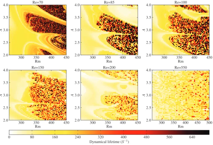
To justify our interest in cycles, we then attempted to check whether the conclusion of Riols et al. (2013), that chaotic dy-namo action at Re = 70 results from their global bifurcations, extends to larger Re. The simplest signature of this effect is in the form of fractal-like sets of initial perturbations for which the dy-namics is long-lived. To check this, we performed several series of DNS spanning a range of Rm and initial conditions, each of them generated from a unique noise realization (using the same procedure as in Sect.3.1) and varying the perturbation amplitude A. We constructed maps of the dynamical lifetimes for each run as a function of Rm and A, for Re = (70, 85, 100, 150, 200, 550). Figure2shows that the boundary separating the regions in phase space where the dynamics is long-lived from those where perturbations decay rapidly has the same qualitative fractal-like structure for all Re. Long-lived simulations are characterized by recurrent dynamics reminiscent of nonlinear cycles, suggesting that the excitation of the MRI dynamo is indeed tied to that of cycles.
At the largest Re considered though, the fractal-like features appear to be smoothed out, and the correspondence between re-current dynamics and chaotic flows less pronounced. We also note that at Re = 550, the transition border seems to be at higher Rm than at Re = 70, in line with the results of Fromang et al.
(2007) and the results of Sect.3.1.
Overall, the previous results suggest that the excitation of self-sustaining MHD turbulence in this problem is related to the existence of MRI dynamo cycles and their global bifurcations. This vindicates the idea that studying how the dynamics of sim-ple nonlinear cycles is affected by changes in Re and Rm may be useful to identify the physical mechanisms responsible for the Pm-dependence of the transition.
4. Parametric study of MRI dynamo cycles
4.1. Existence boundaries in the (Re, Rm) plane
Motivated by the previous results, we investigated the domains of existence in parameter space of three pairs of cycles S N1,
S N2, and S N3 born out of saddle node bifurcations at
pair-specific critical Rmc(Re). S N1 and S N2 have already been
doc-umented byRiols et al.(2013) (see their Figs. 7, 8), while S N3
was found more recently.
Continuation with respect to Re at fixed Rm of the lower and upper branches LB1 and U B1 of S N1 (Fig.3, inset) shows that
they only exist in a finite range of Re, whose extent widens as Rm increases. S N2and S N3 behave similarly (not shown). The
existence boundaries of all cycle pairs in the (Re,Rm) plane were constructed by combining all critical Rmc(Re) and Rec(Rm)
ob-tained by continuation (Fig.3). For Rm in the 300−500 range, all cycles disappear at low enough Pm and their Rmcincreases with
Re. This behaviour, reminiscent of the results ofFromang et al.
(2007), is investigated below (the seemingly large differences between their transitional Re, Rm and ours are essentially due to aspect ratio differences and do not reflect fundamental physical
300 350 400 450 Rm 2.0 2.5 3.0 3.5 4.0 A Re=70 300 350 400 450 Rm 2.0 2.5 3.0 3.5 4.0 A Re=85 300 350 400 450 Rm 2.0 2.5 3.0 3.5 4.0 A Re=100 300 350 400 450 Rm 2.0 2.5 3.0 3.5 4.0 A Re=150 300 350 400 450 Rm 2.0 2.5 3.0 3.5 4.0 A Re=200 300 350 400 450 500 Rm 2.0 2.5 3.0 3.5 4.0 A Re=550 0 80 160 240 320 400 480 560 640 Dynamical lifetime (S−1)
Fig. 2.Maps of dynamical lifetimes as a function of Rm and initial perturbation amplitude A, for a fixed noise realization (see text) and six different Re. The resolution is (δA = 0.04, δRm = 2) except for Re = 70 where (δA = 0.02, δRm = 1) and for Re = 550 where δRm = 5.
0 200 400 600 800 1000 1200 1400 Re 300 350 400 450 500 550 600 R m Pm=1 Pm=0.5 SN1 SN2 SN3 0 100 200 300 400 500 600 Re 0 .4 0 .6 0.8 1.0 1 .2 1 .4 1 .6 1 .8 m a x B0 y U B1 LB1 Rm=352 Rm=390
Fig. 3.Existence boundaries of three cycle pairs (dashed lines) in the (Re,Rm) plane and critical Rec(Rm), Rmc(Re) of saddle nodes obtained by continuation (symbols). Black arrows indicate the regions in which the cycles exist. For S N1, dark blue/black bullets correspond to low resolution results (24×12×36), and light blue/grey bullets are for double resolution (48 × 24 × 72). Inset: selected continuation curves of S N1at fixed Rm.
differences). For S N1, we plotted the critical points obtained for
both low resolution simulations (24 × 12 × 36) and at higher res-olution (48 × 24 × 72). The boundary appears to be almost inde-pendent of resolution. Note that we found it very difficult to ex-plore the strongly nonlinear regime Rm > 500 at the maximum resolution considered. Tentative results at this resolution (not
shown) suggest that SN1 may have an upper boundary in Rm
in this regime.
4.2. Magnetic energy budgets of MRI dynamo cycles
As the MRI dynamo rests on the sustainment of the axisym-metric MRI-supporting field B0 against dissipative processes
through nonlinear interactions of non-axisymmetric modes, analysing the magnetic energy budget of dynamo cycles, most importantly transitional lower branch saddles such as LB1, may
give useful physical insights into the Pm ≤ 1 regime. To do this, we write B = B0+ b1+ X j>2 bj and u = u1+ X j>2 uj, (4)
where u1and b1stand for non-axisymmetric “MRI wave”
per-turbations supported by shearing waves with wavenumbers |ky| =
ky0=2π/Ly, kx(t) = S kyt, |kz| = kz0for u1and kz=0 for b1.
The sum over j ≥ 2 stands for all other (smaller-scale) fluctuations.
We first integrate the energy equation for B0(z, t) over the
volume and half cycle period T/2 = S−1Ly/Lx. Denoting this
operation by hi and taking into account that cyclic magnetic reversals change B0 into −B0, we obtain the energy budget
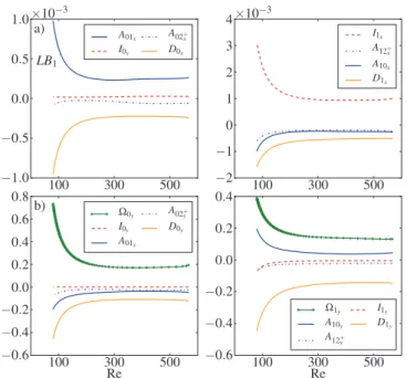
100 300 500 −2 −1 0 1 2 3 4 ×10⁻³ I1x A12+ x A10x D1x 100 300 500 −1.0 −0.5 0 .0 0 .5 1 .0 × 10−3 a) LB1 A01x I0x A02+ x D0x 100 300 500 Re −0.6 −0.4 −0.2 0 .0 0 .2 0 .4 Ω1y A10y A12+ y I1y D1y 100 300 500 Re −0.6 −0.4 −0.2 0 .0 0 .2 0 .4 0 .6 0 .8b) Ω0y I0y A01y A02+ y D0y
Fig. 4.Magnetic energy budgets as a function of Re: a) x projection of
the budgets for B0(left) and b1(right) for LB1at Rm = 390, b) corre-sponding y projection. for B0, Ω0+ I0+ A0+ D0=0, where (5) Ω0 = −S hB0yB0xi ey, I0= hB0◦ B · ∇ui, (6) D0= −η k2 z0hB0◦ B0i, A0= A01+ A02+, (7) A01= −hB0◦ u1· ∇ b1i, A02+= −hB0◦ u · ∇ Bi − A01, (8) and ◦ is the Hadamard (entrywise) product; Ω0 is the energy
provided by the linear stretching of B0x by the shear (Ω effect)
and I0is a nonlinear induction term; A0 is the magnetic energy
exchanged with other modes through nonlinear advection and D0 is the ohmic dissipation; A01 is the energy exchanged with the MRI-unstable waves and A02+is the energy exchanged with
all j ≥ 2 modes. Figure4a,b (left) display the x and y projections of Eq. (5) for LB1as a function of Re, at fixed Rm (U B1is more
energetic but behaves similarly). The MRI-supporting azimuthal field B0y loses energy through laminar dissipation D0y, but also
through a nonlinear advective transfer to other modes A0y < 0,
which therefore acts as a weakly nonlinear (“turbulent”) diffu-sion. The Ω effect is the only net source term for B0y, therefore
the sustainment of B0xis critical for the dynamo. Figure4a (left)
shows that B0x gains energy from the nonlinear term A01x > 0,
which is the product of the MRI correlation of u1 and b1, and
loses energy via D0x and A02+x < 0, so that A01x ≃ |D0x + A02+x|.
A02+
x transfers energy to smaller scales (where it is dissipated),
and can again be interpreted as a nonlinear diffusion of B0x.
To understand how energy is injected into the MRI wave and transferred to B0, we now consider the energy budget for b1,
Ω1+ I1+ A1+ D1= hb1◦(∂ b1/∂t)i ≃ 0, where (9) Ω1 = −S hb1yb1xi ey, I1= I1L+ I1NL, (10) D1= −η h(kx(t)2+ k2y 0) b1◦ b1i, A1= A10+ A12+, (11) 50 150 250 350 450 550 Re 0 .20 0 .25 0 .30 0 .35 |D tx |/ (I0 x + I1x ) U B 1 LB1 Rm=390 Rm=352
Fig. 5.Ratio between nonlinear dissipation Dtxand injected energy I0x+
I1xfor LB1and U B1and two different Rm.
I1L = hb1◦(B0· ∇u1)i and I1NLis a nonlinear induction term; A10 = − A01 = −hb1 ◦ (u1· ∇ B0)i is the energy exchanged
through advection between the MRI wave and B0, and A12+
ac-counts for a similar exchange with smaller scales (Eq. (9) is al-most zero because the wave carries a negligible amount of en-ergy at both t = 0 and t = T/2). Figure4a,b (right) shows that the x and y components of the MRI perturbation b1 are fed by
induction (respectively by I1x and Ω1y, with I1NLx ≪ I1Lx). As
expected, some of the energy injected via the MRI is transferred back nonlinearly to B0x through A10x = −A01x, and some of it is
lost through laminar dissipation D1x. The rest A12+x < 0 is
trans-ferred to smaller scales and can be regarded as a nonlinear diffu-sion of MRI-unstable perturbations. Using a similar analysis, we checked that j ≥ 2 perturbations are mostly excited via nonlin-ear interactions, and not by the MRI, for all cases studied here. Summing Eqs. (5) and (9) to eliminate A01x, we obtain
I0x+ I1x ≃ |D0x+ D1x| + |Dtx|, (12)
which translates that the energy injected via the MRI as I1xmust
balance the total of “laminar” ohmic dissipation |D0x+ D1x|and
nonlinear dissipation |Dtx| ≡ |A12+x + A02+x|for the dynamo to be
sustained (I0x ≪ I1x in all cases studied here).
To understand how Eq. (12) is satisfied in different regimes, we show in Fig.5the ratio |Dtx|/(I0x+ I1x) for LB1and U B1as a
function of Re, for two values of Rm. This ratio is always signif-icantly larger for U B1than for LB1, which is consistent with the
standard picture of upper branches being more nonlinear than lower branches. The amplitude of B0 is larger on U B1 (Fig.3,
inset), which results in a stronger MRI driving (the MRI is al-ways in the regime ky0B0y< Ω here, so the stronger the field, the
larger the growth rate). The most important observation, how-ever, is the significant increase of |Dtx|/(I0x+ I1x) with Re for the
saddle solution LB1, which shows that a larger fraction of the
en-ergy injected in B0and b1is lost through nonlinear dissipation
Dtx = A12+x + A02+x as Re increases. Our interpretation is that this
relative enhancement of “turbulent” magnetic diffusion is tied to the facilitated excitation of velocity fluctuations at large Re.
50 550 0 .4 0 .6 0 .8 1 .0 1 .2 1 .4 ˆ B0 Rm=280 50 550 0 .0 0 .2 0 .4 0 .6 0 .8 1 .0 1 .2 1 |D0x+D1x+Dtx| I0x+I1x |D0x+D1x| I0x+I1x |Dtx| I0x+I1x 50 550 1050 0 .4 0 .6 0 .8 1 .0 1 .2 1 .4 ˆ B0 Rm=350 50 550 1050 0 .0 0 .2 0 .4 0 .6 0 .8 1 .0 1 .2 50 550 1050 1550 2050 Re 0 .4 0 .6 0 .8 1 .0 1 .2 1 .4 ˆ B0 Rm=400 50 550 1050 1550 2050 Re 0 .0 0 .2 0 .4 0 .6 0 .8 1 .0 1 .2 −0.002 0 .000 0 .002 0 .004 ∆Em
Fig. 6. Energy budget of simulations integrated over St = Ly/Lx for three values of Rm. Left: net energy gain ∆Emas a function of Re and
ˆ
B0. ∆Em=0 isolines are shown in black, bullets mark the points ∆Em= 0 for ˆB0 ≃ 0.52. Right: normalized injection and dissipation terms in Eq. (12), as a function of Re, for the same ˆB0.
5. Disappearance of the dynamo
The previous results provide qualitative clues to understand the conditions of excitation of the dynamo. We note that the ampli-tude of B0on LB1seems to asymptote to a constant at large Re
and fixed Rm (Fig. 3(inset)), and therefore so should the MRI growth rate for this branch. This suggests that the MRI may not be able to sustain B0, b1 and therefore the dynamo against the
total effective magnetic diffusion beyond some critical Re, as observed in Figs.3and5. To investigate more precisely how the energy balance of Eq. (12) may be broken, we prepared a fam-ily of initial conditions resembling LB1 at t = 0, consisting of
an axisymmetric field B0 = ˆB0(0.04 ex+ ey) parametrized by
ˆ
B0, plus non-axisymmetric perturbations in the form of a given
packet of shearing waves (|ky| = ky0, kx(t = 0) = 0 and multiple
kz) with weak but random amplitudes (B0x/B0y = 0.04 is
repre-sentative of LB1and ensures that Ω0yis of the order of D0y). This
set of initial conditions was then integrated by DNS during half a cycle period typical of a reversal of B0, for a range of Re and
ˆ
B0. The results were used to construct a map of the net energy
∆Em = I0x + I1x − |D0x + D1x+ Dtx|gained or lost by the active
magnetic modes during the reversal, as a function of Re and ˆB0,
for several Rm (Fig.6(left)). The isolines ∆Em=0 are
reminis-cent of the continuation curves of S N1(Fig.3(inset)). The range
of Re in which the system gains more energy from the MRI than it dissipates (∆Em> 0) widens significantly at larger Rm.
Figure6(right) shows plots of the different terms in Eq. (12) normalized by (I0x + I1x) as a function of Re, for ˆB0 ≃ 0.52.
At Rm = 280, the system loses energy for all Re after a rever-sal. At Rm = 350, there is a range of Re in which more energy is pumped in by the MRI than dissipated. This range widens at even larger Rm = 400. The transition from a sustained to a de-caying regime at large Re occurs because |D0x+ D1x|/(I0x + I1x)
tends to a constant at large Re, while |Dtx|/(I0x + I1x) increases
slowly. The reason why the dynamo can be sustained at larger Re as Rm increases is that the MRI growth rate is not asymptotic in
Rm in the transitional 300−500 Rm range. Laminar dissipation is reduced relative to energy injection as Rm increases, which partially offsets the increase in “turbulent” diffusion at large Re. Equivalently, we may conclude that this increase at large Re re-quires to go to larger Rm to recover the dynamo, as observed in Figs.2and3and reported byFromang et al.(2007).
6. Discussion
Why is the MRI dynamo in Keplerian flow harder to excite at low Pm? Using a simple numerical setup, we have found that weakly nonlinear “turbulent” diffusion (in a qualitative, not strictly mean-field theoretical sense) of large-scale magnetic modes makes it increasingly difficult to sustain the dynamo at moderate Rm as Re increases. The significant advective transfers of magnetic energy to small scales reported byFromang et al.
(2007) in smaller aspect ratio simulations at large Re corroborate this conclusion. A subtle point is that the velocity fluctuations behind turbulent magnetic diffusion in this subcritical problem are not externally prescribed but are indirectly transiently ex-cited by the MRI.
Turbulent diffusion has also been measured in turbulent flows of low Pm liquid metals (Frick et al. 2010;Rahbarnia et al. 2012), in which it is strongly suspected of raising (kinematic) dynamo thresholds (Miralles et al. 2013). Given the very generic nature of this effect, we therefore argue that it could be an impor-tant determinant of MRI dynamo excitation in low Pm rotating shear flows, such as occur in parts of some accretion disks (some of which also have low Rm). Besides, the fact that it also affects MRI-active modes suggests that it may be linked to the drop in angular momentum transport reported in net-flux (imposed field) MRI simulations at (moderately) low Pm.
More work is clearly required to connect these results to the full diversity of simulated and astrophysical regimes, most im-portantly the numerically challenging limit Re ≫ Rm ≫ 1, and to study to which extent the conclusions pertain to numer-ical configurations with different aspect ratio. A similar pre-liminary study in smaller aspect ratio boxes suggests that the same qualitative conclusions apply in this case. These results will be presented in a future paper. Other nonlinear effects, some of which may qualitatively relate to the mean-field theoretical α effect with vertical stratification, are also probably very im-portant in the disk dynamo problem (Brandenburg et al. 1995;
Gressel 2010;Davis et al. 2010;Käpylä & Korpi 2011;Oishi & Mac Low 2011;Simon et al. 2011;Blackman 2012) and will be worthwhile of investigation along the same lines.
Acknowledgements. This research was supported by the University Paul
Sabatier of Toulouse under an AO3 grant, by the Midi-Pyrénées region and by the French National Program for Stellar Physics (PNPS). Numerical calcula-tions were carried out on the CALMIP platform (CICT, University of Toulouse), whose assistance is gratefully acknowledged.
References
Balbus, S. A., & Hawley, J. F. 1991, ApJ, 376, 214 Balbus, S. A., & Hawley, J. F. 1998, Rev. Mod. Phys., 70, 1 Balbus, S. A., & Henri, P. 2008, ApJ, 674, 408
Blackman, E. G. 2012, Phys. Scr., 86, 058202
Bodo, G., Cattaneo, F., Ferrari, A., Mignone, A., & Rossi, P. 2011, ApJ, 739, 82 Brandenburg, A., Nordlund, A., Stein, R. F., & Torkelsson, U. 1995, ApJ, 446,
741
Davis, S. W., Stone, J. M., & Pessah, M. E. 2010, ApJ, 713, 52
Donati, J.-F., Paletou, F., Bouvier, J., & Ferreira, J. 2005, Nature, 438, 466 Frick, P. A., Noskov, V. I., Denisov, S. A., & Stepanov, V. A. 2010, Phys. Rev.
Lett., 105, 184502
Fromang, S., Papaloizou, J., Lesur, G., & Heinemann, T. 2007, A&A, 476, 1123 Goldreich, P., & Lynden-Bell, D. 1965, MNRAS, 130, 125
Gressel, O. 2010, MNRAS, 405, 41
Hawley, J. F., Gammie, C. F., & Balbus, S. A. 1995, ApJ, 440, 742 Hawley, J. F., Gammie, C. F., & Balbus, S. A. 1996, ApJ, 464, 690 Herault, J., Rincon, F., Cossu, C., et al. 2011, Phys. Rev. E, 84, 036321 Käpylä, P. J., & Korpi, M. J. 2011, MNRAS, 413, 901
Lesur, G., & Longaretti, P.-Y. 2007, MNRAS, 378, 1471 Lesur, G., & Ogilvie, G. I. 2008, A&A, 488, 451
Miralles, S., Bonnefoy, N., Bourgoin, M., et al. 2013, Phys. Rev. E, 88, 013002 Oishi, J. S., & Mac Low, M.-M. 2011, ApJ, 740, 18
Rahbarnia, K., Brown, B. P., Clark, M. M., et al. 2012, ApJ, 759, 80
Rincon, F., Ogilvie, G. I., & Proctor, M. R. E. 2007, Phys. Rev. Lett., 98, 254502 Rincon, F., Ogilvie, G. I., Proctor, M. R. E., & Cossu, C. 2008, Astron. Nachr.,
329, 750
Riols, A., Rincon, F., Cossu, C., et al. 2013, J. Fluid Mech., 731, 1 Simon, J. B., Hawley, J. F., & Beckwith, K. 2011, ApJ, 730, 94 Velikhov, E. P. 1959, Sov. Phys. JETP, 36, 1398