A Lagrangian VOF tensorial penalty method for the DNS of resolved particle-laden flows

Open Archive TOULOUSE Archive Ouverte (OATAO)

OATAO is an open access repository that collects the work of Toulouse researchers and

makes it freely available over the web where possible.

This is an author-deposited version published in :

http://oatao.univ-toulouse.fr/

Eprints ID : 11778

To link to this article : DOI:10.1016/j.jcp.2013.08.023

URL :

http://dx.doi.org/10.1016/j.jcp.2013.08.023

To cite this version : Vincent, Stéphane and Brändle de Motta, Jorge

César and Sarthou, Arthur and Estivalezes, Jean-Luc and Simonin,

Olivier and Climent, Eric A Lagrangian VOF tensorial penalty

method for the DNS of resolved particle-laden flows. (2014) Journal of

Computational Physics, vol. 256 . pp. 582-614. ISSN 0021-9991

Any correspondance concerning this service should be sent to the repository

administrator:

[email protected]

A Lagrangian VOF tensorial penalty method for the DNS of

resolved particle-laden flows

Stéphane Vincent

a

,

∗

_{, Jorge César Brändle de Motta}

b

,

c

_{, Arthur Sarthou}

a

,

c

_,

Jean-Luc Estivalezes

b

,

c

, Olivier Simonin

c

, Eric Climent

c

a_{Université de Bordeaux, Institut de Mécanique et Ingénierie (I2M) – UMR 5295, F-33400 Talence, France} b_{ONERA, The French Aerospace Lab, 2, avenue Edouard Belin, 31055 Toulouse, France}

c_{Université de Toulouse, Institut de Mécanique des Fluides de Toulouse, IMFT, UMR 5502, Allée Camille Soula, 31400 Toulouse, France}

a b s t r a c t

Keywords:

DNS of particle flows Resolved scale particles Viscous penalty method Lagrangian VOF Fluidized beds

Collision and lubrication models

The direct numerical simulation of particle flows is investigated by a Lagrangian VOF approach and penalty methods of second order convergence in space for incompressible flows interacting with resolved particles on a fixed structured grid. A specific Eulerian volume of fluid method is developed with a Lagrangian tracking of the phase function while the solid and divergence free constraints are ensured implicitly in the motion equations thanks to fictitious domains formulations, adaptive augmented Lagrangian approaches and viscous penalty methods. A specific strategy for handling particle collisions and lubrication effects is also presented. Various dilute particle laden flows are considered for validating the models and numerical methods. Convergence studies are proposed for estimating the time and space convergence orders of the global DNS approach. Finally, two dense particle laden flows are simulated, namely the flow across a fixed array of cylinders and the fluidization of 2133 particles in a vertical pipe. The numerical solutions are compared to existing theoretical and experimental results with success.

1. Introduction

Interactions between solid particles and a surrounding viscous fluid occurs in many environmental and industrial appli-cations such as combustion devices[1], oil cracking[2], fluidized beds in coal stations and nuclear reactors[3], erosion of sediments on beaches[4]or hygiene and safety[5]. In all these applications, the interaction between the particles and the fluid flow is associated to unsteadiness or turbulence in a complex and not yet well understood manner concerning the drag laws of particles[6]or wall laws of the particulate flow as soon as the particle density is significant. On the one hand, leading simulations at the reactor scale for fluidized beds or combustion chambers require the implementation of macro-scopic Eulerian–Eulerian models [7,8] in which a separation scale is assumed between the particle and the flow scales. These models require drag laws and wall boundary conditions for the flow and the particles which are not yet well posed for dense particle flows. On the other hand, the Direct Numerical Simulation (DNS) of resolved particle flows, for which the grid size is smaller than the particle diameter, are generally restricted to academic configurations including a maximum of thousand of particles. The present work aims at presenting a numerical modeling strategy for the DNS of dense particle flows, validated on various physical test cases including particle–particle and particle–wall interactions or particle settling as well as numerical convergence studies. This DNS particle flow solver will be devoted to simulating the interaction be-tween unsteady or turbulent flows and dense whole of particles to understand the particle response to turbulent flows and

*

Corresponding author.

the modification of turbulence due to the presence of the particles[9]. The DNS tool will allow to extract Lagrangian and Eulerian quantities such as the Lagrangian time scale of the particles, their drag laws or the autodiffusion coefficients[10].

Simulating unsteady particle-laden flows where particle and fluid have the same characteristic scales, i.e. resolved scale particle flows, is the scope of the present work. The Direct Point Simulation (DPS) approaches based on a Lagrangian modeling of the particles does not remain valid for that purpose[11–13]. The field of numerical methods devoted to the simulation of particulate flows involving finite size particles was widely developed the last 20 years concerning the study of the flow over a small number of fixed or moving particle[14–19]or a fixed arrangement of spheres[20]. All the previously mentioned works were developed on fixed grids. The unstructured Arbitrary Eulerian–Lagrangian (ALE) grid simulations were developed for particle flows in the 90’s by Hu et al.[14] concerning two-dimensional flows involving two particles. The works of Maury[21]with the ALE method are also to be noticed concerning the flow of 1000 non-spherical particles in a two-dimensional biperiodic domain. With the same type of approach, two-dimensional ALE simulations of particle motions involving 320 cylinders in a channel have been studied by Cho et al.[22]. However, few of the existing research works have been extended to the simulation of particle flows involving thousand of particles in three dimensions. The work of Hu et al. concerning three-dimensional ALE simulations of the segregation of 90 particles in a vertical channel are among the most advanced results with adapted unstructured grids[23]. A majority of the particulate flow simulations were carried out on structured grids to avoid the complexity of managing an evolving adapted mesh. Among them, the most relevant existing works concern the distributed Lagrangian multiplier (DLM) method of Glowinski and co-workers[24], the Physalis CFD code of Zhang and Prosperetti [25], the Immersed Boundary (IB) with direct forcing approach proposed by Uhlmann

[26,27], the lattice Boltzmann scheme[28,29], the modified version of Uhlmann IB method published by Lucci et al.[30,31]

and the viscous penalty techniques of Ritz and Caltagirone[32]and Randrianarivelo et al.[33,34].

To begin with, the DLM method[24] uses a variational formulation of the Navier–Stokes equations on a fixed grid and the Newton–Euler equations in the solid medium to model the particulate flow. On the interface between the particles and the fluid, Lagrange multipliers are integrated in the variational formulation to satisfy the rigid body motion inside the moving bodies. The force resulting from the interaction between particles is treated by an explicit modification of the particle positions after advection in order to avoid particle overlapping. A short range repulsive force is added in the right hand side of the Newton–Euler equations which is decreasing according to the distance between the center of mass of two particles [24]. The DLM method was utilized to simulate with success the fluidization of 1024 spheres in a square shape tank [35]. As for the Physalis approach[25], fixed grids for the flow solving are combined with analytical Stokes solutions in the vicinity of the particles in order to model the fluid–particle interaction. A cage surrounding the particle shape is used to match the flow solutions arising from a finite difference discretization with the spectral solutions of the Stokes flow. In their approach, Zhang and Prosperetti track in a Lagrangian manner the particles which are subjected to hydrodynamic and external forces. The interaction between the particles is not explicitly modeled. They have applied their numerical method to simulate the interaction between a Homogeneous Isotropic Turbulence (HIT) and particles in a periodic cubic box[25]. They have studied the effect of a two-way coupling procedure on the decaying of the turbulent kinetic energy and the mean particle displacement. Their works were restricted to low Taylor-microscale Reynolds number around 29 as their flow simulation grid was 2563_{. The largest particle simulations dealing with turbulent flow at a resolved particle scale have}

been proposed by Uhlmann concerning the sedimentation of 1000 particles in a periodic box on a 5122

_×

_{1024 grid[26]}

and the turbulent interactions inside a vertical particulate channel flow [27] on a 2048

×

513

×

1024 grid. The numerical methods developed in these works are based on the addition of a direct forcing in the momentum equations to account of the particle presence. The particles are tracked in a Lagrangian manner and the forcing term is also estimated with a Lagrangian approach at the center of the particles. It is redistributed as an Eulerian force thanks to kernel or discrete Dirac functions, according to Peskin work [36]. The particle interaction is treated by means of the repulsive force introduced by Glowinski [24]. A modified version of the IB method of Uhlmann has been proposed by Lucci et al. [30,31] to perform finite sized particle simulations. On a numerical point of view, their modifications concerned the time integration of the Navier–Stokes equations and the management of the two-way coupling force applied on the particles. Lucci and co-workers have investigated the modulation of a HIT flow by particles laying in the range 16 to 35 times the Kolmogorov scale at various Stokes numbers for Taylor-microscale Reynolds numbers of 75 and 110 respectively on 2563 _{and 512}3 _grids.

Parametric studies on the density ratios between particles and fluid with a volume fraction in the range 0

.

01 to 0

.

1 have demonstrated for example that the turbulent kinetic energy was reduced by the particles compared to a reference single phase HIT flow. A different finite-size particle modeling has been proposed by Ten Cate et al. [28] which is related to lattice Boltzmann approaches. In their approach, the interaction between particles and fluid and the so the no-slip solid boundary condition is enforced through a body force added to the momentum equations. This force accounts for lubrication and repulsive effects during particle interactions. With the lattice Boltzmann model, Ten Cate and co-workers have studied the energy spectra and particle distribution functions for particles placed in a forced homogeneous turbulence for various Stokes numbers at a Taylor microscale Re

=

61 on a 2563 _{grid. Other authors have used a classical bounce-back technique}

for simulating the sedimentation of turbulent particle-laden flows[29]. To finish with, a wide literature has been devoted to the numerical modeling of finite size particle flows by means of fictitious domains and penalty methods[18,32,33,37]. The penalty techniques consist in playing on the magnitude of the dynamic viscosity to impose the local solid character of the medium. In recent works, an Implicit Tensorial Penalty Method (ITPM), based on a decomposition of the viscous stress tensor, has been proposed to deal with particulate flows with an accuracy between 1 and 2 in space convergence[38–40]. The ITPM has been applied to the DNS of fluidized beds containing 2133 particles by Corre et al.[10].

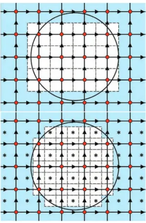
Fig. 1. Definition sketch of the fictitious domain approach for a finite size particulate flow. The underlaying grid, the phase function C and the fluid–particle

interfaceΣare plotted.

The present work proposes a second order in space penalty method for the DNS of particulate flows based on the ITPM. The objective is to build an as implicit as possible approach in which the particle positions are not modified after tracking with the single fluid velocity obtained on structured Cartesian mesh, even in the case where particle collisions are present. The penalty method is chosen, instead of the DLM or direct forcing approaches, for its fully coupled character, robustness and easy implementation, as it is based on the existing physical terms in the momentum conservation equations. In addition, Lagrangian VOF approaches are implemented and the single fluid formulation of Kataoka[41]is extended to the framework of fluid–solid particle interactions. The whole algorithms are parallelized with MPI instructions for dealing with large grid simulations.

The article is organized as follows. In the first part, the models and numerical methods are detailed paying attention to describing the original part of the numerical algorithms. In particular, a mixed Lagrangian–Eulerian VOF technique is used to follow the particle during time and an implicit treatment of the particle to particle or particle to wall interaction is implemented. An augmented Lagrangian approach and viscous penalty techniques are also proposed for dealing with the velocity-pressure coupling and the solid body motion. All these features are extended to parallel computations. The third section is devoted to numerical convergence exercises and physical validations. An application to a fluidized bed in a cylindrical tank is presented in the forth section. Conclusions and perspectives are finally drawn in the last section.

2. A tensorial penalty approach for finite size particulate flows

2.1. Fictitious domain framework

The numerical simulation of a particulate flow interacting with a surrounding fluid can be investigated following two different numerical strategies: unstructured or structured grids. This important choice is motivated by the representation of the complex shape involved by the interface between a fluid and thousand of moving particles. On the one hand, the more natural solution seems to be the implementation of an unstructured body-fitted grid to simulate the fluid area in the two-phase particle flow[14,21–23]. Building such a finite-volume or finite-element mesh in three-dimensions is not easy and requires automatic mesh generators as the solid particles move according to time and space. The remeshing process at each calculation step is time consuming and can be very difficult to manage automatically in computer softwares when global shape of the fluid–solid interface is complex[42]. On the other hand, it can be imagined to develop a fixed structured grid to simulate particle flows. In this case, the mesh is not adapted to the fluid–solid interfaces and includes both phases. The difficulty lies in the taking into account of the presence of particles in the fluid whose interface is not explicitly tracked by the non-conforming mesh. This type of modeling and numerical problem belongs to the class of fictitious domains[24, 43]. The modeling strategy developed hereafter is based on this approach.

Instead of solving two sets of equations, i.e. the classical Navier–Stokes equations in the fluid phase and the Newton–Euler equations in the solid phase, and connecting the solutions at the fluid–solid interface thanks to jump equations, as proposed for example by Delhaye[44]for fluid interfaces or by Maury[21]for particle flows, the fictitious domain method consists in introducing a phase function C to locate each medium and to formulate a global model valid in the fluid and solid parts of the flow. According to the local value of C , the physical characteristics and the conservation equations are adapted to fulfill the correct physical behavior. By definition, C

=

1 in the solid, C

=

0 in the fluid and the interface

Σ

between the fluid and solid phases is associated to the isosurface C

=

0

.

5. A two-dimensional definition sketch is illustrated inFig. 1for the DNS of finite size particle flows.

2.2. Generalized one-fluid model for particulate flows

Incompressible two-phase flows involving a carrier fluid and a solid phase can be modeled by solving the incompressible Navier–Stokes equations together with a phase function C describing the particle phase shape evolutions through an advec-tion equaadvec-tion on the corresponding phase funcadvec-tion. As explained by Kataoka [41,45], the resulting model takes implicitly into account the jump relations at the interface[44,46]and the fluid–solid interface evolutions are taken into accounts in an Eulerian manner by the advection equation on C :

∇ ·

u

=

0 (1)

ρ

µ ∂u

∂

t

+ (u

· ∇)u

¶

= −∇

p

+

ρ

g

+ ∇ ·

¡

µ

¡∇u

+ ∇

tu¢¢ +Fsi (2)

∂

C

∂

t

+

u

· ∇

C

=

0 (3)

where u is the velocity, p the pressure, t the time, g the gravity vector,

ρ

and

µ

respectively the density and the viscosity of the equivalent fluid. Concerning the turbulence modeling, it is assumed that all the space and time scales of the flow are solved and so that direct numerical simulations are performed with the present particulate one-fluid model. Deterministic Large Eddy Simulation (LES) models could also be used to take into account the under-resolved sub-grid scale turbulence structures [47]. However in this case, a specific attention should be paid in the vicinity of the particle–fluid interface, as specific sub-grid stress tensors arise in these zones [48]. The two-way coupling between particle and fluid motions is ensured in the momentum equations by the presence of a solid interaction force Fsiwhich will be detailed and discussed in

the following Section2.5. This interaction force will be activated as soon as a collision between two particles or a particle and a wall will occur.

The one-fluid model is almost identical to the classical incompressible Navier–Stokes equations, except that the local properties of the equivalent fluid (

ρ

and

µ

) depends on C , the interface localization requires the solving of an additional equation on C . A specific volume force is added at the interface to account for particle collision effects. Satisfying the solid constraint in the particles requires to develop a specific model. A penalty approach on the viscosity is proposed and detailed in the next section.

2.3. Penalty methods for solid behavior and incompressibility 2.3.1. Second order implicit tensorial penalty method

As explained in the previous sections, the one-fluid model and the fictitious domain approach formulated for dealing with particle flows require to consider each different phase (fluid, solid) as a fluid domain with specific rheological property. Each sub-domain is located by a phase function C . Ensuring the solid behavior in the solid zones where C

=

1 requires to define a specific rheological law for the rigid fluid without penalizing the velocity, as the particle velocities are not known

a priori in the problems considered here (particle sedimentation, fluidized beds, turbulence particle interaction).

A specific model is designed for handling the solid particle behavior in the one-fluid Navier–Stokes equations. It is based on a decomposition of the stress tensor

σ

, which reads for a Newtonian fluid (see[49]and[50]):

σ

i j

= −

p

δ

i j

+ λ∇ ·

uδi j

+

2

µ

Di j (4)

where

λ

et

µ

are respectively the compression and shearing viscosities and D is the tensor of deformation rate.

Following the work of Caltagirone and Vincent [51], the stress tensor can be reformulated so as to distinguish several natural contributions of the stress tensor dealing with compression, tearing, shearing and rotation. The interest of this decomposition is then to allow a distinct penalization of each term in order to strongly impose the associated stress. If we assume that the Navier–Stokes equations for a Newtonian fluid contain all physical contributions traducing compressibility effects, shearing or rotation, their splitting allows to act differentially on these effects by modifying the orders of magnitude of each term, through the related viscosity coefficients, directly in the motion equations.

Decomposing

σ

i j according to the partial derivative of the velocity in Cartesian coordinates, we obtain[51]

σ

=





−

p

+ λ∇ ·

u 0 0 0

−

p

+ λ∇ ·

u 0 0 0

−

p

+ λ∇ ·

u





+

κ







∂u ∂x 0 0 0 ∂v ∂y 0 0 0 ∂w ∂z







+ ζ







0 ∂u ∂y ∂u ∂z ∂v ∂x 0 ∂v ∂z ∂w ∂x ∂w ∂y 0







−

η







0 ∂u ∂y

−

∂v ∂x ∂u ∂z

−

∂w ∂x ∂v ∂x

−

∂u ∂y 0 ∂v ∂z

−

∂w ∂y ∂w ∂x

−

∂u ∂z ∂w ∂y

−

∂v ∂z 0







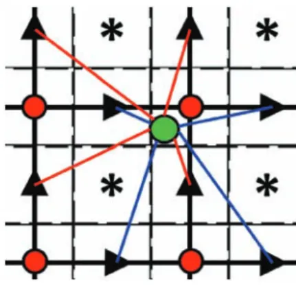
(5)

Fig. 2. Discrete interpretation of the direct viscous penalty method (top) and split viscous penalty approach (bottom) on staggered grids – the pressure

points are plotted in red circles, the velocities as arrows and the pure shearing and rotations viscosities as stars. The black line represents the interface between a particle and the carrier fluid.

This decomposition of the stress tensor in which new viscosity coefficients appear artificially is written in compact form as

σ

i j

= (−

p

+ λ∇ ·

u)δi j

+

κ

Λ

i j

+ ζ Θ

i j

−

η

Γ

i j (6)

where

λ

is the compression viscosity,

κ

is the tearing viscosity,

ζ

is the shearing viscosity and

η

is the rotation viscosity. The usual form of

σ

is easily recovered by stating

λ

= −

2

/

3

µ

,

κ

=

2

µ

,

ζ

=

2

µ

and

η

=

µ

. As only incompressible particle flow configurations will be considered here,

λ

will be taken equal to zero. Finally, the divergence of the viscous stress tensor for a Newtonian fluid appearing in the one-fluid model(2)reads

∇ ·

¡

µ

¡∇u

+ ∇

tu¢¢ = ∇ · £

κ

Λ(u)¤ + ∇ · £ζ Θ(u)¤ − ∇ · £

η

Γ (u)

¤

(7)

The main interest of the formulation (7) is to dissociate stresses operating in a viscous flow and then to make the implementation of a numerical penalty method easier. The use of the viscosities

κ

,

ζ

and

η

allows to impose a solid behavior in the zones where C

=

1 by stating for example

η

≫

1,

κ

=

2

η

and

ζ

=

2

η

in these zones. In this case, it is imposed that the local solid flow admits no shearing, no tearing and a constant rotation according to the surrounding flow constraints. These flow constraints are implicitly transmitted to the particle sub-domain as they are solved with the fluid motion at the same time. The previous viscous penalty method is formally equivalent to choosing

µ

≫

1 to impose a solid behavior. However, on a discrete point of view, the two formulations are not equivalent. Indeed, on a staggered grid, the elongation viscosity is located on the pressure nodes whereas the pure shearing and rotation viscosities lie on a specific grid, at the center of the mesh grid cells, as illustrated inFig. 2. If the dynamic viscosity

µ

is used to impose the solid behavior in the zones where C

=

1, a first order convergence in space is obtained as the entire grid cell is assumed solid in this case. A rasterization effect is in this way produced at the particle–fluid interface

Σ

by the Direct Viscous Penalty technique (DVP). When the viscous stress tensor splitting(7)is used to impose the solid behavior, the belonging of each viscosity point to the particle can be considered (elongation viscosity on the pressure points and pure shearing and rotation viscosities on the viscous points). A more accurate accounting of the fluid–solid interface is so involved in this case thanks to the introduction of a dual grid for the pure shearing and rotation viscosities. The rasterization effect is so reduced. A second order convergence in space is obtained with the Split Viscous Penalty (SVP) formulation. These viscous penalty approaches will be discussed and compared in the validation section.

2.3.2. Augmented Lagrangian methods for multi-phase flows

Following a similar walkthrough as in the work on Stokes and Navier–Stokes equations proposed by Fortin and Glowinski

[52], the augmented Lagrangian method can be applied to the unsteady Navier–Stokes equations dedicated to particulate flows. The main objective is to deal with the coupling between the velocity and pressure and to account of fluid and solid constraints. Starting with u∗,0

₌

_un _{and p}∗,0

₌

_pn_{, the standard augmented Lagrangian solution reads}

while

°

°∇ ·

u∗,m

°

°

>

ǫ

,

solve

¡

u∗,0

,

p∗,0

¢ = ¡u

n

_,

_pn

¢

ρ

µ

_u∗,m

₋

_u∗,0

1

t

+

u ∗,m−1

_{· ∇u}

∗,m

¶

_{− ∇}

¡

r

∇ ·

u∗,m

¢ = −∇

p∗,m−1

+

ρ

g

+ ∇ ·

£

µ

¡∇u

∗,m

_{+ ∇}

T_u∗,m

_{¢¤ +}

_F si p∗,m

=

p∗,m−1

−

r

∇ ·

u∗,m (8)

where r is the augmented Lagrangian parameter used to impose the incompressibility constraint, m is an iterative conver-gence index and

ǫ

a numerical threshold controlling the constraint. Usually, a constant value of r is used, for example equal to the average between the minimum and maximum eigenvalues of the linear system for Stokes flows[52]. From numerical experiments, optimal values are found to be of the order of

ρ

iand

µ

iin each phase (fluid or solid) to accurately solve the

motion equations in the related zone[38,39]. The momentum, as well as the continuity equations, are accurately described by the solution

(u

∗

,

p∗

₎

_{coming from(8)in the medium to which the value of r is adapted. However, high values of r in}

the other zones act as penalty terms inducing the numerical solution to satisfy the divergence-free property only. Indeed, if we consider for example

ρ

1

/

ρ

0

=

1000 (characteristic of a solid particle in air) and a constant r

=

ρ

1 to impose the

divergence-free property in the particles, the asymptotic equation system solved is:

ρ

µ

_u∗

₋

_un

1

t

+

¡

un

· ∇

¢

u∗

¶

− ∇

¡

r

∇ ·

u∗

¢ =

ρ

g

− ∇

pn

+ ∇ ·

£

µ

¡∇u

∗

_{+ ∇}

T_u∗

_{¢¤ +}

_F si in

Ω

1 u∗

−

un

1

t

− ∇

¡

r

∇ ·

u∗

¢ =

0 in

Ω

0 (9)

where

Ω

0 and

Ω

1refer respectively to the fluid and solid phases. The idea of locally estimating the augmented Lagrangian

parameter in order to obtain satisfactory equivalent models and solutions in all the media was first developed in[38]and

[39]. Instead of choosing an empirical constant value of r fixed at the beginning of the simulations, and to avoid the main remaining drawback of the adaptive methods published in [38]and[39] which are linked to the a priori definition of di-mensionless parameters for defining r

(

t

,

M

)

, it has been proposed in [53] to define the augmented Lagrangian parameter as an algebraic parameter which increases the magnitude of specific coefficients in the linear system in order to verify the divergence free constraint, while solving at same time the conservation equations. The main interests of the algebraic adaptive augmented Lagrangian method are the following: it does not require any a priori physical information, it applies to any kind of geometry and grid and it takes into account the residual of the linear solver and the fulfillment of incom-pressible and solid constraints. This version of the algebraic adapted augmented Lagrangian (3AL) method will be used in the present work, coupled to viscous penalty methods and particle interaction models. The main interest of the 3AL is that its formulation, as proposed in[53], is directly adapted to the penalization of the viscous stress tensor through the dynamic viscosity penalty or the split viscous penalty as it lies on a scanning of the matrix resulting from the discretization of the penalized conservation equations. The algorithm(8)remains valid for particulate flows with r a function of time and space of the form[53]

r

(

t

)

i

=

K

max

(

Ai j

,

j

=

1

..

N

)

(10)

where i is the index of the discrete velocity solution on a grid containing N velocity points and j the index for the discretization stencil of the equation for a given ith velocity unknown. The discretization matrix containing the viscous penalty contributions is referred to as A, Ai j being the coefficient of A at the line i and the column j. The constant

K

is

used to strengthen the penalization of the divergence free constraint in the momentum equations. It is generally chosen between 100 and 1000.

2.3.3. Physical characteristics of the equivalent fluid

The fictitious domain approach used in the present work considers the solid part of the particulate flow as a fluid with specific rheological properties whose evolutions are modeled by the Navier–Stokes equations. The present section explains how the characteristics of the solid equivalent fluid are defined to ensure a deformation free behavior in the related zones.

Classically, for any point P belonging to the solid zones of the calculation domain

Ω

, i.e. the zones where C

=

1, the solid behavior is characterized by a translation and a rotation. For any particle, constant translation and rotation velocities

u0 and w exist such that

where XI

Bis the barycenter of the considered particle I and

Ω

I _{the related solid sub-domain. The solid constraint is}

intrin-sically maintained if the deformation tensor is nullified:

∀P

∈ Ω

I

,

∇u

+ ∇

Tu

=

0 (12)

In other words, if we assume that(12)is satisfied, the following systems are obtained:



























∂

u

∂

x

=

0

∂

v

∂

y

=

0

∂

w

∂

z

=

0 (13)































∂

u

∂

y

= −

∂

v

∂

x

∂

v

∂

z

= −

∂

w

∂

y

∂

w

∂

x

= −

∂

u

∂

z (14)

Then, Eqs.(13)give the direction dependencies of each velocity components as

u

=

u(y

,

z

),

v

=

v(x

,

z

),

w

=

w(x

,

y

)

(15)

By using Eqs.(14), three functions

ω

1

(

x

)

,

ω

2

(

y

)

and

ω

3

(

z

)

can be defined such that































∂

u

(

y

,

z

)

∂

y

= −

∂

v

(

x

,

z

)

∂

x

=

ω3

(

z

)

∂

v

(

x

,

z

)

∂

z

= −

∂

w

(

x

,

y

)

∂

y

=

ω1

(

x

)

∂

w

(

x

,

y

)

∂

x

= −

∂

u

(

y

,

z

)

∂

z

=

ω2

(

y

)

(16)

If it is assumed that the rotation velocity components have the necessary regularity, the Schwarz theorem gives a constant second order derivative of the velocities:



































∂

2u

(

y

,

z

)

∂

y

∂

z

=

∂

ω3

(

z

)

∂

z

= −

∂

ω2

(

y

)

∂

y

=

W1

∂

2v

(

x

,

z

)

∂

x

∂

z

=

∂

ω1

(

x

)

∂

x

= −

∂

ω3

(

z

)

∂

y

=

W2

∂

2w

(

x

,

y

)

∂

x

∂

y

=

∂

ω2

(

y

)

∂

y

= −

∂

ω1

(

x

)

∂

x

=

W3 (17)

It can be verified that the second order derivatives are equal to zero by solving the following system:







W2

= −

W3 W3

= −

W1 W1

= −

W2 (18)

As a consequence, the functions

ω

1,

ω

2 and

ω

3 are constant and therefore continuous and derivable with continuous

derivatives. Finally, by integrating Eqs.(17), we obtain







u

=

u0

+

ω3

y

−

ω2

z v

=

v0

+

ω1

y

−

ω3

z w

=

w0

+

ω2

y

−

ω1

z (19)

Eq.(11) is so verified if(12) is true. In this way, relations (11)and (12)are equivalent. Then, a solid constraint can be solved by computing

∇u

+ ∇

Tu

=

0. For the resolution of the momentum conservation equation(2)in the Navier–Stokes equations, this condition is asymptotically verified when

µ

→ +∞

, as explained in Section2.3.1.

According to the decomposition of the viscous stress tensor introduced in Section2.3.1, an equivalent condition to(11)

Λ(u)

=

0 (20)

Γ (u)

=

2

Θ(u)

(21)

Indeed, it can be verified that

∇

u

+ ∇

Tu

=

2

Λ(u)

+

2

Γ (u)

− Θ(u)

. For any Newtonian fluid or solid media, the relations

κ

=

2

µ

,

ζ

=

2

µ

and

η

=

µ

must be satisfied, as proposed in Section2.3.1, together with

µ

≫

1 in the particles.

Numerically, Eqs.(12),(20)and(21)have to be implemented on the split viscous penalty grid described in Section2.3.1

inFig. 2. For internal solid nodes (those where C

=

1) the solid viscosity is chosen to be 100 to 1000 times the viscosity of the carrier fluid. This choice will be discussed in the validation section concerning the accuracy of the simulations and the effect on the cost of the linear solvers. The previous remarks on the order of magnitude of the viscosity inside the solid parts stand for the continuous point of view.

On a discrete point of view, the flow grid cells cut by the fluid–solid interface

Σ

must be distinguished compared to those entirely included in the particles. For these last nodes, the dynamic viscosity is chosen equal to

µ

∞

≈

K

µ

carrier fluid

with 100

6

K

6

1000. For the fluid–solid cells, different methods can be used to define the homogenized viscosity. First, to avoid any direct interpolation of the viscosity coefficients associated to off diagonal viscous stress tensor components, an interpolation Cµ of the volume fraction is defined at the viscosity nodes, i.e. stars inFig. 2on the split viscous penalty grid:

Cµ

=

1 4

X

N CN (22)

where N denotes the indices of the pressure nodes located at the vertices of the cell to which Cµ belongs. Four different numerical viscous laws have been investigated according to C for the diagonal viscous stress tensor terms, i.e. red circles in

Fig. 2, Cµ and also a conditional indicator function IC satisfying IC<0.5

=

1 if C

<

0

.

5 or IC>0.5

=

1 if C

>

0

.

5:

1. Numerical viscous law 1 (NVL1), the viscosity is defined in a discontinuous way according to Cµ:

κ

=

2

[

µ

fIC<0.5

+

µ

sIC>0.5

]

ζ

=

2

[

µ

fICµ<0.5

+

µ

sICµ>0.5

]

η

=

µ

fICµ<0.5

+

µ

sICµ>0.5

2. Numerical viscous law 2 (NVL2), the viscosity is given by an arithmetic average:

κ

=

2

[(

1

−

C

)

µ

f

+

C

µ

s

]

ζ

=

2

[(

1

−

Cµ

)

µ

f

+

Cµ

µ

s

]

η

= (

1

−

Cµ

)

µ

f

+

Cµ

µ

s

3. Numerical viscous law 3 (NVL3), the viscosity is given by a harmonic average:

κ

=

2

[

µfµs Cµf+(1−C)µs

]

ζ

=

2

[

_C µfµs µµf+(1−Cµ)µs

]

η

=

µfµs Cµµf+(1−Cµ)µs

4. Numerical viscous law 4 (NVL4), the viscosity is defined with a mixed average as proposed by Benkenida and Magnaudet

[54]:

κ

=

2

[(

1

−

C

)

µ

f

+

C

µ

s

]

ζ

=

2

[

_C µfµs µµf+(1−Cµ)µs

]

η

=

µfµs Cµµf+(1−Cµ)µs

Concerning the density, an arithmetic average is used whatever its location on the discretization grid. The most clever choice of viscosity average for the ITPM will be discussed in the validation section.

2.4. Eulerian–Lagrangian VOF method for particle tracking

Once the particle center of mass is known in the computations, it has been explained that the ITPM requires to locate the interior and exterior of the particle thanks to a phase function C in order to build the physical properties of the equivalent fluid such as the dynamic viscosity. This section explains how at each time step the finite size particles are advected and how the solid fraction C is obtained on the Eulerian flow grid.

At each time step, the mass and momentum equations are solved by using the augmented Lagrangian approach explained before including the particle–particle collision forces Fsi detailed in Section2.5. Thanks to the ITPM, the one-fluid velocity

field provides the solid velocity field inside the particles. Then, instead of using a classical Eulerian VOF approach[53,55,56]

to obtain the new solid fractions in each Eulerian cells by solving Eq. (3), the Lagrangian velocities VI,L _{of each particle,}

located in a Lagrangian way by their position XI,L_{, are computed at reference points (the four green points inFig. 3, in the}

two-dimensional configuration) located inside each particle by using an interpolation method explained in Section2.4.1. The new positions of the particles are then updated in a Lagrangian manner, as developed in Section2.4.2 and finally the new Eulerian solid fractions are estimated by means of a projection of the exact shape of the particles on the flow grid. This last step is detailed in Section2.4.3. The interest of using a Lagrangian scheme to advect the particles and to project their shape

Fig. 3. Position in two dimensions of the reference Lagrangian points (green points) used to interpolate the Lagrangian velocity at the barycenter of the

particles. (For interpretation of the references to color in this figure, the reader is referred to the web version of this article.)

Fig. 4. Eulerian velocity kernel (u-components in blue and v-components in red) used in two dimensions to estimate the components of the interpolation

Lagrangian velocity points (green point). (For interpretation of the references to color in this figure, the reader is referred to the web version of this article.)

on the Eulerian mesh is to avoid any distortion of the particle shape over time, as would be induced by a classical Eulerian VOF scheme.

2.4.1. Computation of particle velocity

The Lagrangian particle velocity located at the center of each solid sphere is computed by using 4 or 6 points respectively in two or three dimensions. The same procedure allows to estimate the rotation velocity if required. InFig. 3, the position of the velocity calculation point, colored in green, is represented for the two-dimensional case. These points are positioned on the axis parallel to the Cartesian coordinate system axis, at half the radius of the particles on each side of the center of the spheres. We have observed that it was more accurate to define the Lagrangian velocity of the particles by using fixed points located inside the frame of the particles compared to an Eulerian average of the velocity field inside each solid sphere. A lower accuracy has been also obtained with the use of a kernel based interpolation[57]. With the proposed four or six point approach, the idea is to estimate the Lagrangian velocity VI,L _{at the barycenter of the spheres by interpolating it at}

the X_kI,L locations according to the surrounding Eulerian solid velocity field. Index I stands for the number of the particle and k

=

1

..

N for the number of the interpolation point associated to particle I, with N

=

4 in 2D and N

=

6 in 3D. The velocity is interpolated from the nearest Eulerian velocity node values as shown inFig. 4for the two-dimensional case. The relative positionsX of the interpolation points compared to the Eulerian velocity components X

˜

uand particle center XI,L is

first calculated as

˜

X

=





˜

x

˜

y

˜

z





=

XI_k,L

−

Xu DXI,L (23)

where for a given interpolated Lagrangian velocity component, DXI,L _{refers to the distance vector in each Cartesian}

co-ordinate between two opposite points of the box (parallelepiped in three dimensions) formed by the Eulerian velocity components used for the interpolation. In two dimensions, the surrounding Eulerian components used to interpolate VI_k,L are represented inFig. 4with blue (u-component) and red (v-component) lines joining the Lagrangian interpolation posi-tion XI_k,L.

The basis Pm, m

=

1

..

N of the bilinear interpolation is then built according to the n (n

=

4 in 2D and n

=

8 in 3D)

Eulerian velocity components Vn as follows

P1

=

V1 (24)

P2

=

V2

−

V1 (25)

P3

=

V4

−

V1 (26)

P4

=

V1

+

V3

−

V2

−

V4 (27)

in two dimensions and

P1

=

V1 (28) P2

=

V2

−

V1 (29) P3

=

V4

−

V1 (30) P4

=

V5

−

V1 (31) P5

=

V3

+

V1

−

V2

−

V4 (32) P6

=

V6

+

V1

−

V2

−

V5 (33) P7

=

V8

+

V1

−

V4

−

V5 (34) P8

=

V7

−

V6

−

V8

+

V5 (35)

in three dimensions. The lth component of the Lagrangian interpolated velocity is obtained by

V_kI,_,lL

=

P1

+

P2x

˜

+

P3y

˜

+

P4

˜

xy

˜

in 2D (36)

V_kI,_,lL

=

P1

+

P2x

˜

+

P3y

˜

+

P4

˜

z

+

P5x

˜

˜

y

+

P6x

˜

˜

z

+

P7z

˜

y

˜

+

P8

˜

xy

˜

˜

z in 3D (37)

Finally, the Lagrangian velocity at the barycenter of the particle reads

VI,L

=

P

NVI ,L k N (38)

2.4.2. Transport of the particles

Once the Lagrangian particle velocity is known by(38), the particles are advected in a Lagrangian manner by an update of the position of their mass center XI,L _{as follows}

XI,L,n+1

=

XI,L,n

+ 1

tVI,L,n+1 (39)

with the second order Lagrangian velocity extrapolation at time

(

n

+

1

)1

t being given by

VI,L,n+1

=

V

I,L,n

₊

_VI,L,n+1/2

2 (40)

The intermediate Lagrangian particle velocity is defined according to the interpolated position of the particle I at time

(

n

+

1

/

2

)1

t, which is given by XI,L,n+1/2

₌

_XI,L,n

_{+ 1}

_tVI,L,n_{, as follows}

VI,L,n+1/2

=

P

NV I,L,n+1/2 k N (41)

The Lagrangian particle advection scheme(39)–(41)corresponds to a second order accurate in time Runge–Kutta scheme.

2.4.3. Update of the solid fraction

The one-fluid model used to simulate the particle flow does not explicitly use the Lagrangian positions or velocities of the solid spheres. As a fictitious domain approach, it requires the accounting of the Eulerian solid fraction C in each Eulerian grid cell. The phase function C have to be computed according to the Lagrangian position of particles at time

(

n

+

1

)1

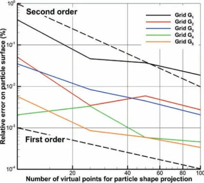
t instead of solving explicitly the Eulerian advection equation on C . This is achieved by generating a set of virtual

test points on a regular network inside each pressure control volume, as described for the two-dimensional case in Fig. 5. On a statistical point of view, the local solid fraction in a given control volume is naturally defined by the number of virtual points belonging to the interior of the particle normalized by the total number of virtual points used in the control volume. The effect of the number of virtual points on the accuracy of the surface of the particle projected on the Eulerian flow grid is proposed inFig. 6. Various Eulerian grids are considered, i.e. G1, G2, G3, G4 and G5, containing respectively 5, 10,

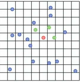
Fig. 5. Two-dimensional network of 10Ndimvirtual points used to estimate the local solid fraction Cn+1_{thanks to a Lagrangian position X}I,L,n+1_{of a particle,}

whose interface is notedΣ. In green are plotted the virtual points belonging to the particle and in blue the other ones. In the example, Cn+1

=92/100= 0.92. (For interpretation of the references to color in this figure, the reader is referred to the web version of this article.)

Fig. 6. Error on the projected surface of a circular shape particle according to the number of virtual points in each space direction and to the Eulerian grid

used.

particle diameter, the relative error on the particle shape is less than 0

.

1%. Increasing the number of virtual points reduces the error on the particle surface, with a convergence order between 1 and 2. The network of virtual points which will be considered in our simulations will be composed of 25Ndim _{points, with Ndim the number of dimensions of the problem.}

Indeed, it can be observed that in this case, the error on the solid fraction estimate is always less than 0

.

1% whatever the computational flow grid. This constraint is important to deal with DNS of particulate flows as only a moderate number of Eulerian cells along a particle diameter can be used in three-dimensional simulations to simulate realistic problems.

2.5. Numerical modeling of particle interaction

Leading fully resolved particulate simulations requires to manage the contact and collisions between particles in order to prevent overlapping between particles or particles and walls. This spurious numerical phenomenon is in particular induced by the approximation of the particle trajectories and the projection of the spherical shape on the Eulerian grid. For volume ratios of particles lower than 0

.

1%, collisions are often assumed negligible [58,59]. As soon as a general particulate flow model is built for low and high solid fractions, the collisions can be a major physical phenomenon, such as in fluidized beds.

The fully resolved numerical simulations have to integrate a collision model to prevent unphysical adhesion of particles and try to represent reality. This point is developed in the present section.

2.5.1. Existing models for particle interaction

A first approach consists in defining a mass-damping force [10,24]or an exponential repulsive force [18] that ensures that particles do not collide. These methods do not include a priori the explicit modeling of the influence of the lubrication effects. Several solutions exist to account for lubrication: the first one is based on a local refinement of the flow grid in order to resolve the lubrication effect [60,61]. Therefore, this approach is very expensive in three dimensions. Another solution consists in adding an equivalent force to the repulsive component in order to reproduce the lubrication force. We have chosen this strategy, based on the work of Breugem[62].

2.5.2. Solid/solid collision

A normal solid/solid collision is characterized by the dry coefficient of restitution (in air), ed, defined as the ratio between

the velocity after and before the collision. The energy absorbed by the collision is represented by the ed coefficient. For a

solid collision between steel spheres, the collision time is around 10−9 _{seconds. This time is too small to be reproduced by}

the fluid simulation with a time step chosen according to macroscopic hydrodynamic effects, with

1

t laying in the range

10−6–10−2s in most of the fluid mechanics problems involving particles such as a fluidized bed or a sedimentation flow. The solution in which a repulsive force is used to prevent from particle numerical adhesion is known as smooth spheres

[63]. The main drawback of this model is that it artificially separate particles or walls as soon as they are distant from one grid cell. In this way, the collision effect is not accurately modeled and the restitution coefficient is generally underestimated. In order to account explicitly for the restitution coefficient, a damping-mass force is used, instead of a standard smooth sphere repulsive force, according to Eq. (42) where Nc

1

t represents the collision time, which is always overestimated.

Preliminary tests have shown that using Nc

=

8 is a good compromise to get a correct collision model (more details on the

numerical implementation are given in[64])

Fs

=

me

(

π

2

+

ln

(

ed

)

2

)

[

Nc

1

t

]

2 d

−

2meln

(

ed

)

[

Nc

1

t

]

˙

d (42)

where me is the reduced mass verifying me

= (

m−1₁

+

m−1₂

)

−1 for inter-particle collision and me

=

m for particle wall

collision, d is the distance vector in each Cartesian direction between the particles or the particle and the wall andd is the

˙

time derivative of d. Notations m1 and m2 stand for the masses of particle 1 and 2 whereas m denotes the mass of the

particle in a particle/wall collision configuration. The restitution coefficient is given by the user depending on the material and particle properties. This input parameter have to be measured experimentally.

2.5.3. Lubrication

Many authors propose models that include the lubrication effects [60,65,66]. The principle consists in utilizing the ana-lytical development given by[67]or the lower order development provided by[63] of the forces exerted by a viscous fluid between two particles or a particle and a wall. The following formulation of the lubrication force is considered here:

Fl

(

ǫ

i

,

un

)

= −

6

π µ

fRun

£λ(

ǫ

i

)

− λ(

ǫ

al

)

¤

(43)

with

λ

being defined for particle–particle interaction as

λ

pp or as

λ

p w for particle–wall interaction

λ

pp

=

1 2

ǫ

i

−

9 20log

(

ǫ

i

)

−

3 56

ǫ

ilog

(

ǫ

i

)

+

1

.

346

+ °(

ǫ

i

)

(44)

λ

p w

=

1

ǫ

i

−

1 5log

(

ǫ

i

)

−

1 21

ǫ

ilog

(

ǫ

i

)

+

0

.

9713

+ °(

ǫ

i

)

(45)

where un is the normal velocity between the particles or the particle and the wall, and

ǫ

i

=

kd_Rk is the dimensionless

distance between them. The activation distance

ǫ

al is given by numerical assumptions explained in[64].

2.5.4. Four-way coupling

The modeling and simulation of fully resolved particles is intrinsically based on two-way coupling approaches, in which the effect of the fluid on the particles and the modification of the carrier fluid due to the particle motions are explicitly solved. Several reference works exist on this topic [25–27,30–33,39]. In these models, it is assumed that the flow grid is refined enough to undertake the lubrication or collision effects or that the solid concentrations are sufficiently low[59,68]

such that the collision frequency is low too.

As soon as the flow grid and time steps are coarse compared to the lubrication and collision characteristic time and space scales, an explicit modeling of the collision and lubrication forces have to be added to the particle flow model, as discussed for example by[69]. When relevant particle/particle interactions such as turbulent dispersion, transverse lift forces, wall collisions with roughness or inter-particle collisions, are explicitly accounted by the models, the particle model is called four-way coupling. Our finite size particle flow model belongs to this class of approaches, as previously published

by[24,34]. To our opinion, the works of[26,27,30,31] are also four-way coupling based finite size particle models, even if their authors consider them as two-way coupling, as they explicitly account for particle collision. The main originality of our particle collision modeling is the implicit treatment of the collision forces directly in the momentum equations.

Instead of taking into account the particle collisions explicitly during the particle tracking step, it has been chosen to directly plug the resulting interaction forces Fs and Fl into the momentum equations. The Lagrangian collision force for a

particle I is FI_si

=

Fs

+

Fl. It is projected as a volume force in the momentum equations so as to implicitly prevent particle

sticking or penetration during the global one-fluid velocity solving. The two forces Fs and Fl are estimated thanks to an

extrapolated position of each particle XI,L,n+1 _{at time}

₍

_n

₊

₁

₎₁

_{t with the use of the velocity at the preceding time step.}

This choice avoids a time splitting error induced by an explicit treatment of the collision, as in the works of[10,24–27, 30,31,33,34]. This point is the main difference between our implementation and the implementation of the collision force given by[62]. Then, the Lagrangian forces for each particle I are distributed in the Eulerian cells included inside the particle shape by

Fsi

(

M

)

=

FsiI

/(

Vp

)

(46)

if Eulerian grid point M is inside particle I. The particle volume is referred to as Vp. The implicit treatment of lubrication

and solid–solid collision forces has been validated in[64] against the experiments and correlation of[70] concerning the restitution coefficient of a particle after a collision with a solid wall. By implicit treatment, it is considered that the particle overlapping is avoided directly during the solving of the pressure and velocity field by a time extrapolation of the particle collision force. In reality, this numerical treatment is semi-implicit as the particle position is not updated during the solving of the mass and momentum equations.

2.6. General numerical methods

From a general point of view, the one-fluid Navier–Stokes equations are discretized in Thétis, a CFD code developed in the I2M Institute in the TREFLE Departement, with implicit finite-volumes on an irregular staggered Cartesian grid. A second-order centered scheme is used to approximate the spatial derivatives while a second-order Euler or Gear scheme is used for the time integration. All the terms are written at time

(

n

+

1

)1

t, except the inertial term which is linearized as

follows:

un+1

· ∇u

n+1

≈

¡

2un

−

un−1

¢ · ∇u

n+1 ₍₄₇₎

It has been demonstrated that this approximation allows to reach a second-order convergence in time[71]. The coupling between velocity and pressure is ensured with an implicit algebraic adaptive augmented Lagrangian method. The augmented Lagrangian methods presented in this work are independent on the chosen discretization and could be implemented for example in a finite-element framework[72]. In two-dimensions, the standard augmented Lagrangian approach[52] can be used to deal with two-phase flows as direct solvers[73] are efficient in this case. However, as soon as three-dimensional problems are under consideration, the linear system resulting from the discretization of the augmented Lagrangian terms has to be treated with a BiCGSTAB II solver[74], preconditioned by a Modified and Incomplete LU method[75]. Indeed, in three-dimensions, the memory cost of direct solvers makes them impossible to use. The 3AL method presented before is a kind of general preconditioning which is particularly efficient when multi-phase or multi-material flows are undertaken, i.e. when sharp density or viscosity gradients occur. The numerical methods and the one-fluid model have been validated by the authors concerning single particle flows in[33]and[39].

2.7. Parallel implementation

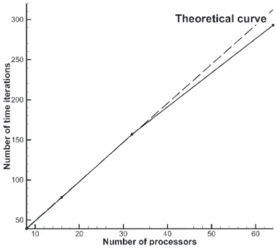
Thétis simulation tool has been parallelized for distributed memory architectures with MPI procedures. The parallelism is based on a grid decomposition to which the same simulation algorithm is applied on each processor. Each processor possesses its own data with specific node covering zones used to exchange the solutions at the boundaries of the processor data blocs. On each processor data block, a standard BiCGSTAB II solver is used which is preconditioned thanks to the local available unknowns through a Modified and Incomplete LU (MILU) method. The grid splitting is simply achieved by using a Cartesian cutting in each direction of the global mesh covering all the mesh blocks associated to each processor. More details on the parallelism is given in[76].

Specific developments have been investigated concerning the tracking of the particles over time in processor discrete space. Indeed, to build the phase function describing the local solid fraction and to update at each time step the physical characteristics of the one-fluid equations, the searching of particles interacting with a solid sphere belonging to a given processor must be undertaken. This type of algorithms has been often studied for many applications as the simulation of granular flows, the molecular dynamics or the universe gravitational forces. The algorithms change depending on the range of the interactions. For short range interactions the existing methods are able to find collisions between millions of particles. The most common algorithms use linked list approach[77,78], Verlet list [79] or a combination of the two

[80]. These algorithms are designed to deal with millions of particles efficiently. In our case they are not straightforwardly required because the number of considered particles is around several thousands and the number of CPU used for the

Fig. 7. Searching of particle collision inside a CPU box distribution of 10×10 in two dimensions – the red particle is detected to interact with green particles whereas no interaction is considered with the blue ones. (For interpretation of the references to color in this figure, the reader is referred to the web version of this article.)

simulations is determined by the needs of the fluid solver and the expected precision of the physical solution. However, brute force algorithm that search all the collisions between all the particles have a complexity of

O(

N2

p

)

if Np is the

number of particles. The time spent in searching collisions becomes important, i.e. comparable or larger than the solving time of the Navier–Stokes equations, for Np

>

500 with such a direct approach. A finer implementation using for example

octree structures will be required in the future to improve this aspect.

As a consequence, it has been decided to implement a cell-list approach to reduce the CPU time involved by the particle searching. The main idea is to split the physical space in boxes, and to search for collisions between particles only in a given box and the boxes around, as illustrated inFig. 7. Two conditions are necessary, the particles cannot pass through a box during a time step and the length of the boxes cannot be lower than the particle radius. The first condition is satisfied by assuming a CFL condition less than 1. The second condition have to be respected by the definition of the boxes. In our case, the CPU boxes generated by the Cartesian splitting of the global mesh are optimum for the solver with a number of cells of about 303. As the particle considered in our simulations have between 8 and 15 grids cells per radius, this condition is always fulfilled. Therefore, the use of the CPU boxes for the searching algorithm is a simple and efficient solution. In addition, this choice minimizes the communications between CPU.

2.8. Sum up of the implemented Eulerian–Lagrangian algorithm

The global algorithm used to solve one time iteration of fluid–particle interaction with the ITPM, the augmented La-grangian approach and the LaLa-grangian VOF particle tracking is summarized in Fig. 8. The first part of this work flow is devoted to predicting the position of the particle at time

(

n

+

1

)1

t through an extrapolation of their trajectories. The

four-way coupling forcing terms Fn_siare deduced from the particle interaction at this tentative position. The mass and momentum equations are then solved in both fluid and solid zones to obtain the pressure and velocities at time

(

n

+

1

)1

t. The particles

are finally advected in a Lagrangian way with the new velocity field. At the end of each time iteration, Lagrangian positions of the particles are projected on the Eulerian grid to build Cn+1and the local densities and viscosities are updated according to Cn+1_{before starting the next physical time iteration. This last procedure allows to penalize the solid behavior according}

to penalty viscosities in the cells belonging to the particles and also to account for buoyancy effects through the density variations.

3. Numerical and physical validations in dilute particle-laden flows

On a general point of view, the development of the ITPM method started in 1997 and is associated to previous works and publications. The complete and second order version of the method with collisions which is presented here is original. Specific validation test cases are reported here to demonstrate the numerical and physical capabilities of the method. How-ever, the reader is encouraged to refer also to previous publications[32]or[33]for complementary test cases such as the well-known Drafting–Kissing–Tumbling (DKT) problem.

3.1. Settling of a cylindrical shape particle

The settling of a cylindrical shape particle is first considered in two dimensions in order to characterize the effect of numerical parameters such as the solver, the augmented Lagrangian parameter or the magnitude of the viscous penalty

Fig. 8. Work-flow of the four-way coupling with the ITPM associated to augmented Lagrangian approach and Lagrangian VOF particle tracking.

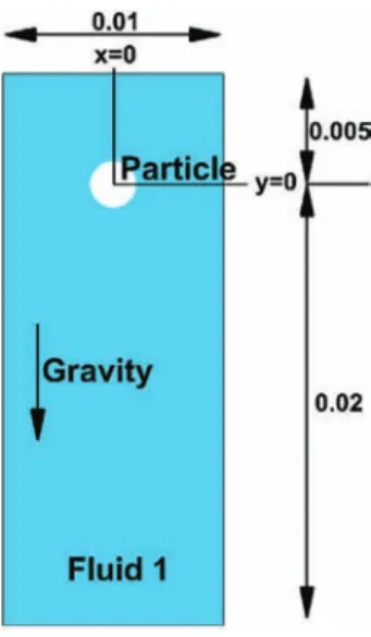
Fig. 9. Definition sketch of the settling of a cylindrical shape particle.

viscosity on the accuracy of the ITPM. The boundaries of the numerical domain are walls with a no-slip condition. A con-vergence study is also provided. The definition sketch of the problem is illustrated inFig. 9. At low Reynolds number, the analytical developments of Faxen[50]can be used to estimate the resistance force Fr of the fluid on the cylindrical shape

particle and its final settling velocity U∞. This reference velocity will be used to discriminate the most efficient numerical