a publisher's https://oatao.univ-toulouse.fr/27232
https://doi.org/10.1029/2020EA001118
Drilleau, Mélanie and Beucler, Éric and Lognonné, Philippe,... [et al.]MSS/1: Single͈Station and Single͈Event Marsquake Inversion. (2020) Earth and Space Science, 7 (12). 1-37. ISSN 2333-5084
Mélanie Drilleau1,2 , Éric Beucler3 , Philippe Lognonné1 , Mark P. Panning4 , Brigitte Knapmeyer‐Endrun5, W. Bruce Banerdt4, Caroline Beghein6,7 , Savas Ceylan8 , Martin van Driel8 , Rakshit Joshi9 , Taichi Kawamura1, Amir Khan8,10 ,
Sabrina Menina1 , Attilio Rivoldini11 , Henri Samuel1 , Simon Stähler8 , Haotian Xu6 , Mickaël Bonnin3, John Clinton8, Domenico Giardini8, Balthasar Kenda1 , Vedran Lekic12 , Antoine Mocquet3 , Naomi Murdoch2 , Martin Schimmel13 , Suzanne E. Smrekar4 , Éléonore Stutzmann1 , Benoit Tauzin14,15 , and Saikiran Tharimena4
1Institut de Physique du Globe de Paris, Sorbonne Paris Cité, CNRS F‐7500511, Université Paris Diderot, Paris, France, 2ISAE‐SUPAERO, Toulouse University, Toulouse, France,3Laboratoire de Planétologie et de Géodynamique, Université
de Nantes, Université d'Angers, Nantes, France,4Jet Propulsion Laboratory, California Institute of Technology, Pasadena, CA, USA,5Bensberg Observatory, University of Cologne, Cologne, Germany,6Department of Earth, Planetary, and Space
Sciences, University of California, Los Angeles, CA, USA,7Lunar and Planetary Institute, Houston, TX, USA,8Institute for Geophysics, ETH Zürich, Zürich, Switzerland,9Max Planck Institute for Solar System Research, Göttingen, Germany, 10Institute of Theoretical Physics, University of Zürich, Zürich, Switzerland,11Royal Observatory Belgium, Brussels,
Belgium,12Department of Geology, University of Maryland, College Park, MD, USA,13ICTJA‐CSIC, Barcelona, Spain, 14Laboratoire de Sciences de la Terre, Universit de Lyon I, CNRS and Ecole Normale Suprieure de Lyon, UMR5570,
Villeurbanne, France,15Research School of Earth Sciences, The Australian National University, Canberra, ACT, Australia
Abstract
SEIS, the seismometer of the InSight mission, which landed on Mars on 26 November 2018, is monitoring the seismic activity of the planet. The goal of the Mars Structure Service (MSS) is to provide, as a mission product, thefirst average 1‐D velocity model of Mars from the recorded InSight data. Prior to the mission, methodologies have been developed and tested to allow the location of the seismic events and estimation of the radial structure, using surface waves and body waves arrival times, and receiver functions. The paper describes these validation tests and compares the performance of the different algorithms to constrain the velocity model below the InSight station and estimate the 1‐D average model over the great circle path between source and receiver. These tests were performed in the frame of a blind test, during which synthetic data were inverted. In order to propagate the data uncertainties on the output model distribution, Bayesian inversion techniques are mainly used. The limitations and strengths of the methods are assessed. The results show the potential of the MSS approach to retrieve the structure of the crust and underlying mantle. However, at this time, large quakes with clear surface waves have not yet been recorded by SEIS, which makes the estimation of the 1‐D average seismic velocity model challenging. Additional locatable events, especially at large epicentral distances, and development of new techniques to fully investigate the data, will ultimately provide more constraints on the crust and mantle of Mars.1. Introduction
Because of its higher‐resolving power relative to other geophysical methods for sounding the interior of a planetary body, seismology has played a prominent role in the study of the interiors of Earth and Moon. This is one of the primary reasons for landing a seismometer on Mars with the InSight mission (Banerdt et al., 2013). The InSight (Interior Exploration using Seismic Investigations, Geodesy and Heat Transport) lander successfully delivered a geophysical instrument package to the Martian surface on 26 November 2018, including broadband and a short‐period seismometer instrument package called SEIS (Seismic Experiment for Interior Structure) (Lognonné et al., 2019). Although not buried but deployed at the Martian surface under a Wind and Thermal Shield, SEIS is specifically designed to record marsquakes and meteoritic impacts under Martian conditions, with a very low noise level (see Lognonné et al., 2020, for noise levels, as compared to the prelaunch estimation provided by Mimoun et al., 2017). Most of our knowledge about the internal structure of Mars has been inferred from geodesy data that has been supplemented with assumptions about the bulk composition of Mars. From the precise tracking of ©2020 The Authors.
This is an open access article under the terms of the Creative Commons Attribution License, which permits use, distribution and reproduction in any medium, provided the original work is properly cited.
Special Section:
InSight at Mars
Key Points:
• In the framework on the InSight mission, a synthetic seismogram using a 3‐D crust and a 1‐D velocity model below is proposed • This signal is used to present
inversion methods, relying on different parameterizations, to constrain the 1‐D structure of Mars • The results demonstrate the
feasibility of the strategy to retrieve VSin the crust, and a fairly good
estimation of the Moho depth
Correspondence to: M. Drilleau,
Citation:
Drilleau, M., Beucler, É., Lognonné, P., Panning, M. P., Knapmeyer‐Endrun, B., Banerdt, W. B., et al. (2020). MSS/1: Single‐station and single‐event marsquake inversion. Earth and Space Science. 7, e2020EA001118. https://doi. org/10.1029/2020EA001118
Received 30 JAN 2020 Accepted 17 JUN 2020
spacecraft orbiting Mars, the static gravityfield and dynamic gravity field have been determined, and the tracking of surface landers allows for the determination of the planet's precession rate. By combining the sta-tic gravityfield and the precession rate, the moment of inertia is determined from which the mass distribu-tion within the planet can be constrained. Supplementing the gravityfield data with topographic data allows constraining the structure of the crust, whereas the dynamic gravityfield or tides allow constraining the core radius and the rigidity of the mantle. Constraints about the bulk composition of the planet are deduced from a large set of Martian meteorites, in situ rock analysis obtained from Martian rovers, surface spectroscopy, and assumptions about how the planer formed. All these constraints have allowed for several estimates of the internal mechanical properties and compositional structure of Mars (e.g., Baratoux et al., 2014; Khan et al., 2018; Mocquet et al., 2011; Neumann et al., 2004; Plesa et al., 2015; Rivoldini et al., 2011; Smrekar et al., 2019; Sohl & Spohn, 1997; Verhoeven et al., 2005). However, these models suffer from the intrinsic nonuni-queness of any gravity data inversion, in particular with respect to the structure and thickness of the crust, structure, and composition of the mantle, including the existence and depth of discontinuities, and the core size.
The InSight mission extends planetary seismology to Mars. Seismic data will be integrated with geophysical measurements to determine details of the internal structure and evolution of another terrestrial body for the first time. However, the determination of the internal velocity structure and the location of the seismic sources using only one station is a challenge. Routine operations in the InSight team are split into two ser-vices: the Mars Structure Service (MSS) and the Marsquake Service (MQS), which are responsible for de fin-ing structure models (Pannfin-ing et al., 2017) and seismicity catalogs (Clinton et al., 2018), respectively. While the two tasks are intimately related and require constant feedback and interaction, these two services pro-vide a structure to ensure the mission will meet its science goals.
Following early works (Khan et al., 2016; Panning et al., 2015, 2017), the MSS team has developed several other different inversion algorithms in order to retrieve thefirst 1‐D‐averaged models of Mars from single station seismic data. To deal with the large inescapable uncertainties associated with the quake parameters and 1‐D structure model from a single station, we developed probabilistic inversion strategies with several types of seismic observables: body wave phase arrivals, surface waves, and receiver functions (RFs). In all cases, significant efforts have been devoted to the modeling approaches: when data are limited, they are indeed keys for understanding the significance of the resulting models.
The goal of this paper is to present the results of a blind test in terms of structure, in order to show how MSS can investigate Mars's interior using a variety of well‐suited methods performed on a single high‐quality seis-mogram. We took as“blind data” a synthetic seismic event and its associated broadband seismogram, com-puted within a 3‐D crust overlaying a 1‐D model from the Moho discontinuity to the core. All parameters used in the forward modeling were unknown to those in charge of inversions. This single synthetic data set was then used to perform inversions for inferring both Marsquake parameters (location, depth, origin time, and moment tensor) and interior velocity models.
This study provides a clear framework to describe the methods employed by the MSS demonstrated on a data set for which results can be compared to the ground truth. Clearly, this remains a“best case” scenario for the resolving power of a single event, but it is an important demonstration of the planned approaches. The dif-ferent algorithms handle surface waves and/or body waves, RFs, and consider difdif-ferent parameterizations. Wefirst describe the synthetic input data, the traveltime measurements, and then detail the different inver-sion techniques for investigating the deep structure of Mars, and quake location. Constraints from RFs, which provide information on crustal structure directly below the receiver, and from surface waves and body waves, which average the structure over the great circle path between source and receiver, are considered independently here. Wefirst present, discuss, and compare the results of six different methods estimating the 1‐D average model over the great circle path between source and receiver. Second, we described the results from a local study below the station, by inverting RFs. The results clearly highlight the nonunique-ness of the solution and enhance the approach considered by the MSS of using several complementary meth-ods to fully investigate the data. We also demonstrate the feasibility to estimate the attenuation of Mars, using a single event.
Up to now and despite very low noise (Lognonné et al., 2020), most seismic event waveforms recorded by SEIS do not exhibit clear phase arrivals, and none have observable surface waves (Giardini et al., 2020;
Lognonné et al., 2020). Only two marsquakes show clear P and S arrivals with picking errors smaller than 2 s for P and S, which means that several methods developed in the framework of the MSS cannot yet be used with SEIS data. The core of the proposed methods will, therefore, be applicable if Martian seismicity provides soon larger quakes with body wave phases and first orbit surface wave dispersion, or one event large enough to record multiple orbit surface waves. A section is therefore dedicated to the inversion results using only body wave arrival times. The results show a strong trade‐off between the seismic velocity profile and the quake loca-tion, which prevents a clear estimation of the crust and mantle velocity structure, as well as the crustal thickness. In the absence of surface waves, the work of the MSS becomes even more challenging, and new methods need to be developed in order to fully take advantage of all the informa-tion contained in the SEIS data.
2. Synthetic Waveforms
Two blind tests were performed prior to landing to validate the SEIS data processing. Thefirst one was for the detection and characterization of events and was linked to the MQS activities (Clinton et al., 2018). We refer to Clinton et al. (2017) and van Driel et al. (2019) for further details on the MQS tests results. The MSS blind test was on its side designed for practicing and improving the procedures and methods aim-ing to invert Mars's internal structure from SEIS data.
To mimic expected Mars conditions before InSight touchdown, the synthetic test data set included four Earth day long seismic recordings (three‐component VBB data at 2 and 20 sps, single‐component combined VBB vertical channel at 10 sps) as well as auxiliary channels such as pressure, magnetometer, wind speed, wind direction, and atmospheric temperature.
A single marsquake is hidden in the continuous signal, which is contaminated by Martian noise based on prelaunch hypotheses (Mimoun et al., 2017). The event's parameters are detailed in Table 1. The background structural model, or 1‐D base model, for quake simulations was chosen from a suite of 14 models (Clinton et al., 2017). In order to make this blind test challenging, an anomalous 1‐D model is considered, with a tem-perature profile in the crust and mantle close to the liquidus (Khan et al., 2018). Such a temtem-perature profile gives a seismic velocity profile located in the extreme lower bound of the expected velocity models of Mars (Smrekar et al., 2019). The source parameters were randomly chosen.
In the MQS exercise focused on event detection and location (Clinton et al., 2017; van Driel et al., 2019), the seismograms were computed in a 1‐D model, which greatly simplified the analysis. The goal here is to include unexpected behavior as well as 3‐D effects on surface waves due to crustal heterogeneities (Bozdagˇ et al., 2017). To this end we performed a full 3‐D computation (Afanasiev et al., 2019) for S waves and surface waves to the shortest period of 5 s and merged the trace in the time domain just before the S wave arrival with 1‐D synthetics (Bozdagˇ et al., 2017; Nissen‐Meyer et al., 2014; van Driel et al., 2015) accurate to 1.5 Hz. This is moti-vated by the observation that the attenuation of the model would not allow shorter period teleseismic S waves above the noise level in any case. For consistency, the 1‐D synthetics are aligned to the 3‐D P wave arrival time by cross correlation of the 1‐D and 3‐D synthetics in the frequency range where both are well resolved. The seismic noise model comes from the SEIS noise model (Mimoun et al., 2017). This comprehensive model includes prelanding estimates of the key contributors to the seismic noise: the pressure noise (Kenda et al., 2017; Murdoch et al., 2017a), the wind‐generated mechanical noise (Murdoch et al., 2017b), the thermal and magnetic noise (Mimoun et al., 2017), and the instrument self‐noise (Lognonné et al., 2019). Further details about how this noise was integrated into the synthetic waveforms are provided in Clinton et al. (2017).
3. Traveltime Measurements
3.1. MQS EstimatesSince raw synthetic waveforms are supposed to mimic the worst‐case scenario planned for data transmission of the continuous signal acquired on Mars, they are provided at a sampling rate of 2 Hz.
Table 1
Parameters of the MSS Blind Test Event for Computed and True Locations
Event parameters Computed origin True origin
Origin time (UTC) 2019‐01‐03 15:00:53 2019‐01‐03 15:00:30
Latitude 26°S 26.443°S
Longitude 53°E 50.920°E
Depth 36 km 38.4 km
Magnitude MsM¼ 3.7 (Mw ¼ 4.2) Mw¼ 4.46
Distance 85.7° 87.6°
Back azimuth 243.0° 243.4°
Note. MsM is the magnitude derived for Mars using the surface wave amplitudes (Böse et al., 2017).
The probabilistic location algorithms that MQS utilizes are explained in Panning et al. (2015) and Böse et al. (2017) in detail. MQS uses a collection of approximately 2,500 Mars models, which is a combined set of inputs from all members of the InSight science team. The MQS algorithms operate on a traveltime database for the most common body wave phases at all distance ranges, as well as surface wave arrivals in predeter-mined frequency bands. Traveltimes are computed using the TauP package of Crotwell et al. (1999). Table 1 summarizes the computed location and the input parameters. Although direct and major arc surface wave arrivals were visible, it was not possible to identify a clear arrival of multiorbit surface waves (R3). Further, 3‐D traveltime corrections for surface waves were not implemented at the time of the test. Therefore, the MSS location was computed solely using body wave phases. The event depth (∼36 km) was constrained using a clear pP arrival 14.4 s after the P wave. The event magnitude (MsM¼ 3.7) is computed using the direct Rayleigh wave arrival. Following Böse et al. (2017), this value scales to approximately Mw¼ 4.2–4.3.
3.2. Body Waves
Onset times are picked by various contributors, they are gathered by the institution names (IPGP, ISAE, ETH, MQS, and LPG), and the major seismic phases are represented in Figure 1. Concerning the compres-sional seismic phases (i.e., P, pP, and PP), there is a very good agreement between all manually performed picks, whereas we observe a slightly larger discrepancy for shear wave onset times.
The mean value for the arrival time of the direct P wave is 2019‐01‐03T15:09:54.5 (UTC) with a standard deviation lower than 0.1 s; the corresponding value for the arrival time of the direct S wave is 2019‐01‐03T15:18:31.1 (UTC) with a standard deviation of 3.6 s. The larger uncertainty for the direct S phase is mostly due to a low‐amplitude, emergent direct shear wave arrival, which is moreover almost concomitant with a high‐frequency signal, which has not been identified, and no clear S wave coda (Figure 2).
To determine back azimuth (in the horizontal plane) and arrival (in the vertical plane) angles of the direct P wave ray, we use an approach based on the analysis of the polarization of the incoming P wave energy. The seismogram is band‐pass filtered between 0.2 and 0.5 Hz in order to enhance long‐period particle motion around the hand‐picked P wave onset time. The window of interest starts 1 s before the picked P wave arrival and ends 5 s after.
The analysis is based on the approach from Jurkevics (1988); that is, we solve an eigenvalue problem on the 3‐D particle motion to find the eigenvector that is a good approximation of the P wave vector. Its orientation and polarity are then used to recover the back azimuth of the P wave (Figure 3a). To strengthen the analysis, which is very sensitive to noise, we also perform a Monte Carlo exploration of the 3‐D particle motion obtained from the 6 s analysis window. Two hundred sets of samples from between 60% and 90% of all the particle motion samples are randomly selected, and they are used to compute the average back azimuth. This process is repeated 200 times so that the preferred back azimuth value (Figure 3b) is given by the mean and the standard deviation of the distribution (given by a kernel density estimation). The inferred value for the back azimuth is in agreement with the source location.
The arrival angle is computed following the same strategy (Figure 4). The back azimuth angle is used to rotate the seismogram in order to use a vertical/radial/transverse reference frame. We also limit the analysis to the radial/vertical particle motion as almost all of the P wave energy should be confined to this plane. 3.3. Surface Waves
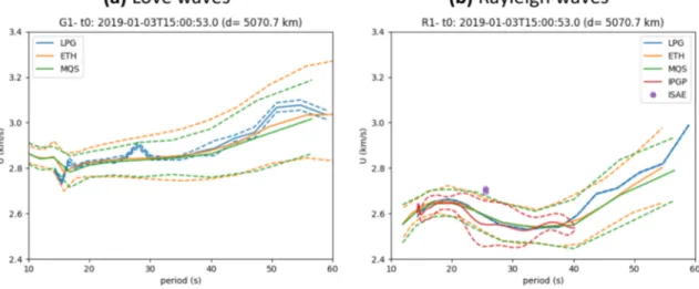
Both Love waves on the transverse component and Rayleigh waves on the two other components (Figure 2) are easily recognizable in the seismograms. Most of the surface wave energy is between 10‐ and 60‐s period. The rotation in the great circle plane, defined by the source and the receiver, efficiently isolates Love waves that travel faster than Rayleigh waves. Two types of observables can be derived from raw data: discrete group velocity values at different frequencies and dispersion analyses using probability density functions (pdfs) of the energy.
As for body waves, arrival times for Love and Rayleigh waves are manually picked and are converted into group velocities for the different wave trains. Figures 5a and 5b exhibit the group velocity curves, with the corresponding uncertainties, between 10‐ and 60‐s period, obtained from the G1 and L1 wave trains (travel path along the minor arc between the source and the receiver). They are computed using the origin time and
the quake location as given by the MQS (Table 1). The major arc wave trains (i.e., G2 and R2) are picked with good consistency between the various contributions, but since they are not used for inversions, they are not shown here. Only two contributors picked G3 and R3 arrival times in a very narrow frequency band (between 25‐ and 30‐s period).
For both Love and Rayleigh waves, all contributions are very consistent over the whole frequency range. Almost all group velocity values are within the uncertainties defined by the ETH and the MQS. This feature is consistent with a mean model for which body wave velocities are increasing as a function of depth. 3.4. Dispersion Analysis
In addition to the arrival time picks for the different wave trains of surface waves, we present a dispersion analysis of thefirst fundamental mode waveforms (Figures 6a and 6b). Both Love and Rayleigh waves are
Figure 1. (a–d) Body wave picks are represented by red vertical lines. For each seismic phase, the corresponding time window is 150 s long and is centered around thefirst picked value (top trace). When it has been quantified during the picking step, the uncertainties are showed in pink. The band‐pass filter characteristics and the component are indicated above each plot.
Figure 2. Synthetic traces after rotation in the source‐to‐receiver great circle plane and filtered between 2‐ and 100‐s period. Direct P waves arrival is highlighted in pink, S waves in violet, and surface waves (both Love and Rayleigh) are present in the green window.
Figure 3. Illustration of the back azimuth computation from the polarization analysis of the ZNE particle motion. (a) Particle motion in the EN plane (solid black line) with the recovered back azimuth (red dashed line). (b) Kernel density estimation (Gaussian kernel with 1° bandwidth) of the back azimuth distribution (solid black line) with the mean of the distribution (dashed red line). The retrieved back azimuth value is 242° ± 1°.
filtered using 20 narrow Gaussian band‐pass filters, and each trace is converted into energy using the envelope of the signal. The signal is then interpolated on a regularly discretized group velocity axis, assuming an origin time value and an epicentral distance (the location from MQS is used, Table 1), and the whole window isfinally converted into probabilities, which is a slightly different version of the one described in Panning et al. (2015). The collection of pdfs of group velocities displayed in Figure 6, therefore, can be seen as a dispersion diagram. Two histograms, corresponding to two different frequencies, are displayed above the dispersion diagrams to illustrate this approach.
When looking at the dispersion for periods greater than 12 s, it is clear that group velocities are unimodal, and the maximum of each pdf matches almost perfectly the picked values shown in Figure 5. At shorter per-iods, we observe a sharp discontinuity in both pdfs. They are highlighted by bimodal distributions (see red histograms in Figures 6a and 6b). This feature affects both Love and Rayleigh waves and prevents inversions for periods shorter than 10–12 s. We do not observe any robust correlation between Love and Rayleigh sig-nals that could indicate the presence of anisotropy (Babuska & Cara, 1991), and we interpret this short‐period energy in terms of 3‐D propagation effects. Since we do observe a 2π phase shift between
Figure 4. Illustration of the incidence computation from the polarization analysis of the ZR particle motion. (a) Same as Figure 3 but for ZR particle motion (black solid line) and incidence angle (red dashed line). (b) Same as Figure 3 for incidence angle. Incidence angle¼ 22° ± 1°.
Figure 5. (a and b) Surface wave group velocities computed from manually picked arrival times. The value for origin time and epicentral distance are given at the top; they correspond to the MQS solution.
longitudinal and vertical components (see Figure 7 for the fundamental mode), we are facing retrograde par-ticle motion. This spurious signal can, therefore, be associated with multipathing since there is a large crus-tal thickness anomaly (up to 20–25 km) in the source neighborhood. Hence, this energy can propagate along the same travel path and therefore reach the receiver with no significant arrival angle anomaly (Woodhouse & Wong, 1986).
3.5. Particle Motion
As explained in Panning et al. (2015), the particle motion of the Rayleigh wave fundamental mode can be used for back azimuth determination but it can be used as well to investigate the physical properties of the crust. In a velocity model showing a substantive velocity increase as a function of depth, Rayleigh waves are characterized by a retrograde elliptical particle motion. In many cases on Earth, the particle motion of the Rayleigh wave fundamental mode is retrograde while higher modes propagate in prograde motion. Very few studies report prograde observations of the fundamental mode (Tanimoto & Rivera, 2005), and this effect due to propagation through a thick sedimentary basin. In the case of a retrograde motion, once the horizontal components are rotated into the source‐receiver great circle reference frame, the longitudinal (in the direction of positive minor arc propagation) isπ/2 phase‐shifted with respect to the vertical. It means that horizontal displacements are in phase with the Hilbert transform of the vertical component multiplied by−1 (Gribler & Mikesell, 2019). Thus, such a comparison between longitudinal and vertical waveforms can bring some information on the near‐surface properties.
The result of the particle motion analysis is displayed in Figure 7. For 170 time samples (blue and red points), which corresponds approximately to the duration of the Rayleigh fundamental mode wave train, the nor-malized cross correlations between the longitudinal component and the Hilbert transform of the vertical multiplied by−1 (associated with blue color) and +1 (in red) are computed. Each color point represents the zero‐lag value of these cross correlations. In order not to be affected by the length of the time window used for the computations, all possible lengths between 150 and 350 s are tested and the best zero‐lag value is retained.
It is obvious that (i) all blue points are positives which is consistent with a retrograde particle motion and (ii) the largest value is almost equal to one and it corresponds to the beginning of the Rayleigh wave train (thick blue line). The top graph on the left (Figure 7) shows for this time window that the normalized cross
Figure 6. Dispersion analysis of thefirst wave trains of surface waves. The waveforms corresponding to (a) Love and (b) Rayleigh are band‐pass filtered in 20 narrow band Gaussianfilters between 8‐ and 50‐s period. For each frequency, the envelope of the filtered signal is converted into a probability density function of group velocities and are plotted in gray scales. Two histograms (red for short periods and green for long periods, as indicated by the colored lines in the dispersion diagrams) are shown above the dispersion diagrams. For Love waves and vertical Rayleigh waves, the red histograms are shown for period values of 10.7 and 12.9 s, respectively. The green histograms corresponds to a period of 30.8 s.
correlation between the longitudinal and−HðZÞ (blue signal) is almost identical to the autocorrelation of the longitudinal component (black signal). On the other hand, the best value for the cross correlation between longitudinal and positive Hilbert transform is for the last point (top graph on the right), which means that the corresponding time window is after the end of the Rayleigh fundamental mode wave train.
4. Estimation of the 1‐D Average Model Over the Great Circle Path Between
Source and Receiver
4.1. Methods
Six independent inversion algorithms were developed in order to retrieve the 1‐D average model along the minor arc. The goal here is not to produce a single model, but rather a family of models thatfit the data and are consistent with the most recent set of prior constraints. The main characteristics of each method are described in Table 2. This study spans a relatively wide range in terms of model parameterization from the standard seismic parameterizations over fully self‐consistent thermodynamic methods. Indeed, two main approaches are considered. One set of models (called M1) are parameterized in seismic velocity as a function of depth. A second set (called M2) is obtained with models parameterized by geodynamical para-meters like temperature and composition. Assuming thermodynamic equilibrium, the seismic velocity pro-files can then be calculated using first thermodynamics principles with experimentally derived parameters for candidate minerals. The strength of the M1 models is that they are able to mimic“exotic” models if the composition and/or temperature are variable along the wave path, or if the equilibrium assemblage is not reached. Their weakness is that they do not take into account constraints from mineral physics, nor geo-physical data (e.g., moment of inertia, tidal response, and thermal evolution of the planet). The M2 method permits the application of tight constraints on velocity structure with a relatively limited data set, by produ-cing stable velocity models through the whole planet, in contrast to the M1 models which give some con-straints only at the depths where the data are sensitive. The M2 modeling approach is extremely powerful if we have very good prior constraints. However, the M2 models will not be representative of Mars if the prior assumptions on mineral physics turn out to be false or if the equilibrium assemblage is not reached. The
Figure 7. Bottom graph: Analysis of the particle motion of thefirst vertical Rayleigh wave train (black signal). Each color point (blue and red) represents the zero‐lag value of the normalized cross correlation between the longitudinal and the negative in blue (positive in red) Hilbert transform of the vertical component. Top graphs: For two time windows, the autocorrelation of the longitudinal component in black and the normalized cross correlation between longitudinal component and the Hilbert transformed vertical multiplied by−1 in blue and +1 in red. The top left graph shows that at 5,530 s the waveform on BHL component is perfectly matching−HðBHZÞ.
advantage of using these two complementary approaches is that comparisons between these two families could indicate regions of the models that are not well constrained by the data, or inconsistent with the physical assumption of the M2 modeling approach.
The inverse problem consists in retrieving the seismic velocity profiles as a function of depth from body waves and surface waves traveltimes measurements. The problem is, however, underdetermined, in the sense that several combinations of velocity profiles and locations can give similar arrival times. Due to the underdetermined nature of the problem, we mainly use Bayesian inversion techniques to obtain robust pdfs of seismic velocity profiles. This technique allows the investigation of a large range of possible models and provides a quantitative measure of the models' uncertainty and nonuniqueness. As such, it is well suited to our problem given the still poorly known nature of the Martian interior, as well as the low amount of iden-tified phase arrivals recorded by SEIS at this time (Giardini et al., 2020; Lognonné et al., 2020). The forward problems are computed with 1‐D structure, which allows the computations of several million forward pro-blems. The pdf of the a priori distribution, for each of the six methods, is displayed in Figure 8. In the follow-ing, the six methods are described in details. The M1 methods were initially developed for Earth applications and recently modified for Mars in preparation for the InSight mission. The M1a and M1b methods were modified from the previous work of Drilleau et al. (2013) and Panning et al. (2015, 2017). The M1c method is derived from Xu and Beghein (2019). The M2a method was already published in Khan et al. (2016, 2018), whereas the M2b and M2c methods were recently developed in the framework of the MSS.
4.1.1. M1 Models
M1a. The inversion algorithm is mainly based on the work of Drilleau et al. (2013) and Panning et al. (2015, 2017). The 1‐D VSmodels are parameterized with three layers in the crust, and with six Bézier points in the
mantle, which are interpolated using polynomial C1Bézier curves. The inverted parameters are the depth of the three layers in the crust and their VSvalues, the depth and VSvalues of the Bézier points in the mantle,
and the VP/VSratios in the three layers of the crust and the mantle. In total, 21 parameters are inverted to
describe the velocity model. The a priori conditions on the depths of the crustal layers are that the depth of thefirst and third layers cannot exceed 10 and 100 km, respectively. The Bézier points are randomly located between the Moho depth and the top of the core. The VSprofiles are randomly sampled within
rela-tively wide prior bounds, as shown in Figure 8a. In order to ensure a velocity jump at the Moho, we impose that VSof thefirst Bézier point in the mantle must be higher than VSin the third layer of the crust. The VP/VS
ratios are allowed to vary between 1.5 and 2.2. Simultaneously, a relocation of the quake is performed by moving the epicentral distance and the depth of the quake. For the blind test exercise, we choose to set the prior bounds relying on the uncertainties found by the MQS, between 80° and 95° and 25–45 km for the epicentral distance and the depth of the quake, respectively.
Table 2
Details of the Six Different Inversion Methods Used by the MSS
M1a M1b M1c M2a M2b M2c
Possibility of using yes no no yes yes yes
body waves only
Data surface waves surface waves surface waves surface waves surface waves surface waves
body waves body waves body waves body waves
(Figures 1 and 5, (Figure 6) (see section 4.1.1, (Figures 1 and 5, (Figures 1 and 5, (Figures 1 and 5,
MQS values) M1c) MQS values) MQS values) MQS values)
Relocation yes no yes yes yes yes
Inverse problem McMC McMC McMC McMC McMC grid search
Misfit function differential group waveforms traveltimes differential traveltimes
calculated on arrival times velocities and and arrival times
group velocities group velocities
Inverted VP, VS VP, VS, VS crust: VP, VS crust: VP, VS VP, VS
structure radial anisotropy mantle: composition mantle and core of a priori models
parameters and temperature convective temperature based on geodynamical
viscosity, parameters
activation energy, activation volume
To solve the inverse problem, we employ a Markov chain Monte Carlo (McMC) approach (e.g., Mosegaard & Tarantola, 1995). For each sampled model, we rely on the ray tracing algorithm of Shearer (2019) to compute body wave traveltimes. The surface wave velocity dispersion curves are calculated using the MINEOS pack-age (Masters et al., 2011) and are then converted to traveltimes using the randomly sampled epicentral dis-tance value. Since the origin time t0is typically unknown, we use differential times relative to the P wave
phase arrival. The cost function is then defined as follows:
C¼jðt
obs
S − tobsP Þ−ðtcalcS − tcalcP Þj
σSþ σP þ
jðtobs
pP − tobsP Þ−ðtcalcpP − tcalcP Þj
σpPþ σP
þ∑
N
jðtobs
R − tobsP Þ−ðtcalcR − tcalcP Þj
σRþ σP ;
(1)
where C computes the misfit between the observed and computed differential arrival times tS− tP, tpP− tP
and the sum of the misfit between the observed and computed differential arrival times tS− tRat each
fre-quency, taking into account the error barsσP,σS, σpP, andσRon P, S, pP, and Rayleigh waves arrival
times, respectively. Superscripts throughout refer to observations (obs) and computed data (calc). Inversion output consists of an ensemble of internal structure models thatfit the cost function.
Figure 8. A priori probability density functions of VSas a function of depth for M1 (a–c) and M2 (d–f) methods, considering that all the sampled models which are
in good agreement with a priori information are accepted. Blue and red colors are low and high probability, respectively. The black lines in (a) and (b) show the upper and lower prior bounds. At every kilometer in depth, the pdf values are computed by counting the number of profiles in each VSinterval of 0.05 km/s. For a given depth, the sum of the pdf over all the parameter intervals is equal to 100%.
M1b. In contrast with the previously described method for M1a models, M1b models are inferred using infor-mation carried by surface waves only, considering afixed location of the marsquake (see Table 1, computed origin). The anisotropy is taken into account in a joint Love/Rayleigh inversion scheme. The data space is composed here by two distinct ensembles of a priori pdfs of both Love and Rayleigh group velocities (Figures 6a and 6b; see section 3 for details). The parameter space in our case is composed by four subspaces (compressional and shear velocities, density, andξ) as a function of depth. The inverse procedure relies on McMC explorations of the whole parameter space in order to compute a posteriori probability densities for each subspace. It is an improved version of the concepts presented in Panning et al. (2015, 2017) in the sense that the forward problem can now take into account for anisotropy.
Under the hypothesis of a transversely isotropic medium (Love, 1892), the joint inversion of the two types of surface waves allows constraining
ξ ¼V2SH
V2 SV
; (2)
where VSHand VSVare the horizontally and vertically polarized shear wave velocities, respectively.
For each 1‐D trial model defined by ρ(z), VP(z), and VSV(z) and VSH(z), a modal summation theory (Masters
et al., 2011) is used to compute the corresponding Love and Rayleigh group velocities. Each group velocity curve can be compared directly to the dispersion diagrams (Figure 6), which quantifies the relevance of the trial model in the data space. This means that, in contrast to widely used misfit computations within Bayesian explorations and relying on gaussian assumptions, the goodness of fit is measured by the likelihood,
Lða1;…; amÞ ¼ ∏ N
i¼1Pðνi; a1;…; amÞ: (3)
The likelihood function is then the product of the individual probabilities sampled by the group velocity curves (which represent the state of a given parameter configuration a1,… , amevaluated at each frequencyνi).
To compute a large ensemble of model shapes, 70 Markov chains are running in parallel, and each chain uses a given geometrical constraint for the generated models between 0‐ and 140‐km depth. As introduced by Drilleau et al. (2013), each model shape is controlled by piecewise C1 Bézier curves (Bézier, 1977; Farin, 1993), based on several anchor points. Two anchor points at 0‐ and 140‐km depth bound the tion range and all intermediate points are shared by two following Bézier curves. To ensure a broad explora-tion of the model space, each Markov chain is associated with a unique random seed and an amount of Bézier points, which vary between 5 and 9. This amount varies between all chains but does not vary within a single chain during iterations. The minimum authorized distance between each anchor point is set to 8 km, which allows to generate models varying smoothly over the whole depth space as well as sharp discontinuities.
After afirst stage of large wavelength exploration (cold runs), the posterior probabilities are constructed with the 6,000 models showing the lowest misfit values inferred during the 70 × 5,000 iterations (once they have been downsampled in order to prevent covariances).
M1c. The technique used here is a waveform modeling method based on a hierarchical transdimensional Bayesian approach to measure the dispersion of fundamental and higher mode surface waves. It was initially developed by Xu and Beghein (2019) for Earth applications and recently modified for Mars in preparation for the InSight mission. A McMC technique is used to seek a distribution of 1‐D shear wave velocity models that represent the phase velocities of the fundamental and/or higher mode surface waves recorded between a seismic source and a receiver on a single seismogram. The distribution of 1‐D models is then used to calcu-late dispersion curves and uncertainties, and tests are performed to assess the reliability of the measure-ments. Fundamental mode surface waves are generally much easier to isolate on the seismogram than the overtones, and thus, their dispersion is often more reliably measured.
An advantage of using a hierarchical transdimensional Bayesian approach lies in the fact the depth parame-terization does not have to befixed a priori since the algorithm lets the data control the complexity of the
solution while being parsimonious. Another great advantage is that it can alsofit the data noise, which reduces the risk of mapping unknown noise into the velocity model and associated phase velocities. In addi-tion, the source parameters can be included among the unknowns, thereby allowing source estimate uncer-tainties to be propagated into the model unceruncer-tainties. Since we are working with only one seismometer on Mars, uncertainties in the source may be larger than we are used to on Earth and it is well known that wave-form inversions can be affected by trade‐offs between source and structure. Here, we present results based on the source parameters obtained by the MQS (Table 1).
A notable difference between performing phase velocity measurements with waveform modeling on Mars compared to Earth is that we do not yet have a reliable reference model for Mars. For Earth applications, a reference dispersion curve calculated for a reference interior model is often used to prevent cycle skipping, which can affect the measured phase velocities. In the absence of a reliable reference model for Mars, we included the envelope of the waveform in the cost function instead, as was done previously by Yoshizawa and Ekström (2019).
The vertical component of the blind test data werefiltered in different frequency bands, but no clear higher mode Rayleigh waves were visible. Fundamental mode Rayleigh waves, however, were clearly seen at per-iods between 25 and 50 s. The method employed here is not fully nonlinear due to the high computational cost of the forward problem. First, a synthetic reference seismogram and corresponding eigenfunctions are calculated using the fully nonlinear normal mode summation code MINEOS (Masters et al., 2011) and a starting model. The synthetic seismogram is then updated at each iteration using a linear approximation. Tofind a reference model, we first tested several published 1‐D Mars interior models (Sohl & Spohn, 1997; Zheng et al., 2015) and found that one of the Zheng et al. (2015) models predicted a synthetic seismogram that resembles thefiltered blind data in the same period range the best, apart from a time shift of about 2 s. We then performed a rough grid search to modify the VSprofile in order to bring the synthetic waveform
and the blind test waveform closer together in time. The misfit was calculated with a L2norm. We used the
resulting VSmodel as our reference model.
The VSprofile is described by a variable number k of interpolation points, the vertical and horizontal
posi-tions of which define the depths at which VSis perturbed and the amount by which VSis perturbed relative
to a reference model, respectively. The prior for VSis a uniform distribution of ±10% around the reference
model (Figure 8c), and the Moho is allowed to vary by ±5 km around the reference value and two different reference values are tested to account for the prior uncertainty on crustal thickness. Perturbations in P wave velocity are assumed to be proportional to those in VS, as often done for Earth applications (e.g., Yoshizawa
& Ekström, 2019). We compared results for which density anomalies were neglected and scaled to dVS
(dρ/ρ ¼ 0.3dVS/VS) and found no significant change in the resulting VSmodels.
We compared VSprofiles obtained with reference models with different Moho depths, namely, 50‐ and 75‐km
depth. Note that by changing the crustal thickness in the reference model, we also had to adjust the reference VSin order to time shift the synthetic waveform and bring it closer to the observed blind surface waveform.
We used a uniform prior for source parameters with a range of allowed values based on the uncertainties esti-mated by the MQS. Only the source latitude and longitude were kept constant. On average, the misfit for models with a 50‐km‐thick crust is smaller than that of models with a 75‐km‐thick crust. However, after per-forming F tests (Menke, 2012) on several of the best models in each case, we found that the misfit difference is not significant due to the difference in the number of model parameters. The waveform and envelope inver-sion is therefore unable to distinguish between models with a 50‐ or 75‐km‐thick crust. In the discusinver-sion in section 4.2, only the results using the 50‐km‐thick crust reference model are shown.
Because the envelopefit can be strongly affected by the noise level, we also tested whether the inclusion of group velocity data instead of the envelope affects the results. To do this, we modified the cost function to include group velocity measurements. Wefind that the velocity profiles do not strongly differ from those using the envelope measurements only, but the range of allowable VSmodels is slightly larger with group
velocities than with the envelope. 4.1.2. M2 Models
M2a. In the following, we describe a method for inverting P and S wave body wave traveltimes and surface wave dispersion data jointly as outlined in Khan et al. (2016). To compute radial profiles of density, P and S
wave velocity, and shear attenuation, we rely on an average bulk Martian mantle composition and model areotherm using thermodynamic principles, mineral physics data, and viscoelastic modeling as described in Khan et al. (2018). Our Martian model is spherically symmetric and consists of three layers: a silicate crust and mantle and a metallic core. Seismic properties in the three layers are determined in the following manner.
1. Mantle. We use the free‐energy minimization strategy of Connolly (2009) to determine stable mineralogy, elastic moduli, and density along self‐consistently computed mantle adiabats for a given bulk composi-tion. The thermodynamic formulation of Stixrude and Lithgow‐Bertelloni (2005) including parameters as in Stixrude and Lithgow‐Bertelloni (2011) are employed for this purpose. Bulk moduli are estimated by Voigt‐Reuss‐Hill averaging, while the pressure profile is obtained by integrating the load from the sur-face boundary condition p¼ 105Pa. Mantle compositions are explored within the Na2O‐CaO‐FeO‐MgO‐
Al2O3− SiO2(NCFMAS) chemical model system, which accounts for more than 98% of the mass of the
mantle of the experimental Martian model of Bertka and Fei (1997).Estimates for the Martian mantle composition derive from geochemical studies of a set of basaltic achondrite meteorites, which are believed to originate from Mars (e.g., Dreibus & Wanke, 1985; Lodders & Fegley, 1997; McSween Jr, 1994; Mohapatra & Murty, 2003; Sanloup et al., 1999; Taylor, 2013; Treiman, 1986). Based on these analyses, the Martian mantle is found to contain∼17 wt% FeO, implying a Martian mantle Mg# of 75 (100 times molar Mg/Mg+Fe).
2. Crust. The crust is subdivided into three layers that are parameterized in terms of P and S wave velocity, and density, in addition to Moho thickness. To emulate the effect of porosity, we computed the aforemen-tioned physical properties by multiplying the thermodynamically computed seismic wave speeds and density in crustal layer i by a variable parameterϕ. The ϕiis determined fromϕi¼ ϕ0+ (1− ϕ0)(i/N) with
ϕ0being variable surface porosity and N the total number of crustal layers. This parameterization ensures
that crustal properties increase from the surface down to the Moho where porosity is expected to vanish due to pressure.
3. Core. Sulfur is believed to be the dominant light element in the core of Mars because other elements (e.g., silicon, oxygen, and carbon) do not have sufficient solubility in iron‐rich liquid at the relatively low pressures that are expected to have been maintained during core formation (e.g., Stevenson, 2001). Evidence in support of this comes from the observed depletion of chalcophile elements in the Martian meteorites, notably sulfur and the large value of the degree‐2 gravitational potential Love number. To compute depth‐dependent thermoelastic properties for the core, we use equations of state for liquid iron and liquid iron‐sulfur alloys, relying on the parameterization of Rivoldini et al. (2011) for a well‐mixed and convecting core.
4. Attenuation. The dissipation model adopted here is based on laboratory‐derived torsional forced oscilla-tion data on melt‐free polycrystalline olivine and is described in detail in Jackson and Faul (2010). The extended Burgers model of Jackson and Faul (2010) is preferred over other rheological models because of its ability to describe the transition from (anharmonic) elasticity to grain size‐sensitive viscoelastic behavior as a means of explaining the observed dissipation in the experiments on olivine.For present pur-poses, computations were conducted employing a single shear wave attenuation (Q) model at seismic frequencies (1 s) and a grain size of 1 mm. For the Martian crust and lithosphere, wefixed shear wave Qto 600 after PREM (Dziewonski & Anderson, 1981). As the core is assumed liquid, no shear attenuation is needed in the core. Dissipation in bulk is neglected and we assume Qκ¼ 104in line with terrestrial
applications (e.g., Durek & Ekström, 1996). Anelastic P and S wave speeds as a function of pressure, temperature, composition, and frequency are estimated from the expressions for the viscoelastically computed temperature‐, pressure‐, and frequency‐dependent moduli (further details may be found in Khan et al., 2018).
M2b. In this approach, we use a McMC joint inversion of body waves and surface wave seismic data, where the modeling of Mars's thermochemical history is part of the forward problem. In order to make reliable pre-dictions about the seismic data from interior structure models the present‐day thermal state of Mars is of fun-damental importance. To obtain a plausible present‐day thermal state of Mars, we simulate for each interior model its long‐term thermal evolution. The thermal evolution is calculated with a parameterized thermo-chemical model that depends on a small set of parameters and an initial temperature profile. Such approach, allows the long‐term planetary evolution to be accurately modeled at a reasonable computational cost.
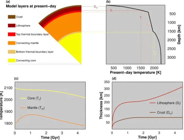
Our forward problem consists in sampling the model space by computing different thermochemical evolu-tions of a Mars‐like planet divided into several concentric and spherically symmetric envelopes (Figure 9a): a convecting iron‐sulfur liquid core (Rivoldini et al., 2011), surrounded by a silicate envelope. The latter con-sists of an adiabatic mantle (with top and bottom thermal boundary layers) convecting under a stagnant (i.e., essentially diffusive) lithospheric lid of thickness, Dl, which includes a crust of thickness Dcr, enriched in
heat‐producing elements. The thermochemical evolution was computed using a parameterized approach (e.g., Breuer & Spohn, 2006; Hauck & Phillips, 2002; Schubert & Spohn, 1990; Stevenson et al., 1983, and references therein) detailed in Samuel et al. (2019). In brief, the evolution of this layered planet is computed by numerically integrating a set of coupled differential equations expressing the conservation of internal energy within each convecting envelope, which includes internal heat production by radioactive elements and latent heating/cooling effects.
Heat transfer between the planetary envelopes is strongly controlled by the value of the mantle viscous rheology. Therefore, the viscosity of the Martian mantle plays an key role and is assumed to depend on both temperature and pressure, following an Arrhenius relationship (Karato & Wu, 1993). The temperature and the pressure dependence of viscosity is expressed by E∗and V∗, the effective activation energy and activation volume, respectively. These quantities can account for viscous deformation in the diffusion creep regime, or in the dislocation creep regime (Christensen, 1983; Kiefer & Li, 2016; Plesa et al., 2015; Samuel et al., 2019). In the purely conducting lithospheric layer (in which the crust is embedded, see Figures 9a and 9b), the tem-perature profile is obtained by integrating the time‐dependent heat equation with radially dependent heat sources, density, and thermal conductivity, to account for differences between the enriched and buoyant crust and the depleted residual lithosphere. The lithospheric and crustal thicknesses are not constant but evolve (Figure 9d) as a function of the time‐dependent thermochemical state of the planet (Figure 9c).
Figure 9. Example of Mars's thermochemical evolution, for E∗¼ 300 kJ K−1mol−1, and V∗¼ 5 cm3/mol. Present‐day structure (a) and areotherm (b) resulting from 4.5 Gyr of evolution. (c) Time evolution of mantle and core temperature below the top and bottom thermal boundary layers, respectively. (d) Time evolution of crustal and lithospheric thicknesses.
The lithospheric thickness is determined by considering an energy balance between the convective heatflux at the top of the mantle, the conductive heatflux out of the lithosphere, and the energy consumed to transform a portion of convective mantle into additional viscous lithosphere material, and vice versa (Schubert et al., 1979; Spohn, 1991, and references therein). The crustal thickness evolves by accounting for a time‐dependent crustal production rate, the latter being a function of shallow mantle temperature and convective velocity (Breuer & Spohn, 2003; Spohn, 1991). Finally, present‐day areotherms are obtained by conducting the parameterized thermochemical calculations for 4.5 Gyr (Figure 9b).
Along the McMC inversion procedure, we varied the values of the following governing parameters for the thermochemical evolution:
• The mantle rheology: effective activation energy (E∗), volume (V∗), and reference viscosity (η 0);
• the initial thermal state: temperature below the lithosphere (Tm0) and core temperature at the CMB (Tc0);
• the core radius (Rc).
The values of all other physical parameters governing the thermochemical evolution of Mars were those listed in Samuel et al. (2019) (Tables S1–S3 in the supporting information), with the exception of the mantle and core average densities, thermal expansion, and specific heat. These quantities were obtained via the suc-cessive application of the thermal evolution and the mineral physics models in afixed‐point iteration fash-ion, until a simultaneous convergence of the values of these physical parameters and the thermal history was reached (typically less than ten iterations were necessary). This ensured consistency between the mineralo-gical and thermodynamic models, and the physical parameters used to compute the thermal evolution. The parameterized approach described above reproduces the thermochemical evolution of a Mars‐sized stagnant‐lid planet in spherical geometry well at both transient and steady‐state stages, including the
Figure 10. Example of Mars's radial profiles computed at present day. (a) Thermal profile resulting from 4.5 Gyr of thermochemical evolution, computed for given value of governing quantities (initial thermal state, mantle rheology, and core size). (b) Corresponding density profile. (c) Body wave seismic velocities: P waves (purple), and S waves (green). (d) Shear quality factor. Dotted horizontal lines indicate the Moho depth. See text for further details.
effects of complexities such as temperature and pressure‐dependent mantle viscosities and the presence of an enriched evolving crust (Samuel et al., 2019; Thiriet et al., 2018, and references therein).
The present‐day thermal profiles resulting from 4.5 Gyr of evolution are then used to compute seismic velo-city profiles based on the mineralogical model described below. Underneath the crust, the areotherms were used to compute the mantle densities and seismic velocities using the Perple_X Gibbs energy minimization software (Connolly, 2005), which uses the thermodynamic formulation and thermodynamic properties at reference conditions of mineral phases of Stixrude and Lithgow‐Bertelloni (2011), and assuming the mantle bulk composition of Taylor et al. (2006). To account for the influence of Mars's composition, we performed additional sets of inversions for which we considered different bulk Martian mantle compositions (Lodders & Fegley, 1997; Sanloup et al., 1999). Above the Moho depth, we parameterized the crust by considering sev-eral crustal layers of variable thickness, in which the body wave velocities and density are uniform. The uppermost part of the crust consisted of a 2‐km‐thick bedrock layer with a reduced density of 1,900 kg/m3
and reduced seismic velocities (with VPand VSbeing set to 0.6 and 0.5 times the value of the corresponding
velocities in the layer directly below it; Smrekar et al., 2019). In the liquid core, seismic velocities were com-puted following the approach underlined in Rivoldini et al. (2011).
Different thermal histories result in a variety of thermochemical structures, notably in terms of crustal and lithospheric thicknesses, or in mantle and core thermal states. These differences yield distinct stable miner-alogical assemblages and therefore result in distinct seismic velocity profiles. Consequently, instead of vary-ing independently the values of the density, or body wave velocities along a given profile depth during the inversion process, we sample the model space by varying the values of the governing parameters mentioned above (mantle rheology, initial thermal state, and core size) that control Mars's thermochemical history. This approach yields mantle and core density, seismic velocity profiles, and attenuation, as illustrated in Figure 10. Following the approach in Samuel et al. (2019) bulk attenuation is based on the PREM value, while shear attenuation is determined assuming a power law frequency dependence and a pressure and tem-perature Arrhenius dependence of the corresponding local quality factor Qμ, and by requiring that the
present‐day ratio of the planet's quality factor, Q, to its degree‐2 Love number, k2, to be equal to 559
(Zharkov & Gudkova, 2005) at the tidal period of Phobos, together with an upper bound for Qμin the mantle
of 600 (Khan et al., 2018). In the liquid core, Qμ¼ 0. The k2and Q values were computed following the
approach for a viscoelastic medium described in Khan et al. (2004).
Unlike the mantle, the structure of the crust, its layering, and its seismic velocities are not computed from its chemical composition by Gibbs energy minimization because its composition is not well known, likely not in thermodynamic equilibrium, and heavily altered by surface processes. For this reason, we directly vary and invert for the crustal seismic velocity structure (both in terms of layering, and in terms of the values of seismic velocities within each crustal layer) instead of deriving it purely from thermal and mineral physics considerations because our mineralogical model does not apply for crustal conditions, and our approach only constrains crustal thickness and its density. However, the crustal density (within the range of [1,900– 3,000] kg/m3) together with the core sulfur content were adjusted together via a bisection method to satisfy the mass and moment of inertia constraints within uncertainties. Hence, these two parameters are not directly sampled by the inversion algorithm but are constrained through the aforementioned geodetic obser-vations. In the cases where the bisection algorithm converged toward a crustal density outside of the above range, the corresponding evolution was excluded from the set of models. In addition, crater counting (Hartmann et al., 1999) indicates the presence of recent volcanism on Mars, which suggests that the interior of Mars is convectively active. Therefore, only evolutions that led to a convective mantle were retained (i.e., cases for which the mantle went subcritical were excluded; these correspond to cases for which the combi-nation of temperature and rheological parameters led to a thin and relatively viscous convecting mantle). We also allowed for a constant shift in the obtained mantle seismic velocity profiles within ±5% in order to account for uncertainties in the thermochemical and mineralogical models. This was achieved by inverting for mantle correction factors, whose values ranged between 0.95 and 1.05.
In addition to allow for a better self‐consistency than varying independently seismological parameters along the inversion process (Moho depth, seismic velocities, etc.), the built‐in geodynamic frame significantly reduces the parameter space, by accounting for the interdependencies between various quantities (e.g., tem-perature, composition, and rheology) and their influences on crustal thickness. This approach can also
constrain the value of physical quantities inaccessible to direct measurements, such as the rheology of the Martian mantle, and provides the entire history of the planet associated with each model. These advantages are also tied to the main underlying assumptions in the forward geodynamic model. In particular, we assume is that stagnant lid mantle convection has operated for most of Mars history and until present day. In addition, we assume that Mars's mantle is homogeneous in composition. Compositional heterogene-ity would affect both the thermal evolution and the seismic structure of the mantle (Smrekar et al., 2019). While the above assumptions are reasonable, it is important to keep in mind such framework when inter-preting the results from these inversions.
M2c. This approach uses a set M of geophysically consistent a priori models provided by different authors (Khan et al., 2018; Rivoldini et al., 2011; Samuel et al., 2019). Generally, all models were constructed so as to satisfy current observations of mass, moment of inertia, and tidal response. The reader is referred to Giardini et al. (2020, SI3) for further details. This set originally consists of more than 20,000 models. To reduce this number for location operations, the following approaches were used:
• Calculate a set of nine seismic variables for each model in the set. These observables are minimum and maximum thickness of the crust over the whole planet, crustal thickness at the landing site, P traveltime at 5° and 80°, S traveltime at 80°, extend of S shadow and surface wave traveltimes at two different fre-quencies. This creates a nine‐dimensional space S of “seismic observable” with an injective projection
M← S.
• Run clustering algorithm over all models, creating K clusters, such that each cluster has equal volume in
S. This means different number of models Niin each cluster i, since they were importance‐sampled to
geo-physical parameters by the authors.
• Randomly select the same number of models n from each cluster to create a subset of S, called Ssel. This
subset spans a wide range of potential seismic observables, but the importance sampling property is lost. • Reapproach the importance sampling character by giving models in each cluster the weight wi¼ Ni/n.
For operations, MQS selected 2,500 models of the full set by cutting S into K¼ 10 clusters. Once seismic observations are available, a grid search over possible depths d, distancesΔ, and mj∈ Sselis done to calculate
likelihoods for each combination L(d,Δ, mj). By multiplication with the prior weights wiand integration
over depths and distances, a marginal probability for each model is computed. 4.2. Inversion Results and Discussion
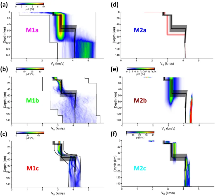
The inversion results of the six methods are displayed in Figure 11. They show the additional gain in infor-mation obtained through inversion, compared to the prior distributions (Figure 8). The thick black line represents the 1‐D base model used to compute the synthetic seismograms, whereas the gray area shows the minimum and maximum VSvalues encountered over the great circle path between source and receiver.
The inverted data sets are the body waves and surfaces waves arrival times estimated by the MQS (Table 1 and Figures 1 and 5), except for the M1b and M1c methods, which use group velocity dispersion diagrams (Figure 6) and both waveforms and group velocities, respectively. The data fit is shown in Figure 12. Figure 11 clearly highlights the nonuniqueness of the solution. Depending on the depth, some distributions are unimodal, bimodal, or multimodal. The results show that none of the distributions perfectlyfit the input model, but depending on the method, they share some common feature with the model to retrieve. Let usfirst review the results of the three M1 methods. The pdf of the M1a method (Figure 11a) is spread within the parameter space, because both the seismic velocity profiles and the quake location are simulta-neously inverted, with relatively large prior bounds. The maximum of the pdf between 15‐ and 70‐km depth is located in the vicinity of the input model, which means that VSin the crust is well constrained. Below
80‐km depth the distribution enlarges and has a similar shape to the a priori pdf (Figure 8a), which means that the sensitivity to the data decreases at these depths (the highest period of surface wave considered with this method is 40 s; Figure 12). The discontinuity located at 100‐km depth is due to the prior assumptions and the loss of sensitivity of surface waves at these depths. The pdf of M1b (Figure 11b), obtained using surface waves measurements only, is narrower compared to the previous method, mostly because the source loca-tion and the origin time arefixed to the MQS values. Although surface wave data are known to be less sen-sitive to the sharpness of the discontinuities, two inflexion points are observed near 15‐ and 60‐km depth, close to the two discontinuities of the input model. The VS distribution in the crust lies within the
minimum and maximum VSvalues encountered along thefirst orbit Rayleigh wave path. Similarly to the
M1a method, the pdf is spread below 70‐km depth. This enlargement is also visible on the results obtained with the M1c method (Figure 11c), which invert both surface wave group velocities and surface wave waveforms. The retrieved VSvalue in the crust is constant with depth, overestimated in the upper
crust and slightly underestimated in the lower crust, which means that the M1c inversion is unable to recover the detailed layering of the crust, which is not surprising considering the sensitivity of Rayleigh waves at the periods measured (between 25 and 55 s; Figure 12). The M1c pdf shows a discontinuity clearly located at 50‐km depth, in the range of the model to retrieve, because the crustal thickness is allow to slightly vary between ±4 km around the 50‐km‐thick crust 1‐D model chosen as the starting model of the inversion. The M1c method is also able to provide the strike, dip, slip, and the focal depth of the
Figure 11. Posterior probability density functions (pdf) of VSas a function of depth for M1 (a–c) and M2 (e–f) methods. Blue and red colors are low and high probability, respectively. Concerning the M2a method (d), the accepted models are shown in red. The black lines in (a) and (b) show the upper and lower prior bounds. The thick black line represents the 1‐D base model used to compute the synthetic seismograms, whereas the gray area shows the
marsquake. Figure 13 shows that the strike's distribution is centered near 110°, in agreement with the MQS values. In return, the focal depth is not constrained by the data, and changes in the marginal distributions for the dip, slip, and Moho depth indicates trade‐offs among the parameters.
By analyzing the output distributions of the M1 models, we conclude that (1) VSin the crust is relatively well
constrained and consistent to the mean path averaged values; (2) the structure is not reliably constrained below 70 km; (3) the crustal thickness is difficult to retrieved by inverting both the VSprofile and the quake
location (M1a), but it could be approximated if the quake location isfixed (M1b) or if small perturbations around a 1‐D starting model with a Moho depth already close to the model to retrieve are performed (M1c). Concerning the three methods handling geophysical and geodynamical parameters, VS in the crust is
slightly underestimated for M2a models (Figure 11d) and overestimated for M2c (Figure 11f). Note that
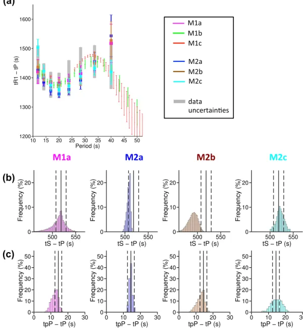
Figure 12. Fit of data for both Rayleigh and body waves. (a) The mean value and ± mean absolute deviation of the arrival time of Rayleigh waves minus the arrival times of P wave as a function of frequency, for all sampled models. The thick gray lines show the data uncertainties estimated by MQS. (b and c) The marginal probabilities of tS− tPand tpP− tP, respectively. Relative to the legend, colors are less vivid because profiles have been plotted using a
transparency factor. Note that the methods M1b and M1c do not used body waves. The black line and dashed lines show the arrival time and uncertainty measured by MQS.
the depth of the discontinuity between the upper crust and the lower crust of M2a models isfixed and not inverted during the inversion scheme. For the M2c models, higher VSvalues in the crust are explained by
the choice of the a priori distribution, showing low probabilities near the VSvalue to retrieve (Figure 8f).
Conversely, M2b modelsfit well the VSvalues in the lower crust (Figure 11e), because a large range of
values is considered (Figure 8e). Contrary to M1 models, M2 models provide a quantitative estimate of the Moho depth (Figure 14). For the M2a method, the largest number of models show a Moho located near 75‐km depth (Figure 14a), which is outside the range of Moho depths along the first orbit. The M2b a
Figure 13. Marginal probabilities of the strike, dip, slip, focal depth, and Moho depth obtained using the M1c method. The estimated values from MQS are shown in red, and the true values are in black. The a priori distribution is the gray area centered on the MQS value.
Figure 14. Marginal probabilities of the Moho depth for the three M2 methods. The black line show the Moho depth of the 1‐D base model, whereas the dashed red lines define the range of the crustal thickness along the R1 path. The a priori distributions are shown in gray.