MRSI data unmixing using spatial and spectral priors in transformed domains

O

pen

A

rchive

T

OULOUSE

A

rchive

O

uverte (

OATAO

)

OATAO is an open access repository that collects the work of Toulouse researchers and

makes it freely available over the web where possible.

This is an author-deposited version published in :

http://oatao.univ-toulouse.fr/

Eprints ID : 17095

The contribution was presented at ISBI 2016 :

http://biomedicalimaging.org/2016/

To cite this version :

Laruelo, Andrea and Chaari, Lotfi and Ken, Soleakhena

and Tourneret, Jean-Yves and Batatia, Hadj and Laprie, Anne MRSI data

unmixing using spatial and spectral priors in transformed domains. (2016) In:

13th IEEE International Symposium on Biomedical Imaging: From Nano to

Macro (ISBI 2016), 13 April 2016 - 16 April 2016 (Prague, Czech Republic).

Any correspondence concerning this service should be sent to the repository

administrator:

[email protected]

MRSI DATA UNMIXING USING SPATIAL AND SPECTRAL PRIORS IN TRANSFORMED

DOMAINS

A. Laruelo

, L. Chaari

, S. Ken

, J.-Y. Tourneret

, H. Batatia

and A. Laprie

1

_{Institut Claudius Regaud, Toulouse, F-31059 France}

_{Univ. of Toulouse, IRIT - INP-ENSEEIHT, France}

3

_{MIRACL Laboratory, Sfax, Tunisia}

4

_{Universit´e Toulouse III Paul Sabatier, Toulouse, F-31000 France}

ABSTRACT

In high-grade gliomas, the tumor boundaries and the degree of infiltration are difficult to define due to their heterogeneous composition and diffuse growth pattern. Magnetic Resonance Spectroscopic Imaging (MRSI) is a non-invasive technique able to provide information on brain tumor biology not avail-able from conventional anatomical imaging. In this paper we propose a blind source separation (BSS) algorithm for brain tissue classification and visualization of tumor spread using MRSI data. The proposed algorithm imposes relaxed non-negativity in the direct domain along with spatial-spectral regularizations in a transformed domain. The optimization problem is efficiently solved in a two-step approach using the concept of proximity operators. Vertex component anal-ysis (VCA) is proposed to estimate the number of sources. Comparisons with state-of-the-art BSS algorithms on in-vivo MRSI data show the efficiency of the proposed algorithm. The presented method provides patterns that can easily be re-lated to a specific tissue (normal, tumor, necrosis, hypoxia, edema or infiltration). Unlike other BSS methods dedicated to MRSI data, it can handle spectra with negative peaks and results are not sensitive to the initialization strategy. In addi-tion, it is robust against noisy or bad-quality spectra.

Index Terms— blind source separation (BSS), tissue pat-terns, MRSI

1. INTRODUCTION

Conventional magnetic resonance imaging (MRI) is widely used for the diagnosis and follow-up of brain tumors due to its ability to provide detailed information about brain structures. Nevertheless, MRI does not always have sufficient specificity to identify different pathological areas in heterogeneous brain tumors. For instance, tumor infiltration into the normal tissue cannot always be differentiated from edema on T2-weighted or fluid-attenuated inversion recovery (FLAIR) images. MR spectroscopic imaging (MRSI) helps to overcome this limita-tion as it is able to characterize biochemical changes in brain tissues before they become visible in conventional MRI [1]. Supervised methods relying on known spectral models have been widely used to discriminate between tissue types.

How-ever, the outcome of these methods strongly depends on the prior knowledge considered and on the algorithm used [2]. In addition, supervised pattern recognition methods require a large number of expert-labeled spectra which are not al-ways available. Blind source separation (BSS) techniques appear as an interesting alternative for the analysis of MRSI data as they allow to estimate the sources and their abun-dances without (or with very little) prior knowledge. Differ-ent BSS methods have been proposed in the context of neuro-oncology to distinguish normal from abnormal spectra. Most of these methods are variants of the well-known non-negative matrix factorization (NMF) algorithm [3]. Sajda et al. [4] pro-posed a constrained non-negative matrix factorization method to extract physically meaningful tissue patterns from long-echo time (TE) MRSI data. Ortega-Martorel et al. [5] used convex NMF for brain tumor delineation on pre-clinical data. Li et al. [6] introduced a hierarchical NMF method able to identify normal, tumor and necrosis tissues in glioblastoma (GBM) patients. All these methods are heavily dependent on the initialization values and/or require the sources to be non-negative. The use of non-negative sources can be a clear lim-itation for the analysis of MRSI data given that MR spectra can take negative values (such as the inverted lactate peak for long-TE data.)

Recently, BSS methods exploiting not only the spectral but also the spatial context of the signals have been proposed [7]. These algorithms incorporate spatial priors based on smooth spatial variations or on the sparsity of the abundance matrix. In this paper we describe a method which jointly incorporates prior knowledge about the spatial and spectral dimensions of MRSI data. The originality of this method lies in the combi-nation of spectral and spatial priors in a transformed domain into a spectral unmixing procedure, as well as the control of the non-negativity constraint for the sources. It aims at in-creasing the signal-to-noise ratio (SNR) of the data and to favor solutions with few irregularities in the spatial and the spectral dimensions. The proposed method is able to extract more than two physically meaningful tissue patterns and it is not restricted to non-negative sources. In addition, the results do not depend on the initialization strategy since this

algo-rithm relies on the optimization of convex functions. Further-more, it is robust to noise and to the presence of low quality spectra.

2. BLIND SOURCE SEPARATION METHOD BSS methods assume that the measurements (spectra) can be expressed as linear mixtures of sources plus some noise. This can be expressed in matrix form as follows:

Y _{= SA + N} (1)

where Y is the data matrix in which each column is a mea-surement (spectrum), S is the unknown source matrix in which each column is a source, A is the unknown mixing matrix which defines the contribution (abundance) of each source in each spatial position (voxel) and N is the unknown noise matrix accounting for instrumental noise and/or model imperfections.

BSS methods aim at estimating both A and S from the mea-sured data Y . Under the assumption of independent and identically distributed (i.i.d.) Gaussian noise, the maximum-likelihood estimator is defined by the standard problem:

arg min S,A 1 2kY − SAk 2 2 (2)

The problem (2) is ill-posed in the sense that it has an infinite number of solutions and that there is no analytical method to identify them. In order to find an optimal solution of (2) it is standard to constrain A and/or S to privilege solutions with desired properties. These constraints can be seen as prior information injected in the resolution of (2). The following sections describe the priors used in this paper.

2.1. Spectral prior

In many applications, sources are considered sparse as for the case for MRSI spectra. In the wide sense, a sparse signal is a signal that can be expressed with only a few large non-zero coefficients, or can be well approximated in such a way. The sparsity of the sources can be enforced by constraining their ℓ1norm as follows: arg min S,A 1 2kY − SAk 2 2+ α1kSk1 (3)

where α1 ∈ R+controls the trade-off between data fidelity

and prior information. In order to better model this kind of signals, one can express them in a different domain where the sparsity is more noticeable. In this paper, we exploit the fact that the sources are sparse in the wavelet domain leading to the following problem:

arg min S,A 1 2kY − SAk 2 2+ α1kT Sk1 (4)

where T is a dyadic 1D orthonormal wavelet decomposition operator.

2.2. Spatial prior

Recently, it has been proposed to exploit not only the spec-tral, but also the spatial context of the signals by incorporat-ing spatial priors. Previous approaches favor smooth spatial variations or spatially structured sparsity by imposing appro-priate constraints on the mixing-matrix A [7]. We propose in this paper a novel spatial prior which, together with the spec-tral term, increases the signal-to-noise ratio (SNR) of the data and exploits the neighbouring information along the spatial dimension for a given MRSI voxel. The proposed criterion to be minimized can be written as follows:

arg min S,A 1 2kY − SAk 2 2+ α1kT Sk1+ α2 M X m=1 kF (SA)m_k 1 (5) where α2∈ R+is the regularization parameter of the spatial

prior information, m = 1, ..., M is the spectral frequency, (SA)m_{is the 2D image which results from reshaping the mth}

column of SA and F is a dyadic 2D orthonormal wavelet decomposition operator.

2.3. Non-negativity constraints

The entries of both the abundances A and the sources S are often assumed to be non-negative. This is always true for A since the mixture coefficients are function of the relative con-centrations of the observed physical entities, which are neces-sarily non-negative. However the non-negativity assumption does not always hold for MRSI spectra that may include neg-ative peaks (as it is the case of the inverted lactate peak for long-TE MRSI data). BSS methods based on NMF are lim-ited to use absolute or truncated spectra (negative values set to zero). In order to avoid this limitation, we propose to re-lax the non-negativity constraint for the matrix of extracted sources as follows: arg min S,A 1 2kY − SAk 2 2+ α1kT Sk1+ α2 M X m=1 kF (SA)m_k 1 + i+ (A) + α3i+(S) (6)

where i+is the indicator function on[0, ∞) and α3 ∈ [0, 1]

allows the relaxation of the non-negativity constraint of the sources.

2.4. Optimization procedure

The minimization of the objective function (6) can be car-ried out solving alternately the convex subproblems with respect to A and S. However the objective functions of both sub-problems are not differentiable, which prevents the use of standard gradient-based algorithms for minimization. We therefore propose to perform the minimization by us-ing the concept of proximity operators [8] which was found to be fruitful in a number of recent works in convex opti-mization [9]. We propose to solve the marginal problem in S by using the Generalized Forward-Backward (GFB) al-gorithm [10]. The minimization with respect to A can be

solved using the simultaneous direction method of multipli-ers (SDMM) described in [11]. The alternating updates are then repeated for a number of iterations (Algorithm 1). Algorithm 1 BSS Algorithm

Set N, T, F, α1, α2, α3 Set NbSources= V CA(Y )

Set Ak= abs(randn(NbSources, NbSpectra)) for iter= 1 to N do

Set piA= pinv(Ak) Set Sk= Y ∗ piA

Calculate Sk= GF B(Y , Ak, Sk, T, α1, α3) Calculate Ak= SDM M (Y , Ak, Sk, F, α2) end for

return S= Sk Normalize columns of Ak. return A= Ak

3. RESULTS

We have tested the proposed method on in-vivo MRSI data from 10 patients with newly diagnosed GBM included in a prospective clinical trial. We show the results for three repre-sentative cases: identification of intratumoral necrotic areas, discrimination of necrosis and hypoxia and detection of tu-mor infiltration. Data were acquired with a Siemens Avanto 1.5 T using a 3D CSI sequence with water suppression, echo time (TE) of 135 ms, repetition time (TR) of 1500 ms, 512 data points and 4 averages. We have used Vertex Compo-nent Analysis (VCA) [12] to estimate the number of sources. Highly correlated sources (Pearson’s correlation coefficient (ρ) higher than 0.8) were automatically discarded. A was initialized as the absolute value of an i.i.d. Gaussian random matrix. The values of the spatial and the spectral regulariza-tion parameters of the objective funcregulariza-tion (6) were estimated by cross validation and set to α1 = 0.05 and α2 = 0.1. The

wavelets used in these experiments were Daubechies (db2). Fig. 1 shows a comparison of the proposed method (SSR) with two other state-of-the-art BSS methods, HALS [13] and sparse NMF (SNMF) [7]. Both algorithms have been run us-ing the default parameters. In order to show the improve-ment due to the incorporation of the spatial term, the results obtained when only the sparsity of the sources is considered (α1= 0.05 and α2= 0 in (6)) are also displayed and referred

to as SSR-Spectro. While HALS and SNMF are able to ex-tract only two physically meaningful sources, SSR is able to detect three sources (normal (j), tumor (k) and necrosis (l) in Fig. 1) that are in agreement with the companion MRI im-age. Note that the abundance maps correspond to the voxels within the volume of interest (VOI), i.e., the inner 10 × 10 grid inside the white rectangle. Among the compared meth-ods, SSR is the only one capable of identifying the necrosis area even when only the spectral prior is considered (SSR-Spectro). However, by adding the spatial term, the identifi-cation of the tumor and necrosis regions is clearly improved and the sources are less correlated (mean ρ is 0.65 for SSR and 0.74 for SSR-Spectro) and therefore more easily inter-pretable than the sources obtained with SSR-Spectro. For this

comparison we have used magnitude spectra since HALS and SNMF (NMF-based methods) are restricted to non-negative sources. This can be a clear limitation because different tissue patterns may present similar magnitude spectra. For example, the presence of lactate (marker of hypoxia) and lipids (indi-cating the presence of necrosis) are of high diagnostic value because these metabolites are not detectable in healthy brain tissue. However, in (long-TE) MRSI spectra the inverted peak of lactate occupies the same resonant frequency as lipid, and both metabolites are difficult to differentiate when using mag-nitude spectra. Fig. 2 shows the results provided by the pro-posed method using the real part of the spectra for an MRSI dataset presenting hypoxic and necrotic tumor regions. The predominant pattern (g) corresponds to spectra with normal levels of choline (Cho), creatine (Cr) and N-acetyl-aspartate (NAA) and presence of lactate (Lac) throughout the FLAIR-enhanced area (c). SSR is able to differentiate two different tumor patterns, the necrotic core (h) (high Cho, low NAA and presence of lipids) and a hypoxic area (i) (high Cho, low NAA and presence of Lac). In addition, the proposed method is ro-bust against the presence of bad quality spectra, which are grouped in a separated pattern. This is the case of the fourth source (j) that represents spectra where the NAA signal is obscured due to a severe lipid contamination. Fig. 3 shows that the proposed method is also able to differentiate between tumor infiltration and edema in peri-enhancing oedematous-appearing areas. Discriminating between these two cases is not always possible from FLAIR (or T2-weighted) images. Edema (g) does not modify metabolic ratios (j) whereas tu-mor infiltration (f) shows a pattern with increased Cho and decreased NAA (i). The pattern of edema (j) shows reduced metabolite peaks possibly due to the the presence of intersti-tial water that decreases the signal of the metabolites [14]. The presence of Lac and decreased NAA are also in accor-dance with cerebral peritumoral edema [15]. The map of tu-mor infiltration (f) is in accordance with the later relapse of the patient (d).

Fig. 1: Left: Maps showing the spatial distribution of the different tissue patterns (sources). Middle: sources related to normal tissue (a, d, g, j), tumor (b, e, h, k) and necrosis (c, f, i, l). Right: T1-weighted after gadolinium injection (top), voxels within the volume of interest (bottom).

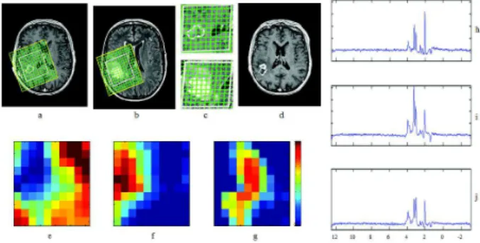
Fig. 2: T1-weighted after gadolinium injection (left) and voxels within the volume of interest (right) (a); FLAIR (left) and voxels within the volume of interest (right) (b); Maps showing the spatial distribution of normal tissue (c), necrosis (d), hypoxia (e) and lipid contamination (f); Sources related to normal tissue (g), necrosis (h), hypoxia (i) and lipid contamination (j).

Fig. 3: T1-weighted after gadolinium injection and FLAIR images before treatment (a) and (b); corresponding voxels within the volume of interest (c); T1-weighted after gadolinium injection at relapse (d); Maps showing the spatial distribution of normal tissue (e), tumor infiltration (f) and edema (g); Sources related to normal tissue (h), tumor infiltration (i) and edema (j).

4. CONCLUSION

We presented a new blind source separation method which combines spatial and spectral regularizations in the wavelet domain. The method exploits magnetic resonance spectro-scopic imaging data properties such as the sparsity of the spectra in the wavelet domain and the spatial regularity be-tween neighbouring voxels. Experiments on in-vivo data show that the proposed method is able to extract more than two physically meaningful tissue patterns easily interpretable. The abundance maps show spatially coherent and well de-fined areas, in agreement with expert assesment conducted on companion anatomical MRI images. Unlike previous ex-isting methods, the proposed strategy can deal with negative sources and is not sensitive to initialization. In addition it is robust against noise and the presence of low quality spectra. Future work includes a consistency analysis of the proposed method for a larger group of patients.

5. ACKNOWLEDGMENTS

This work is part of the SUMMER Marie Curie Research Training Net-work (PITN-GA-2011- 290148), which is funded by the 7th FrameNet-work Pro-gramme of the European Commission (FP7-PEOPLE-2011-ITN). The infor-mation and views set out in this publication are those of the authors and do

not necessarily reflect the official opinion of the European Union. Neither the European Union institutions and bodies nor any person acting on their behalf may be held responsible for the use which may be made of the information contained therein.

6. REFERENCES

[1] A. Deviers, S. Ken, T. Filleron, B. Rowland, A. Laruelo, I. Catalaa, V. Lubrano, P. Celsis, I. Berry I, G. Mogicato, E. Cohen-Jonathan Moyal, and A. Laprie, “Evaluation of lactate/Nacetylaspartate ratio deffined with MR spectroscopic imaging before radiotherapy as a new predictive marker of the site of relapse in patients with glioblastoma multiforme,” Int. J. Radiat. Oncol. Biol. Phys., vol. 90(2), pp. 385– 393, 2014.

[2] E. Mosconi, D. M. Sima, M. I. Osorio Garcia, M. Fontanella, S. Fiorini, S. Van Huffel, and P. Marzola, “Different quantification algorithms may lead to different results: a comparison using proton MRS lipids signals,” NMR Biomed., vol. 27(4), pp. 431–443, April 2014. [3] D. D. Lee and H. S. Seung, “Learning the parts of objects by

non-negative matrix factorization,” Nature, vol. 401, pp. 788791, 1999. [4] P. Sajda, S. Du, T. R. Brown, R. Stoyanova, D. C. Shungu, X. Mao,

and L. C. Parra, “Nonnegative matrix factorization for rapid recovery of constituent spectra in magnetic resonance chemical shift imaging of the brain,” IEEE Trans. Med. Imaging, vol. 23, pp. 1453–1465, 2004. [5] S. Ortega-Martorell, P. J. G. Lisboa, A. Vellido, R. V. Sim oes,

M. Pumarola, M. Juli`a-Sap´e, and C. Ar´us, “Convex Non-Negative Matrix Factorization for Brain Tumor Delimitation from MRSI Data,” PLoS ONE, vol. 7(10), 2012.

[6] Y. Li, D. M. Sima, S. V. Cauter, A. R. Croitor Sava, U. Himmelreich, Y. Pi, and S. Van Huffel, “Hierarchical non-negative matrix factoriza-tion (hNMF): a tissue pattern differentiafactoriza-tion method for glioblastoma multiforme diagnosis using MRSI,” NMR Biomed., vol. 26(3), pp. 307– 319, 2013.

[7] N. Gillis and R. J. Plemmons, “Sparse Nonnegative Matrix Under-approximation and its Application for Hyperspectral Image Analysis,” Linear Algebra and its Applications, vol. 438(10), pp. 3991–4007, 2012.

[8] J. J. Moreau, “Proximit´e et dualit´e dans un espace hilbertien,” Bulletin de la Socit´e Math´ematique de France, vol. 93, pp. 273–299, 1965. [9] L. Chaari, J.-C. Pesquet, A. Benazza-Benyahia, and P. Ciuciu, “A

wavelet-based regularized reconstruction algorithm for SENSE paral-lel MRI with applications to neuroimaging,” Med. Image Anal., vol. 15, no. 2, pp. 185–201, 2011.

[10] J. Fadili H. Raguet and G. Peyr´e, “A Generalized Forward-Backward Splitting,” SIAM Journal on Imaging Sciences, vol. 6, pp. 11991226, 2013.

[11] P. L. Combettes and J. C. Pesquet, “A proximal decomposition method for solving convex variational inverse problems,” Inverse Problems, vol. 24(6), 2008.

[12] J. M. P. Nascimento and J. M. Bioucas Dias, “Vertex component anal-ysis: a fast algorithm to unmix hyperspectral data,” IEEE Transactions on Geoscience and Remote Sensing, vol. 43(4), pp. 898–910, 2005. [13] N. Gillis and F. Glineur, “Accelerated Multiplicative Updates and

Hier-archical ALS Algorithms for Nonnegative Matrix Factorization,” Neu-ral Computation, vol. 24(4), pp. 1085–1105, 2012.

[14] A. Di Costanzo, F. Trojsi, M. Tosetti, G. M. Giannatempo, F. Nemore, M. Piccirillo, S. Bonavita, G. Tedeschi, and T. Scarabino, “High-field proton MRS of human brain,” Eur J Radiol, vol. 48, pp. 146153, 2003. [15] R. Riccia, A. Baccia, V. Tugnolib, S. Battagliaa, M. Maffeia, R. Agatia, and M. Leonardia, “Metabolic Findings on 3T 1H-MR Spectroscopy in Peritumoral Brain Edema,” AJNR, vol. 28, pp. 1287–1291, 2007.