Université de Liège Faculté des Sciences
Département des Sciences et Gestion de l’Environnement
Assessment of fodder biomass in Senegalese rangelands using earth
observation and field data
Abdoul Aziz DIOUF Thèse présentée en vue de l’obtention du grade de Docteur en Sciences Octobre 2016
Composition du jury :
Président : Dr Pierre OZER (ULg) Promoteur : Pr Bernard Tychon (ULg)
Co-promoteur : Dr, HDR, Jacques André NDIONE (CSE) Lecteurs : Dr Bakary Djaby (AGRHYMET)
Pr Jos Van Orshoven (KU Leuven) Dr Pierre Hiernaux (GET)
Dr Joost Wellens (ULg)
Université de Liège Faculté des Sciences
Département des Sciences et Gestion de l’Environnement
Assessment of fodder biomass in Senegalese rangelands using earth
observation and field data
Abdoul Aziz DIOUF Thèse présentée en vue de l’obtention du grade de Docteur en Sciences Octobre 2016
Composition du jury :
Président : Dr Pierre OZER (ULg) Promoteur : Pr Bernard Tychon (ULg)
Co-promoteur : Dr, HDR, Jacques André NDIONE (CSE) Lecteurs : Dr Bakary Djaby (AGRHYMET)
Pr Jos Van Orshoven (KU Leuven) Dr Pierre Hiernaux (GET)
To my late father Abdoulaye Diouf; To my mother, Aïssatou Diouf; To my wife, Khady Diouf; And to you;
Acknowledgments
My first thanks go to the members of my thesis committee who framed and followed my work, and who have given me support and encouragement throughout this long and beautiful adventure. Thank you to Bernard Tychon, promoter of this thesis, for the trust he has given me from the beginning of my research and for his promptness to answer my queries both scientifically and administratively. Thank you to Bakary Djaby, who guided my first steps in the use of statistical tools and the modelling. Thank you to Jacques André Ndione, co-advisor of this thesis, for being always available to read and reread my search results from Dakar to Lome, but also for giving me valuable advices which have contributed to the completion of this work and that is now "ma tasse de Kinkeliba" ...
Thank you to the General Direction of the Centre de Suivi Ecologique (CSE), especially Assize Touré, General Director, Amadou Moctar Dièye, Technical director and Oumar Sarr, Administrative and Financial director, for their trust to me and for allowing me to do this thesis. Thank you to the AGRICAB project managers and experts at the Flemish Institute for Technological Research (VITO), the CSE and the University of Liège (ULg): Tim Jacobs, Carolien Tote, Mouhamadou Bamba Diop (“segn bi”, especial thanks to you for all), Antoine Royer (many thanks to you for contributing vastly to my knowledge in remote sensing) and Julien Minet, for making all this research possible.
Thank you to the members of the jury for the time, interest and constructive comments you have made to this dissertation.
Many thanks go to Abdoulaye Wélé, Aliou Diouf, Moussa Dramé, Moussa Sall, Aliou Ka, Gora Bèye and Ibrahima Diop etc., not forgot all car-drivers and other field assistants, who helped to collect ground data from 1999 to 2015. Without your support this work would not have been possible.
Thank you to my co-authors of the publications: Martin Brandt, Aleixandre Verger, Moussa El Jarroudi, Bakary Djaby, Rasmus Fensholt, Jacques André Ndione, Bernard Tychon, Mouhamadou Bamba Diop,
the beginning to have my first peer reviewed publication in Remote Sensing. He also made a remarkable contribution to the design of my work, from the codes shared to the proofreading of the dissertation.
Thank you to the Rasmus’s team at Department of Geosciences and Natural Resource Management of the University of Copenhagen (not to mention names) for the hospitality during my visit over there in May 2016, the time and the valuable remarks they have made on the first draft of this dissertation. Thanks also to Stefanie M. Herrmann.
Thank you to all colleagues at CSE for the valuable advice and encouragement along this research: special thanks to Taibou Ba, who has been the first to identify me as a good candidate for this thesis by informing me about the proposal. Further thanks go to my office colleague, Marième Diagne and his twins (Fatou Binetou Traore and Batouly Ly). Thanks to the lunch break team, "wa ministère de la santé or wa daradji" for the good times spent together around the meals.
Thank you to all colleagues of the Department of Science and Environment Management (at the Arlon Campus Environment of ULg): especially to the "BT" team, Moussa El Jarroudi, Joost Wellens, Abdoul Hamid Mouhamed Sallah, Marie Lang, Antoine Denis, Sie Pale, Julien Minet, Claire Simonis, Ingrid Jacquemin, Mahamadou Karimou Barke, for their sense of humor (soupé les "jeudredis" soir), and for discussions about science and everyday life during coffee-breaks. Especial thanks to Tarik Ben Abdelouahab for all. Thanks also to Farid Traore for guiding my first steps across the Arlon's city and for advising me about PhD requirements, and to Louis Kouadio Amani for sharing useful statistical codes. Thanks go to Catherine Heyman for its assistance each time I was planning a travel to Belgium. Thanks to the running team (FulguRUN!!!) of the campus, for the good time we spent together during the rally "year 199th of the ULg": I'll be happy to run next year again for the bicentenary of the University...
Many thanks to the Senegalese community in Arlon, especially to Idrissa, Mame Fatou, Ka Rokhaya and Ka Maïmouna for all wonderful things they have done for me. I do not forget Insa Goudiaby and Pape Diouf and their families.
Thank you to managers and godparents of the Non-Governmental Organization “JUDDU” which help children from poor families in Pikine (Senegal) to have a better education. Especial thanks to Cathy Le Baron, Jean Francois Blérot and Françoise Poullet Blérot for effort they are spending for “JUDDU”, and for encouragement and nice moments we shared in Belgium.
Thank you to the European Union which funded the AGRICAB project (282621) within the seventh Framework Programme (FP7). Thanks also to the European Earth observation programme, Copernicus Global Land and the GIOBIO (32-566) project for providing the satellite imagery at no cost. Thank you to the USGS Earth Resources Observation and Science Center (EROS) and the Famine Early Warning Systems Network (FEWS NET) Project for providing satellite imagery and the GeoWRSI software. Many thanks to the “Académie de Recherche et d’Enseignement Supérieur (ARES)” and the “Centre pour le Partenariat et la Coopération au Développement (PACODEL)” of the University of Liège for the fellowship allocated for the completion of this thesis.
Finally, this work would not have been completed without the support and encouragement of my friends, my parents and my wife to whom I further say thank you.
Summary
Senegalese livestock size has largely increased during the last three decades in relation to the population growth. The fodder biomass stock available at the end of the growing season, therefore, becomes increasingly limited to meet feeding needs of pastoral livestock which provides third of the national agricultural wealth. With the reduction of natural grazing lands mostly generated by the expansion of croplands, and the reduction of fodder biomass production due to drought effects, the increase of the livestock size leads to the rangelands overload whose persistence can lead in turn to their degradation. A technique based on a simple linear relationship between the temporal integration of the Normalized Difference Vegetation Index (NDVI) and the ground biomass data, developed in the 1980s, has been operationally applied by the Centre de Suivi Ecologique (CSE) of Dakar (Senegal) to assess the fodder biomass available in rangelands at the end of the growing season. The derived map of total biomass production enables to help pastoral livestock managers as well as national stakeholders against food insecurity and natural resources degradation. Carried out annually, this approach comprises unfortunately some uncertainties as: (1) the saturation drawback of NDVI in areas with high biomass productivity, (2) the temporal scale which is restricted to biomass data of the ongoing year not being used again in the following year, (3) the low predictive ability due to the large time gap between data collection and published results, and (4) the high costs for annual data collection. In addition, although the earth observation (EO) data have largely progressed during the last three decades, this technique has not changed over this period and consequently is not state-of-the-art. To tackle these limitations and advance the traditional method, new statistical models that include new earth observations datasets and historical in situ plant biomass data were developed for estimating and / or predicting the forage availability at the end of the growing season in Senegalese semi-arid rangelands. A backward analysis of the linear regression approach currently applied in Senegal provided evidence that nonlinear regression functions such as Exponential and Power are more suited to estimate the end-of-season total biomass in this region using annual data solely. A completely new methodology using multiple-linear models which include various
phenological metrics from the time series of the Fraction of Absorbed Photosynthetically Active Radiation (FAPAR) and 14 years of in situ total biomass samples was developed. The proposed approach provided more reliable and accurate estimates as compared to the current CSE biomass product. Multiple-linear models developed with specific metrics adapted to ecosystem properties increased the overall accuracy of the fodder biomass estimates and mitigated the saturation of FAPAR obtained with models run across the whole study area. With this new approach, timely information about possible deficits/surplus of total fodder biomass can be provided to stakeholders using phenological metrics that are available relatively early in the growing season. Another new approach based on a machine learning algorithm (i.e., Cubist) was developed, as never done before, to assess herbaceous biomass in Senegalese Sahel. Three Cubist models using FAPAR seasonal metrics and/or agrometeorological variables (i.e., soil water status indicators) were established and compared. The Cubist model including both FAPAR and agrometeorological variables provided the best estimation performance. This model enabled to mitigate the saturation affecting optical remotely sensed vegetation data in areas of high plant productivity as well as the discrepancy between herbaceous biomass and greenness, and corrected therefore for herbaceous biomass underestimations observed with the sole FAPAR based model, particularly in sparsely vegetated areas. In contrast to the date of the growing season onset retrieved from FAPAR seasonal dynamics, the rainy season onset was significantly related to the herbaceous biomass and its inclusion in models could constitute a significant improvement in forecasting risks of fodder biomass deficit. The methods developed in this research provide tools to assess Senegalese forage resources at two levels: herbaceous and total fodder biomass (Herbaceous + woody leaf biomass). They require limited data and free available software and therefore can be easily replicated in other countries of the West African Sahel.
Keywords: fodder biomass, models, FAPAR, phenological metrics, growing season, herbaceous, forecast, food security, Senegal, Sahel.
Résumé
La taille du cheptel sénégalais a connu une forte augmentation au cours des trois dernières décennies en relation avec la poussée démographique. La production fourragère en fin de saison se rapproche de plus en plus des limites de satisfaction des besoins alimentaires du cheptel essentiellement pastoral qui fournit le tiers de la richesse agricole nationale. Avec la réduction des parcours naturels liée globalement à l’augmentation des terres de culture, et la réduction de la production de biomasse causée par la sécheresse, l’accroissement du cheptel entraine une surcharge des parcours, dont la persistance conduit à leur dégradation. Afin d’estimer le disponible fourrager des parcours à la fin de la saison de croissance, le Centre de Suivi Ecologique (CSE) de Dakar applique de manière opérationnelle, une technique utilisant une régression linéaire simple entre l’indice de végétation NDVI (Normalized Difference Vegetation Index) cumulé au cours de la saison et les données de biomasse végétale collectées sur le terrain. La carte de production fourragère élaborée annuellement est très utile pour les gestionnaires du système pastoral ainsi que les décideurs nationaux en matière de lutte contre l’insécurité alimentaire et la dégradation des ressources naturelles. Malheureusement, cette technique comporte un certain nombre de contraintes liées à : (1) la saturation du NDVI dans les zones à forte production fourragère, (2) les données de biomasse limitées à l’année en cours et qui ne sont pas utilisées les années suivantes, (3) la faible capacité de prévision en raison du temps important entre la collecte des données sur le terrain et la publication des résultats, et (4) le coût élevé requis pour la collecte annuelle des données. Par ailleurs, bien que les données d’observation de la terre (satellitaires) aient largement évolué au cours des trois dernières décennies, cette technique n’a pas changé et reste à améliorer par rapport à l’état de l’art actuel. Afin d’améliorer cette méthode « traditionnelle », de nouvelles approches statistiques ont été proposées dans cette étude. Ces méthodes intègrent de nouvelles données d’observation de la terre et des données historiques de production fourragère pour estimer et/ou prévoir les quantités de fourrages disponibles à la fin de la saison au niveau des parcours du Sénégal. Une analyse comparative de l’approche par régression simple actuellement utilisée au Sénégal, a montré que les
fonctions non-linéaires, Exponentiel et Puissance sont plus adaptées à l’estimation du disponible fourrager de fin de saison en utilisant les données d’une seule année. Une approche entièrement nouvelle avec des modèles de régression multilinéaire a été développée. Elle utilise différentes métriques saisonnières issues de séries chronologiques de la fraction absorbée du rayonnement photosynthétiquement actif (FAPAR ou Fraction of Absorbed Photosynthetically Active Radiation) et 14 ans de données de biomasse fourragère totale. Cette approche fournit des estimations plus précises telles que comparées avec les sorties de la méthode du CSE. Les modèles de régression multiple développés avec des métriques saisonnières spécifiques et adaptées aux propriétés des écosystèmes ont permis d’améliorer la précision globale des estimations de la biomasse fourragère totale mais aussi d’atténuer la légère saturation du FAPAR observée avec les modèles appliqués à l’échelle de la zone d’étude. Avec cette nouvelle approche, l’information sur les déficits/surplus de biomasse fourragère totale peut être très tôt transmise aux décideurs en utilisant des variables saisonnières du FAPAR disponibles relativement tôt au cours de la saison de croissance. Une autre approche incluant un algorithme d’apprentissage automatique appelé Cubist, a été développée pour l’estimation de la biomasse fourragère herbacée au Sénégal. Trois modèles Cubist qui utilisent des métriques saisonnières du FAPAR et/ou des variables agrométéorologiques (indicateurs de l’état de l’eau dans le sol), ont été développés et comparés. Le modèle Cubist qui utilise à la fois les métriques du FAPAR et les variables agrométéorologiques, s’est montré plus performant. Ce modèle a permis d’atténuer la saturation qui caractérise les données de télédétection optique de la végétation dans les zones à forte densité végétale mais aussi, de réduire la différence souvent observée entre la masse de végétation herbacée et la valeur dérivée des indices satellitaires. Par conséquent, elle a permis de corriger la sous-estimation de la production de biomasse notée avec le modèle utilisant le FAPAR uniquement, particulièrement dans les zones à faibles couvert végétal. Contrairement à la date de démarrage de la saison de croissance calculée à partir du FAPAR, celle du démarrage de la saison des
déficits fourragers. Les méthodes développées dans cette étude constituent des outils d’estimation des ressources fourragères du Sénégal à deux niveaux : herbacé et total (herbacé et ligneux). Elles font appel à un nombre réduit de données et à des logiciels disponibles gratuitement, et donc peuvent facilement être reproduites dans d’autres pays du Sahel Ouest Africain.
Mots-clés : Biomasse fourragère, modèles, FAPAR, métrique, saison de croissance, herbacé, prévision, sécurité alimentaire, Sénégal, Sahel.
Abbreviations and Symbols
AET Actual EvapoTranspirationAGRHYMET Centre régional de formation et d'applications agronomique, hydrologique et météorologique
AGRICAB Agriculture Capacity Building AIC Akaike Information Criterion
AMMA Analyse Multidisciplinaire de la Mousson Africaine AMSU Advanced Microwave Sounding Unit
ANNs Artificial Neural Networks
APAR Absorbed Photosynthetically Active Radiation (MJ.m-2) ARC African Rainfall Climatology
AVHRR Advanced Very High Resolution Radiometer BS Bootstrap Sample
C Circumference (cm)
CART Classification And Regression Tree CCD Cold Cloud Duration
CESBIO Centre d’Etudes Spatiales de la BIOsphère CFS Committee on World Food Security
CILSS Comité inter-États de lutte contre la sécheresse au Sahel CPC Climate Prediction Center
CSE Centre de Suivi Ecologique CSWB Crop Specific Water Balance CV Coefficient of variation
DMP Dry Matter Productivity ECOeast Ferruginous Pastoral Region ECOnorth Northern Sandy Pastoral Region ECOsouth Eastern Transition Region
ECOwest Mixed Pastoral-Agricultural Region ENVISAT ENVIronment SATellite
EO Earth Observation EOS End Of Season
EOSp End Of Season from rainfall
ETm Maximum evapotranspiration in the decadal period EWS Early Warning Systems
FEWS Net Famine Early Warning Systems Network
fr Relative frequency of the stratum along the transect GCOS Global Climate Observing System
GEOV1 Geoland Version 1
GeoWRSI Geo-spatial Water Resource Satisfaction Index GPP Gross primary production (g.m-2)
HAPEX Hydrologic Atmospheric Pilot Experiment ILCA International Livestock Centre for Africa ILRI International Livestock Research Institute ISRA Institut Sénégalais de Recherches Agricoles Kc Crop coefficient
LAC Local Area Coverage LAI Leaf Area Index LOS Length Of Season LUE Light Use Efficiency MAE Mean Absolute Error METOP Meteorological Operational
MODIS Moderate Resolution Imaging Spectroradiometer ms Dry matter rate (%)
Mse Dry matter rate (%)
MSG Meteosat Second Generation MVC Maximum Value Composite
NDVI Normalized Difference Vegetation Index iNDVI Seasonal integrated of NDVI
NDVIpk Seasonal peak value of NDVI NGOs Non-Governmental Organizations
NIR Near-infrared portion of the electromagnetic spectrum (%) NMAE Normalized Mean Absolute Error
k-NN k-Nearest Neighbors
NOAA National Oceanic and Atmospheric Administration NPP Net primary production (g.m-2)
OLCI Ocean and Land Color Instrument OLS Ordinary Least-Squares
PAR Photosnthetically Active Radiation received by the canopy (MJ.m-2) PAW Plant Available Water
Pe Primary foliage production of one species (kg) PET Potential Evapotranspiration
Pf Foliar production (kg·DM.ha−1)
Ph Herbaceous dry matter production (kg·DM.ha−1) Pi Primary foliage production (kg)
PLS Partial Least Squares
pm Average green weight (g·m−2) PM Passive Microwave
PPT Annual Rainfall Amount
PROBA-V Project for On-Board Autonomy-Vegetation
Ps0 Standard average dry weight of foliar biomass of 10 twigs (kg) Pve Average weight of fresh foliar biomass of 10 twigs (kg) R Red portion of the electromagnetic spectrum (%) R² Coefficient of determination
RD Root Depth
RF Random Forest
RFE Rainfall Estimate
RG Global Radiation (MJ.m-2) RMSE Root Mean Square Error
RPCA Réseau de prévention des crises alimentaires
S Total area of four sampling plots (ha) SD Standard Deviation
SG Savitzky-Golay SOS Start Of Season
SOSp Start Of Season from rainfall
SPIRITS Software for the Processing and Interpretation of. Remotely sensed Image Time Series
SPOT Satellite Pour l’Observation de la Terre SSM/I Special Sensor Microwave Imager
STEP Sahelian Evaporation Transpiration and Production SW Soil Water Content
SWC Soil Water Level
TAMSAT Tropical Applications of Meteorology using SATellite
TIMESAT Software package to analyse time-series of satellite sensor data TIR Thermal infrared
ULg Université de Liège
VIP Variable Importance in the Projection VIs Vegetation Indices
VITO Flemish Institute for Technological Research V-test Wilcoxon signed rank test
Wd Amount of water stored in the soil at the end of the dekad Wd–1 Amount of water stored in the soil at the end of previous dekad WDEF Water Deficit
WHC Water Holding Capacity
WP Work Package
WRSI Water Requirement Satisfaction Index WSUR Water Surplus
WWF World Wide Fund
Ԑ Environmental stress scalar
Ԑc Net conversion efficiency
Ԑp Maximum biological efficiency of PAR conversion to dry matter
Table of Contents
Acknowledgments ... ii
Summary... v
Résumé ...vii
Abbreviations and Symbols ... x
Table of Contents ... xiv
List of Figures... xviii
List of Tables ... xxi
Chapter 1 - Introduction ... 1
1.1. Research framework ... 1
1.1.1. General context and research justification ... 1
1.1.2. Main features of the studied region ... 5
1.2. Monitoring sites and plant biomass data ... 8
1.2.1. Collection of herbaceous biomass ... 8
1.2.2. Collection of woody leaf biomass ... 9
1.2.3. Plant biomass filtering ... 11
1.3. Remote sensing data ... 12
1.3.1. Vegetation indices products ... 14
1.3.2. Vegetation biophysical products ... 17
1.3.3. Rainfall estimates dataset ... 19
1.4. Plant biomass modelling ... 20
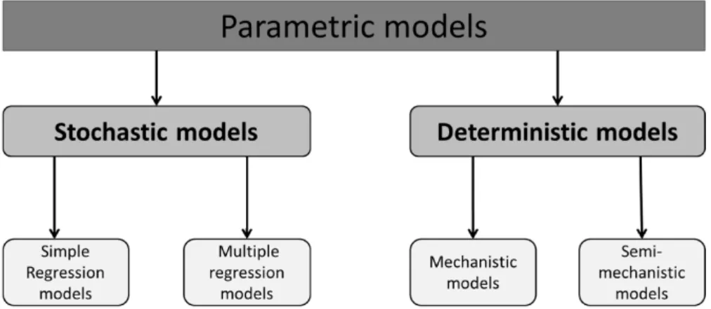
1.4.1. Parametric models ... 21
1.4.1.1. Simple regression models ... 22
1.4.1.2. Multiple regression models ... 23
1.4.1.3. Mechanistic models ... 24
1.5. Research focus ... 30
1.5.1. Research objectives ... 30
1.5.2. Dissertation outline ... 31
Chapter 2 - Evaluation of simple regression approaches to estimate the total biomass ... 33
2.1. Introduction ... 33
2.2. Materials and methods ... 34
2.2.1. Monitoring sites and plant biomass data ... 34
2.2.2. Seasonal NDVI integration ... 35
2.2.3. Seasonal NDVI maximum ... 35
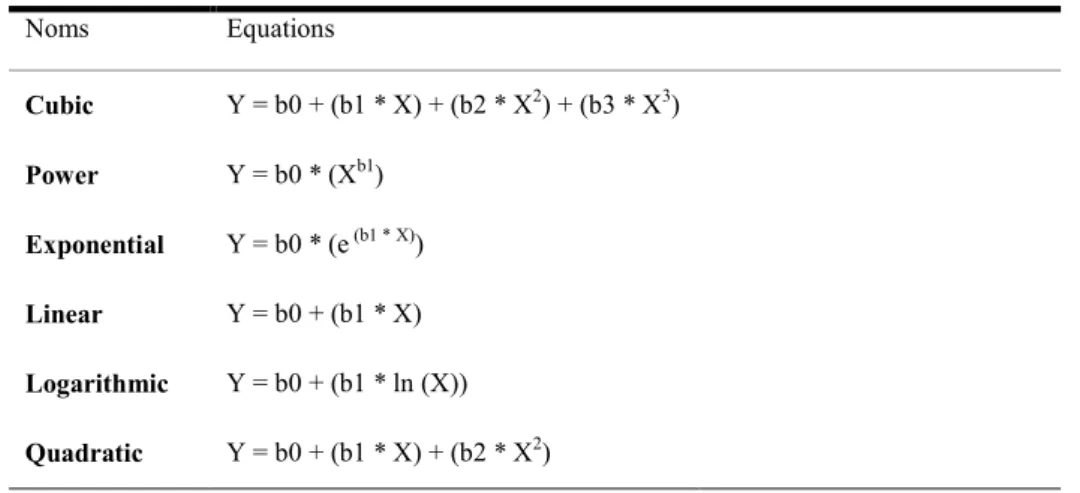
2.2.4. Statistical fitting functions ... 36
2.2.5. Assessment of model’s performance and coherence ... 37
2.3. Results ... 38
2.3.1. Statistical performance of fitted functions ... 38
2.3.2. Biophysical consistency of model estimations ... 40
2.3.3. Multiple year data-based estimates of total biomass ... 41
2.4. Discussion... 43
2.5. Conclusion ... 47
Chapter 3 - Total biomass estimation using multiple-linear regression models and phenological metrics from FAPAR time Series... 48
3.1. Introduction ... 48
3.2. Materials and methods ... 51
3.2.1. Study area and limit of studied ecoregions ... 51
3.2.2. Ground Biomass Data ... 53
3.2.3. Satellite Data ... 54
3.2.3.1. CSE biomass product ... 54
3.2.3.2. Phenological metrics from FAPAR time series ... 55
3.2.4. Modelling of the total plant biomass production ... 58
3.2.4.1. Reduction of explanatory variables and model development .. 58
3.3. Results ... 60
3.3.1. Relationship between total biomass and phenological variables 60 3.3.2. Importance of the explanatory variables in total biomass prediction ... 61
3.3.3. Selection and verification of the estimation models ... 62
3.3.4. Comparison with the NDVI-based CSE biomass product ... 64
3.3.5. Testing the multiple-predictor model for early warning ... 66
3.4. Discussion... 67
3.5. Conclusion ... 72
Chapter 4 - Herbaceous biomass estimation using machine learning models, agrometeorological data and metrics from FAPAR time Series ... 74
4.1. Introduction ... 74
4.2. Materials and methods ... 78
4.2.1. Study Area ... 78
4.2.2. Data and Processing... 79
4.2.2.1. Historical Field Herbaceous Yields ... 79
4.2.2.2. FAPAR Vegetation Dynamics and Calculated Metrics ... 80
4.2.2.3. Obtaining Agrometeorological Data ... 81
4.2.3. Methods ... 84
4.2.3.1. Explanatory Variable Selection for Herbaceous Mass Estimation ... 85
4.2.3.2. Rule-Based Regression Tree and Model Building ... 86
4.2.3.3. Model Verification, Error Analysis and Yield Anomaly Computation ... 87
4.3. Results ... 87
4.3.1. Variable Selection and Model Development ... 87
4.3.2. Spatio-Temporal Comparison of the Models’ Output ... 89
4.3.3. Season Onset/End Derived from FAPAR and Rainfall Data ... 92 4.3.4. Linkage between Start of the Growing/Rainy Season and Annual
4.4. Discussion... 95
4.4.1. Model Development and Output Comparison ... 95
4.4.2. Model Applicability and Uncertainties ... 96
4.4.3. Management Implications of Models Results ... 97
4.4.4. Comparison of FAPAR and Rainfall-Based Onset/End Metrics 98 4.4.5. Early Assessment of Herbaceous Yield from Onset Metrics ... 99
4.5. Conclusion ... 100
Chapter 5 - General conclusion and outlook ... 102
5.1. General conclusion ... 102
5.1.1. Total biomass estimation with simple regression models and NDVI variables ... 102
5.1.2. Total biomass estimation with multiple regression models and FAPAR metrics ... 103
5.1.3. Herbaceous forage estimation using FAPAR metrics and agrometeorological variables ... 104
5.2. Outlook ... 105
References ... 109
List of Figures
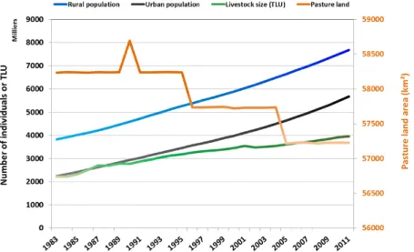
Figure 1.1 – Evolution of human and livestock population (in Tropical Livestock Unit or TLU) as well as grazing area from 1983 to 2011 in Senegal. Source: (FAOSTAT, 2016). ... 2 Figure 1.2 – Schematics of the general context of the natural resources use and
change in Senegalese rangelands ... 3 Figure 1.3 – Major Land cover classes of the Sahel provided by the GLC2000 map.
The Sahel limits are based on annual average precipitation (African Rainfall Climatology Version 2 1983–2013). ... 6 Figure 1.4 – Location of the study area and the ground control sites ... 7 Figure 1.5 – Inter-annual evolution of total biomass and rainfall anomalies (a), and
comparison of total biomass (b), herbaceous and woody leaf biomass contribution in global anomalies (c), and herbaceous and woody leaf biomass (d) with annual rainfall anomalies averaged in the dataset between 1999 and 2013 (ground biomass data are missing for 2004). Red arrows in (a) and (c) show the highest total biomass anomalies in the time series (i.e., years 2002 and 2010). Note that the relationship between rainfall and biomass is
strengthened when woody leaf and herbaceous biomass are added together. .. 12 Figure 1.6 – Distribution of all pixels of a scene into the red and near-infrared
bi-spectral space. Adapted from Silleos et al. (2006). ... 15 Figure 1.7 – Schematic classification of the main groups of parametric models. This scheme is not exhaustive and can be improved. ... 22 Figure 1.8 – STEP operation diagram representing the relationships between the
water balance and vegetation growth/senescence main modules. Adapted from Mougin et al. (1995). ... 26 Figure 2.1 – Statistical performance of the six models using the iNDVI ... 39 Figure 2.2 – Averaged statistical performance of the six models using the iNDVI
and NDVIpk predictors for the period 1999-2013. ... 39 Figure 2.3 – Estimates of total plant biomass within the 0.1-0.7 range of iNDVI and
NDVIpk, averaged from 1999 to 2013... 41 Figure 2.4 – Statistical difference of means of total biomass estimates made by
Exponential, Power and Linear models using the Wilcoxon signed rank test at 0.05 p-level. ... 43 Figure 2.5 – Example of total biomass predictions for the year 2002 with iNDVI and
NDVIpk. Negative predictions were masked out and correspond to the white pixels within the study area. ... 46 Figure 3.1 – Location of monitoring sites in the study area covering a range of
Sahelian ecosystems in Senegal. The isohyets are based on average rainfall estimates provided by FEWS Net between 1999 and 2013. ... 52 Figure 3.2 – Mean annual GEOV1 FAPAR time series for the four ecoregions in the study area. Phenological metrics are represented on the ECOsouth curve. For acronyms see Figure 1.4 and Table 2.3. ... 57
(VIP = 0.8) for the selection of key variables used for further model
development (ecoregions are shown in Figure 3.1). ... 62 Figure 3.4 – Relationships between observed and predicted total biomass by (a)
Model_SA, (b) Model_EW, (c) ecoregion models, and (d) CSE biomass product. Evaluation over the same validation dataset (n = 247 samples) from 2000 to 2013. The given statistics are the coefficient of determination (R²), the mean absolute error (MAE, kg·DM/ha), and the slope and offset of the linear regression equation. For color correspondence, see Figure 3.1. ... 65 Figure 3.5 – Temporal evolution of the estimated total biomass from CSE and
multiple predictor models with regard to observed total biomass, averaged from the monitored sites between 1999 and 2013. Ground data are missing for 2004. ... 66 Figure 3.6 – Total biomass estimates for (a) 2002 in deficit and (b) 2010 in surplus,
given by the early warning model (Model_EW). ... 67 Figure 3.7 – Scatterplots of anomalies of total biomass predicted by the early
warning model, with (a) observed total biomass and (b) rainfall from 1999 to 2013. ... 67 Figure 4.1 – Location of the monitoring sites and the main land cover classes (FAO
2009a). The isohyets are based on average rainfall estimates provided by FEWS Net between 2000 and 2015 (Xie and Arkin 1997). ... 78 Figure 4.2 – Seasonal FAPAR metrics considered in this study and shown for a
single pixel. The base value (BVAL) represents the averaged minimum values over the annual cycle (i.e., before and after the growing season). ... 81 Figure 4.3 – Overall crop coefficient curve for Senegal’s Sahelian rangelands during a growing season of 90 days. The growing period was divided into four phases: initial (i); vegetative (v); flowering (f); and ripening (r). SOSp indicates the mean date of the onset of the rainy season in the 2000-2015 period. Numbers in brackets indicate the total days of the phase. ... 84 Figure 4.4 – Workflow for the development of the rule-based piecewise regression
(i.e., Cubist) models for herbaceous yield estimation. ... 84 Figure 4.5 – Importance of the predictor variables for the three herbaceous yield
estimation models: (a) VI-model, (b) AGRO-model and (c) VIAGRO-model. Single variable importance initially given as the means of the percentage of use in model conditions and equations were then normalized to sum 100% for each model. ... 88 Figure 4.6 – Accuracy assessment of the developed Cubist models: relationship
between observed and predicted herbaceous yield for (a) the VI-model, (b) the AGRO-model and (c) the VIAGRO-model. ... 89 Figure 4.7 – Latitudinal variation of the herbaceous yield estimated by the (a)
VI-model, (b) AGRO-model and (c) VIAGRO-model during the 2000-2015 period. ... 90 Figure 4.8 – Coefficients of variation in annual herbaceous yield estimated by the
three models: (a) VI-model, (b) AGRO-model and (c) VIAGRO-model, according to the 2000-2015 average. ... 91
Figure 4.9 – Inter-annual variations in rainfall and estimated herbaceous yield over the whole study area from the (a) VI-model, (b) AGRO-model and (c) VIAGRO-model. Rainfall values were averaged from the 24 monitoring sites and the estimated herbaceous yield was averaged from all pixels covered by a given class. Colors and acronyms are explained in Figure 8.4 and Table 1.4. . 92 Figure 4.10 – Boxplots of the start and end of season metrics derived from FAPAR
(SOS and EOS) and rainfall data (SOSp and EOSp), averaged over the 2000-2015 period for each land cover class. ... 93 Figure 4.11 – Relationship between anomalies of herbaceous yield mass and onset of
(a) the growing season (SOS) and (b) the rainy season (SOSp) for the whole studied area, and (c) for each land cover class. Numbers on bars correspond to p-values. ... 94 Figure 5.1 – A1. Spatial distribution of percentage of missing data (MD) in yearly
FAPAR time series from 1999 to 2013 ... 136 Figure 5.2 – A2. Histograms of percentage of missing data in yearly FAPAR time
series from 1999 to 2013 ... 136 Figure 5.3 – A5. Averaged (a) herbaceous, (b) woody leaf and (c) total plant yield of the 24 sites used in this study and their corresponding standard deviation (error bar) for the 2000-2015 period. ... 138
List of Tables
Table 1.1 – The main medium and low spatial resolution satellites and their overall characteristics ... 13 Table 1.2 – Slope-based vegetation indices ... 16 Table 1.3 – Distance-based vegetation indices ... 17 Table 1.4 – Examples of machine learning algorithms usually applied in ecological
and environmental studies. ... 28 Table 2.1 – Basic equations of fitting functions ... 36 Table 2.2 – Statistical performance of the Exponential, Power and Linear models
calibrated with field sampling data of the period 1999-2013. The relative RMSE (RRMSE) in percentage was calculated using the averaged total biomass from all samples of the bootstrap dataset. ... 42 Table 3.1 – Description of ecoregions: vegetation type and main woody species,
annual rainfall (based on average values of RFE of FEWS Net data for the period 1999–2013), biomass, and woody cover based on ground measurements (1999–2013). The values for rainfall, woody leaf biomass, herbaceous
biomass, and woody cover correspond to the average from sites in each ecoregion. ... 53 Table 3.2 – Phenological metrics derived from the FAPAR time series (extracted
using TIMESAT software). ... 57 Table 3.3 – Criteria for the variable reduction, model selection, and validation. ... 59 Table 3.4 – Mean values, standard deviation (SD), and Pearson correlation statistics
of the phenological variables with total biomass collected in the 1999-2013 period (n = 263). For acronyms, see Table 3.2. ... 61 Table 3.5 – Calibration and bootstrap verification performances of multiple linear
regression models for total biomass estimation across the study area and per ecoregion. “n” is the size of the original sample used for calibration and “n_test” is the size of all bootstrap samples used for statistical calculations of verification. For other acronyms, see Tables 3.2 and 3.3. ... 63 Table 4.1 – General descriptions of land cover classes (FAO 2009c, d). Woody
cover values were obtained from the woody cover map provided by (Brandt et al. 2016) and correspond to the averaged values of pixels covered by classes. 79 Table 5.1 – A3. Description, unit and selection status after recursive feature
elimination and variable inflation control of 17 agrometeorological variables provided by the GeoWRSI water balance model and used in the study. The 10 underlined variables correspond to those used for model development. ... 137 Table 5.2 – A4. Mean signed difference (in dekads) between onset metrics
calculated from rainfall and FAPAR data across the agricultural and natural vegetation land cover classes in the study area. ... 137
1
Introduction
Chapitre 1 - Introduction
1.1. Research framework
1.1.1. General context and research justification
Livestock is the first renewable resource in Sahel (Dicko et al., 2006), and in particular West Africa. Livestock is dominated in this region by pastoral systems with large herds of cattle and small ruminants (RPCA, 2010). For this farming type, more than 90% of dry matter consumed by livestock comes from natural pastures (Carrière, 1996). Then, the rangelands form an indispensable component for meeting the needs of animal production in the West African Sahel. Also, they play an important ecological role, through soil fixing, carbon uptake and conservation of biodiversity. The grazing lands represent approximately 21% of the total area of Senegal (ISRA, 2003). They are largely dominated by natural pastures, and are found mainly in the eco-geographical zones of the Senegal River, the sylvo-pastoral zone (Ferlo), the eastern Senegal and the Upper Casamance.
As in the whole Sahel, the Senegalese farming systems have undergone the effects of drought and agricultural influence over grazing lands, since early 1970s. These actions drove firstly, to a significant reduction of the herbaceous cover, the dieback of woody plants (Wispelaere, 1980) and the change in species composition (Akpo, 1990), and secondly, to the abatement of natural rangelands available for pastoral livestock. The pasture lands varied from 58,232 km² in 1983 to 57,224 km² in 2011 with an area decrease about 2% (Figure 1.1). Following this dynamics, the rangelands quality also decreases in the long term, because the best lands are mostly reserved for agriculture (Carrière, 1996). The livestock size (i.e. Cattle, Sheep, Goats,
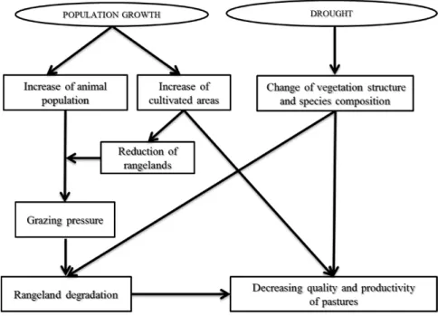
Horses, Asses and Camels) has largely increased over the past decades and therefore the fodder stock available at the end of the growing season is increasingly limited to meet the livestock feeding needs. This increase of animal population can be explained by the important role of livestock in the socioeconomic development of the Senegalese people that also highly increased in the same period. In Senegal, livestock provides about a third of the national agricultural wealth (Magrin, 2008; Cesaro et al., 2010). The animal production affects in particular a significant part of the rural population for which they provide food security, savings, labor force and field fertilization (ISRA, 2003). With the reduction of natural grazing lands, mostly generated by the expansion of croplands, and the decrease in pastures productivity due to drought effects, the increase of the livestock size leads to rangelands overload whose persistence can lead to their irreversible deterioration (CSE, 2010). Figure 1.2 shows a scheme of the overall context of the rangelands exploitation and their consequences.
Figure 1.1 – Evolution of human and livestock population (in Tropical Livestock Unit or TLU) as well as grazing area from 1983 to 2011 in Senegal.
Figure 1.2 – Schematics of the general context of the natural resources use and change in Senegalese rangelands
In this context, many studies have been conducted in the Sahel to establish methods for assessing the forage resources (Tucker et al., 1983; Tucker et al., 1985; Prince, 1991; Mougenot et al., 2000). Among these methods we can cite the one proposed by Tucker et al. (1983) and Tucker et al. (1985), including the temporal integration of the NDVI (Normalized Difference Vegetation Index) and the aboveground plant biomass produced during a growing season. This technique was revolutionary in 1980’s since it was the first time this new NDVI was related to field biomass data, through a simple linear regression. The overall approach has been operationally applied by the Centre de Suivi Ecologique (CSE) of Dakar (Diallo et al., 1991; Diouf and Lambin, 2001) (and also the Department of Livestock and Animal Industries of Niger) for evaluating the fodder biomass available in pasture lands at the end of the growing season. In Senegal, the sampling of herbaceous and woody foliar biomass is performed within ground sites distributed across the Senegalese pastoral domain that covers approximately fifteen administrative districts for an area of about 125,000 km². The ground biomass data collected each year have been typically used to calibrate by
regression the NDVI derived from the low resolution satellite imageries of the NOAA / AVHRR (from 1987 to 2002), SPOT / VEGETATION (from 2003 to 2013) and Proba-V (from 2014 to present). The output product is a map of the total plant biomass yield (kg.DM/ha) with 1 km resolution across the whole Senegal. This information carrier of the fodder biomass availability at the end of the growing season helps for assessing the balance between the amount of fodder biomass production and the livestock. It constitutes, therefore, a helpful guide tool for implementing the annual backup strategies and protection of pastoral flocks. It is also a useful tool for the identification of areas with very high dry matter production which could be a starting point of bushfires, and so to prevent against degradation of natural resources. However, there exists a significant time from the data collection and the publication of model results. Several studies also supported that the simple linear relationships developed annually depend highly on the ongoing growing season and the studied region (Cornet, 1984; Bégué, 2002). These facts of course, limit the operational capacity of the method specially to deal with the current needs of the early warning systems (EWS) on fodder biomass availability and of the public institutions in charge of environmental protection against bushfires. Despite these limitations, the approach has not changed over the last 30 years whereas the earth observation (EO) data have largely progressed. The EO data are more reliable with more cloud free images. With new methods implemented in various analysis tools (e.g. TIMESAT, SPIRITS, GeoWRSI etc.), seasonal profiles can be extracted from EO time-series and seasonal metrics computed accordingly either for vegetation products such as NDVI, the Fraction of Absorbed Photosynthetically Active Radiation (FAPAR), the Leaf Area Index (LAI) or for satellite based rainfall data. Making use of the new data and statistical methods which have emerged especially in the past 10 years, can allow improving the 1980’s approach to a newer state-of-the-art. Definitely, this enables to develop more suited tools for assessing more accurately the plant biomass production at the end of the growing season, and to make warnings as early as possible in the season applying specific
1.1.2. Main features of the studied region
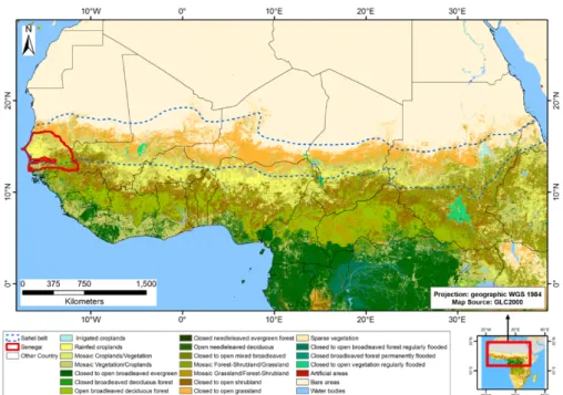
The Sahel name comes from two Arabic words, (i) Es-Sahel that means “shore” as “the shore of south Sahara” and (ii) S’hel ou Sahil meaning “plain” or “flatlands” (Tracol, 2004; Hiernaux and Le Houérou, 2006). Located between 12 °N and 20 °N latitudes, the Sahel is a biogeographic entity defined generally by its arid to semi-arid tropical climate (Hiernaux and Le Houérou, 2006), with an unimodal rainfall regime. The rainfall regime is mainly controlled by the monsoon from the Gulf of Guinea and the Sahara Harmattan. The Sahel is a transition zone between the arid to hyperarid Sahara areas in the north and the humid tropical areas of the south Sudan savanna (Brooks, 2004). It extends about 6000 km between the Atlantic Ocean (west) and the Red Sea (east) for a width between 400 and 600 km from north to south (Le Houerou, 1989). The Sahel belt passes over the Cape Verde, Mauritania, Senegal, Mali, Niger, Chad, Sudan and crosses the north of Burkina Faso, Nigeria and Cameroon, for a total area of 3 million km² (Tracol, 2004). Figure 1.3 shows the major land cover classes of the Sahel as proposed by the Global Land Cover 2000 (GLC2000) map (Bartholomé and Belward, 2005).
Part of the Sahel belt and member of the Comité inter-États de lutte contre la sécheresse au Sahel (CILSS), the Senegal covers an area of 196,722 km² and is located in the extreme west of Africa, between 12° 20' N and 16° 40' N latitude and 11° 20' W and 17° 30' W longitude. It is bounded by the Atlantic Ocean to the west, the Islamic Republic of Mauritania to the north and northeast, Mali to the east, Guinea Bissau and Guinea Conakry to the south. It also has a border with Gambia which draws an enclave of about 300 km long and 20 km width for an area of 10 300 km².
Figure 1.3 – Major Land cover classes of the Sahel provided by the GLC2000 map. The Sahel limits are based on annual average precipitation (African Rainfall
Climatology Version 2 1983–2013).
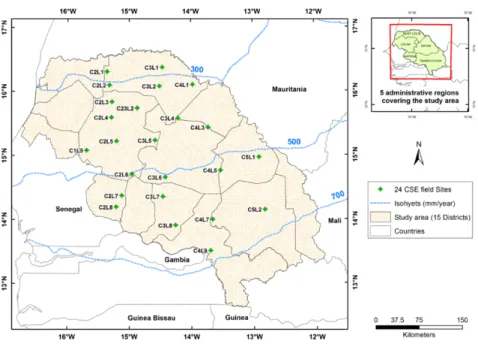
The study area covers 15 districts belonging to five administrative regions (i.e., Saint-Louis, Matam, Kaffrine, Louga and Tambacounda) in Senegal, with a total area of 125,000 km² (Figure 1.4). The area lies in the Sahelian and northern Sudano-Guinean zone of Senegal between 16.69°N and 12.63°N latitude and 16.74°W and 11.86°W longitude. It includes all natural grazing areas of the pastoral domain as defined by (Stancioff et al., 1986), as well as some croplands, including fallows. The mean annual precipitation varies between 200 and 980 mm from north to south, with reference to the FEWS Net rainfall estimates for the 2000-2015 period (Herman et al., 1997; Xie and Arkin, 1997). The rainy season, driven by the West African monsoon, is unimodal, occurring over 3-5 months between June and October. The studied area includes different ecoregions, with a prevalence of red-brown sandy soils, ferruginous tropical sandy soils, leptic, gley and vertic soils (Maignen, 1965; Tappan et al., 2004). Typical of the Sahel, the herbaceous vegetation is particularly dependent on the
intra-According to the Centre de Suivi Ecologique (CSE, 2013; CSE, 2014), the northern zone (<= 300 mm annual rainfall) is characterized by Poaceae such as Chloris prieurii, Aristida mutabilis and Dactyloctenium aegyptium, as well as legumes such as Alysicarpus ovalifolius and Zornia glochidiata, whereas in the central zone (between 300 and 500 mm) the characteristic species are Zornia glochidiata (Fabaceae) and Schoenfeldia gracilis, Pennisetum pedicellatum and Eragrostis tremula (all Poaceae). Towards the south, Andropogoneae species such as Andropogon pseudapricus and A. amplectans are the most common species. Other species, such as Spermacoce stachydea (Rubiaceae), Cassia obtusifolia (Fabaceae) and Fimbristylis exilis (Cyperaceae) occur irregularly, depending on the terrain morphology (e.g., depressions) and human and livestock influence.
Figure 1.4 – Location of the study area and the ground control sites
Note: All information provided about the study area has adapted from the publication (Diouf et al., 2016).
1.2. Monitoring sites and plant biomass data
The CSE established 36 ground control sites in 1987 for monitoring biomass at the end of the growing season in Senegalese pastoral areas. Among these sites, only 24 were monitored until now (see Figure 1.4) and used in this study. Sites are located in homogeneous vegetated zones of 3×3 km², making them ideal for comparison with moderate/coarse resolution remote sensing data. They are representative of the main geomorphological forms of sampled landscapes (Diallo et al., 1991). Sites were selected, indeed, based on a number of criteria as their accessibility, their uniformity in ecological conditions, their distance from the cropping areas and boreholes as well as their representativeness of the surrounding landscape. They are arranged in a grid (virtual) identified by its columns (C) and lines (L), hence their identification in Cx Ly, where x and y are numbers varying between 1 and 9 in relation to their position on the intersection of columns and lines into the grid (see sites name in Figure 1.4).
The in situ plant biomass data used in this research were obtained from the CSE database and covered the 1999–2015 periods, apart from 2004 when no data was collected. We have personally participated at data collection in 2013 and 2014 for the purposes of this thesis. The measurements were conducted annually at the end of the growing season (October), separately for the herbaceous and woody layers. The herbaceous and woody leaf biomass values were subsequently added together to provide an estimate of total plant biomass production, if any. The in situ data were not regularly collected, however, for all monitoring sites due to occasional lack of logistics or the early passage of bush fires before planned conductance of field campaigns.
1.2.1. Collection of herbaceous biomass
The collection technique used for the herbaceous layer was the stratified sampling line developed by the International Livestock Centre for Africa
line is allocated to one of four density/production strata, ranging from 0 to 3: 0 = bare soil; 1 = low production; 2 = medium production; and 3 = high production. Then, between 35 and 100 plots of one square meter are chosen randomly along the transect, taking account of the variability of different strata. The plant biomass in each plot is cut close to the ground and weighed with a precision scale. After three strata (low, medium, and high production) are re-sampled, only three samples of about 200 g of fresh material are taken back to the laboratory and dried in an oven (three samples for each stratum = nine samples for the site). They are dried for 48 h at 110 °C in order to obtain the dry matter.
The dry matter rate, obtained by dividing the dry weight of the sample by the green weight, is then integrated into an equation for calculating the herbaceous biomass production. The herbaceous dry matter production of the site is given by adding together the dry matter production of all three strata (low, medium, and high). For each stratum, the calculation equation is written as follows:
ℎ = × × × 10 (1)
where Ph is the herbaceous dry matter production (kg·DM.ha−1) in the stratum, fr is the relative frequency of the stratum along the transect, pm is the average green weight (g·m−2) measured in the field, ms is the dry matter rate, and 10 is a conversion factor for translating g·DM/m² into kg·DM/ha.
1.2.2. Collection of woody leaf biomass
The leaf biomass of trees and shrubs was sampled for each site in two steps, one repeated every 2 years and one annually. In the first step, every 2 years, four circular plots were delineated and centered at 200, 400, 600, and 800 meters of the 1000 m-long transect. The plot size depended on vegetation density and varied from 1 to 1/16 ha. The plots tended to be larger in the open land that characterizes the Sahelian area in the north of the study area and relatively smaller in the North Sudanian domain where the woody plant cover is denser. Within these plots, the parameters measured were
individual height, number of live trunks (some species, such as Guiera Senegalensis and Boscia Senegalensis, can have several trunks), plant cover, circumference at the base of the trunk(s), and phenological state (flowers, fruits, etc.). In the second step, the most representative species were sampled annually and, for each species type, 10 twigs were defoliated and fresh leaf biomass weighed. About 200 g of fresh leaves were dried and weighed in order to determine the leaf dry matter content. The primary foliage production of a given site reflected the total amount of leaf biomass produced for all trees and shrubs. Therefore, for each plant belonging to a given species, the primary foliage production (Pi) in kg was reached via an allometric relationship that integrates its circumference at the base. This relationship has been established for certain species of trees in the Sahel (Diallo et al., 1991; Diouf and Lambin, 2001) as a result of the work done by (Cissé, 1980) and (Hiernaux, 1980) in Mali. The expression is written as follows:
= × (2)
where a and b are two constants, depending on the species, and C is the base circumference of the trunk in cm.
The primary foliage production in kg of one species (Pe) within the four sampling plots of the site is obtained using the following formula where n represents the number of individual plants inventoried:
= (3)
The correction of this primary foliage production (including fruits, if any) (Cissé, 1980) into foliar production (Pf) (i.e., material that is available for the ongoing season and can be eaten by livestock as fodder) is done using the formula:
where Pve is the average weight of fresh foliar biomass (kg) of the 10 twigs, Mse is the dry matter rate in %, Ps0 is the average dry weight of foliar biomass (kg) of 10 twigs (reference value), and S is the total area of the four sampling plots in hectares.
Finally, the leaf biomass of one site was obtained by adding together the foliar production of all the inventoried woody species.
1.2.3. Plant biomass filtering
The ground measurements conducted by different people over 15 years were subject to uncertainty in sampling, measuring, and post-processing, which inevitably resulted in some unrealistic outliers. The post-processing of data (typing handwritten values into digital values) was never quality-checked, thus, in order to filter out obviously erroneous observations related to typos, etc., the datasets went through a two-step filtering: (1) first, the data were examined through an exploratory analysis of all observations using a boxplot with boundaries that were ±1.5 times the interquartile range and (2) since biomass production in Sahel is highly dependent on rainfall (Figure 1.10), a second filtering of biomass estimates was conducted with outliers identified in the first step to remove unrealistic values that showed no relation to the rainfall estimates obtained from FEWS Net imagery (Xie and Arkin, 1997). This rainfall data has a resolution of 8 km and is thus able to capture the heterogeneous pattern of the study area. Only those observations for which the difference between the anomalies of plant biomass and anomalies of annual rainfall was less than 65% were selected. This threshold value was determined by referring to the total biomass anomalies explained by the linear regression with rainfall anomalies (Figure 1.5b). The filtering removed 33 observations in the 1999–2013 periods, leaving 263 observations in the dataset for further analysis. This dataset was used into Chapter 2, and 3 while for Chapter 4, 34 observations from the years 2014 and 2015 were added to the dataset after they have been checked with same procedure described above.
Figure 1.5 – Inter-annual evolution of total biomass and rainfall anomalies (a), and comparison of total biomass (b), herbaceous and woody leaf biomass contribution in global anomalies (c), and herbaceous and woody leaf biomass (d) with annual rainfall anomalies averaged in the dataset between 1999 and 2013 (ground biomass data are missing for 2004). Red arrows in (a) and (c) show the highest total biomass anomalies in the time series (i.e., years 2002 and 2010). Note that the relationship between rainfall and biomass is strengthened when woody leaf and herbaceous biomass are added together.
Note: All information provided in this Section 1.2.2 have been adapted from the paper (Diouf et al., 2015).
1.3. Remote sensing data
After the launch of the first Landsat satellite in 1972, many studies had demonstrated the advantages of using satellite remote sensing data for vegetation monitoring, with indices using the reflectance recorded by the satellite sensors. That is why the United Nations Conference on the Human Environment, held in Stockholm in 1972, suggested use of the remote sensing as a tool of "direct global monitoring" (Grainger, 2013). For monitoring the vegetation cover across the world, various satellite from medium to low spatial resolutions were launched and several indices and biophysical products developed for many application. The overall characteristics of the most used satellites in the past 40 years are shown in
Table 1.1 – The main medium and low spatial resolution satellites and their overall characteristics
Satellite NOAA SPOT TERRA/AQUA MSG ENVISAT METOP PROBA SENTINEL3
Sensor AVHRR VGT MODIS SEVERI MERIS AVHRR V OLCI
Frequency daily daily 1/2 days 15mn 3/5 days daily daily 1/2 days
Spatial resolution 1.1km 1km 250/500m 3km 300/1000m 1km 300/1000m 300m Swath width 2800km 2,200km 2300km hemisphere 1150km 2500km 2500km 1270Km
Wavelength (nm) Blue 430-470 437.5 - 447.5 Red 580-680 610-680 620 - 670 560-710 677.5 - 685.0 580-680 NIR 725-1000 780-890 841 - 876 740-880 855 - 875 725-1000 Service start 1979 1998 1999 2002 2003 2007 2013 2016
1.3.1. Vegetation indices products
There exist a large variety of quantitative indices of vegetation conditions using remote sensing instruments. These vegetation indices (VIs) measure the green vegetation that has the particularity through the chlorophyll to absorb solar energy for use in the photosynthesis process. The green vegetation has a variable spectral signature related to the chlorophyll activity in plants. In favorable conditions (healthy canopies), the chlorophyll in green vegetation absorbs red portion (Red) of the electromagnetic spectrum, while the near-infrared portion (NIR) is strongly scattered by the spongy structure of the mesophyll in leaves, due to the presence of numerous intercellular spaces. In contrast when conditions are unfavorable, for example in situations of water deficit, the NIR reflectance is low, while the return of Red (poorly absorbed) to the sensor is higher. It is this contrast between Red and NIR reflectance by canopies of green vegetation that has been considered to develop the large set of existing VIs nowadays. The VIs can be classified into two groups after (Baret and Guyot, 1991; Jackson and Huete, 1991): (1) ratios (or slope-based) and (2) linear combinations (or distance-based) VIs. Figure 1.6 shows a schematic distribution of pixels within a bi-dimensional plot (scattergram) of Red against NIR reflectance of a given scene, and allows easy distinction of these two groups.
Figure 1.6 – Distribution of all pixels of a scene into the red and near-infrared bi-spectral space. Adapted from Silleos et al. (2006).
The slope-based VIs are simple ratio, or the ratio of sums, differences or products of the Red and NIR spectral bands (Jackson and Huete, 1991; Pettorelli, 2013). These VIs focus on the contrast between the spectral response patterns of green vegetation in the red and near-infrared portions of the electromagnetic spectrum and their values indicate both the state and abundance of green vegetation cover and plant biomass (Silleos et al., 2006). The position of each point in the 2-dimensional Red-NIR space is geometrically equivalent to the slope of the line connecting the origin of reference and this particular point on the scattergram (Mróz and Sobieraj, 2004). Table 1.2 shows the main slope-based VIs used in the literature.
Table 1.2 – Slope-based vegetation indices
Name Formula Author
Ratio Vegetation Index
(standard) = Birth and McVey (1968)
Normalized Difference Vegetation Index = − + Rouse et al. (1974) Soil-Adjusted Vegetation Index = (1 + ) Huete (1988) Transformed Vegetation Index = − + + 0.5 Deering et al. (1975)
Ratio Vegetation Index
(inverse) =
Richardson and Wiegand (1977)
Enhanced Vegetation Index
= ∗ −
+ − + Liu and Huete (1995)
Where NIR = near-infrared, R = red, B = blue, L = soil adjustment factor, C1 and C2 = constants and G = a gain factor.
The distance-based VIs are functionally different to the slope-based ones and are computed from linear combinations of the Red and NIR bands. These VIs are calculated by taking into account the difference of any pixel’s reflectance from the reflectance of bare soil (Baret and Guyot, 1991; Silleos et al., 2006). This requires establishing the “soil line” that corresponds to the linear regression line of the NIR band against the Red band for a sample of bare soil pixels. Then it enables to remove the effect of soil brightness in cases where vegetation is sparse and pixels are supposed to be contaminated by the soil background. Pixels located near the soil line are assumed to represent the soil, while those far away are assumed to represent vegetation. The distance-based VIs require the slope and intercept of the soil line as inputs for their calculation as well. Table 1.3 shows examples of distance-based VIs frequently cited in the literature.
Table 1.3 – Distance-based vegetation indices
Name Formula Author
Perpendicular Vegetation Index 1
PVI =(aNIR − R) + b √a + 1
Perry Jr and
Lautenschlager (1984) Difference Vegetation Index
DVI = aNIR − R Richardson and Wiegand
(1977) Weighted Difference Vegetation
Index WDVI = NIR − aR Clevers (1988)
Transformed Soil-Adjusted
Vegetation Index 1 TSAVI =
a(NIR − aR − b)
R + aNIR − ab (Baret et al., 1989) Modified Soil-Adjusted Vegetation
Indices 1 MSAVI =
(1 + L) Qi et al. (1994)
Where NIR = near-infrared, R = red, a and b are slope and intercept of the soil line respectively, L = 1- 2*a*NDVI*WDVI (Weighted near-infrared-red Difference Vegetation Index)
Among all VIs, the NDVI remain the most commonly used in the Sahel for the quantification and temporal monitoring of the vegetation covers (Bénié et al., 2005). Indeed, it gives a quantitative measure that only yields relative estimates of vegetation amounts, but it can be used to better reflect the actual changes in primary production, as well as for quantification of its absolute value (Seaquist et al., 2003). NDVI time series were used in several studies to depict information on the spatial distribution of bioclimatic zones (Jönsson and Eklundh, 2004) and also on their cover change/trend over time (Anyamba and Tucker, 2005; Wei et al., 2012; Brandt et al., 2014).
1.3.2. Vegetation biophysical products
The Fraction of Photosynthetically Active Radiation absorbed by vegetation (FAPAR) and the Leaf Area Index (LAI) are important biophysical variables for quantifying interactions between the vegetation surface and the atmosphere (Myneni et al., 2002; Tian et al., 2004; Demarty et al., 2007; Baret et al., 2013). LAI and FAPAR represent two biophysical complementary ways of describing the earth's vegetated surfaces (Fensholt et al., 2004) and they play a key role in several surface processes, including
photosynthesis, transpiration rates, rainfall interception and gas exchange. For this raison, they have been identified by the GCOS (2006) to be essential terrestrial climate variables in the context of global change studies.
Defined as half of the total intercepting area per unit ground surface area (m² leaf area per m² ground area) (Chen and Black, 1992), the LAI characterizes the functioning surface area of a vegetation canopy (Myneni et al., 2002) and it quantifies the thickness of the green leaf area of terrestrial vegetation (Fensholt et al., 2004). Satellite remote sensing enables retrieval of LAI with algorithms based on the physics of radiative transfer (Hanes, 2014). FAPAR is defined as the fraction of photosynthetically active radiation (400–700nm) absorbed by the vegetation canopy and expresses, thus, a canopy's energy absorption capacity (Fensholt et al., 2004; Fan et al., 2014; Hanes, 2014). In order to avoid the local-specific disadvantage of empirical methods (i.e., statistical) which use spectral vegetation indices (e.g., NDVI) or LAI to calculate the FAPAR, physical inversion methods are commonly used nowadays based on radiative transfer models (Knyazikhin et al., 1998; Myneni et al., 2002; Baret et al., 2007; Gobron et al., 2007; Fan et al., 2014; Li et al., 2015). These latter models which describe the transfer of solar radiation in vegetation canopies are generally based on the energy conservation law (transmittance, reflectance and absorptance of the canopy) and retrieve the FAPAR products using satellite remote sensing observations (e.g., canopy spectral and directional characteristics) as constraints (Knyazikhin et al., 2004; GCOS, 2006). Plant biomass production is closely related to light interception (van Wijk and Williams, 2005), which is determined by FAPAR and LAI. These products, therefore, were used as key variables in many models of net primary production (NPP) to calculate the surface ecosystems productivity (Potter et al., 1993; Field et al., 1995; Running et al., 1999). Both FAPAR and LAI products are globally available now, through remotely sensed imagery, at different spatial resolutions (250– 1000m) and temporal frequency (10–30days).
1.3.3. Rainfall estimates dataset
The number of rain gauges throughout Africa is small and unevenly distributed, and the gauge network is deteriorating (Dinku et al., 2007), explaining accordingly the difficulty to access on field rainfall data. Satellite rainfall estimates constitutes valuable products to ensure continuity of environmental studies in these areas. Several rainfall products have been elaborated and are generally freely available in various temporal and spatial levels. The product used in this research called FEWS Net RFE is produced by NOAA’s Climate Prediction Center (CPC) specifically for United States Agency for International Development (USAID) Famine Early Warning Systems (FEWS) to assist in drought monitoring activities over Africa (Dinku et al., 2007). The first version (RFE v1.0) was produced from 1995 to 2000 (Herman et al., 1997) and was replaced from 2001 onwards by the RFE v2.0. This latest version is a blended product based on cold cloud duration (CCD) derived from Meteosat thermal infrared (TIR), estimates from the Special Sensor Microwave Imager (SSM/I) and the Advanced Microwave Sounding Unit (AMSU), and daily station rainfall data (Toté et al., 2015). The main difference between these two versions is that RFE v2.0 uses passive microwave (PM) estimates while RFE v1.0 includes a procedure to estimate warm orographic rain (Dinku et al., 2007). Particularly, RFE v2.0 product was shown to be in good agreement with ground rainfall data (Jobard et al., 2011). Linear regression between annual FEWS Net RFE and field data collected in the period 1996-2012 for Linguere, Podor, Matam and Tambacounda gauge stations gave a coefficient of determination of 0.788. The data are available over Africa and freely accessible at (http://earlywarning.usgs.gov/fews/datadownloads) in dekadal time step and 8 km spatial sampling grid.