arXiv:1112.5145v2 [astro-ph.EP] 22 Jan 2013
Thermal emission at 3.6–8 µm from WASP-19b: a hot
Jupiter without a stratosphere orbiting an active star
D. R. Anderson,
1⋆A. M. S. Smith,
1N. Madhusudhan,
2P. J. Wheatley,
3A. Collier Cameron,
4C. Hellier,
1C. Campo,
5M. Gillon,
6J. Harrington,
5P. F. L. Maxted,
1D. Pollacco,
7D. Queloz,
8B. Smalley,
1A. H. M. J. Triaud
8and R. G. West
91Astrophysics Group, Keele University, Staffordshire ST5 5BG, UK
2Department of Astrophysical Sciences, Princeton University Princeton, NJ 08544, USA 3Department of Physics, University of Warwick, Coventry, CV4 7AL, UK
4School of Physics and Astronomy, University of St. Andrews, North Haugh, Fife, KY16 9SS, UK
5Planetary Sciences Group, Department of Physics, University of Central Florida, Orlando, FL 32816-2385, USA 6Institut d’Astrophysique et de G´eophysique, Universit´e de Li`ege, All´ee du 6 Aoˆut, 17, Bat. B5C, Li`ege 1, Belgium
7Astrophysics Research Centre, School of Mathematics & Physics, Queen’s University, University Road, Belfast, BT7 1NN, UK 8Observatoire de Gen`eve, Universit´e de Gen`eve, 51 Chemin des Maillettes, 1290 Sauverny, Switzerland
9Department of Physics and Astronomy, University of Leicester, Leicester, LE1 7RH, UK
Accepted 2013 January 22. Received 2013 January 21; in original form 2011 December 21
ABSTRACT
We report detection of thermal emission from the exoplanet WASP-19b at 3.6, 4.5, 5.8 and 8.0 µm. We used the InfraRed Array Camera on the Spitzer Space Telescope to observe two occultations of WASP-19b by its host star. We combine our new detections with previous measurements of WASP-19b’s emission at 1.6 and 2.09 µm to construct a spectral energy distribution of the planet’s dayside atmosphere. By comparing this with model-atmosphere spectra, we find that the dayside atmosphere of WASP-19b lacks a strong temperature inversion. As WASP-19 is an active star (log R′
HK= −4.50±
0.03), this finding supports the hypothesis of Knutson, Howard & Isaacson (2010) that inversions are suppressed in hot Jupiters orbiting active stars. The available data are unable to differentiate between a carbon-rich and an oxygen-rich atmosphere. Key words: methods: data analysis – techniques: photometric – occultations – plan-ets and satellites: atmospheres – planplan-ets and satellites: individual: WASP-19b – stars: individual: WASP-19.
1 INTRODUCTION
By observing the occultation of an exoplanet by its host star, we can measure the emergent flux from the planet’s day-side atmosphere. Such measurements are challenging due to the low planet-to-star flux ratio (for the best cases, typ-ically a few tenths of one per cent in the near infrared) and sources of noise both instrumental and stellar in origin (e.g.: Knutson et al. 2008; Smith et al. 2011). To date, most such measurements (including the first, Charbonneau et al. 2005; Deming et al. 2005) have been made with the Spitzer Space Telescope, though ground-based facilities are now an essential complement (e.g.: de Mooij & Snellen 2009; Sing & L´opez-Morales 2009).
With a single occultation we can measure the cor-responding brightness temperature and determine the ec-centricity of the planet’s orbit (e.g. Charbonneau et al. 2005), which is necessary for the accurate determination of the stellar and planetary radii in transiting systems (Anderson et al. 2012) and is important for studies of the formation and tidal inflation of short-period, giant plan-ets (e.g.: Nagasawa & Ida 2011; Ibgui, Burrows & Spiegel 2010).
With photometric measurements at various wave-lengths, we can construct a spectral energy distribution of the planet’s dayside atmosphere. From this we can infer properties such as the planetary albedo, the dayside en-ergy budget and the efficiency of dayside-to-nightside enen-ergy redistribution (e.g. Barman, Hauschildt & Allard 2005). As the atmospheric depth probed depends on the molecular
opacity in the observation band, a spectrum can describe an atmosphere’s vertical temperature structure. The obser-vation that some planet atmospheres exhibit strong tem-perature inversions, or stratospheres, and others do not (see Knutson, Howard & Isaacson 2010, for a summary) led to a suggestion that inversions are present in atmo-spheres hot enough to maintain high-opacity absorbers in the gas phase in the upper atmosphere (e.g. Fortney et al. 2008). However, this was challenged by recent contrary re-sults (Machalek et al. 2008; Fressin et al. 2010) and theory (e.g. Spiegel, Silverio & Burrows 2009). As an alternative, Knutson, Howard & Isaacson (2010) suggested that those planets orbiting chromospherically active stars lack inver-sions because the associated high UV flux destroys the high-opacity, high-altitude compounds that would otherwise in-duce inversions. This hypothesis is based on a small sample and further measurements across a wider parameter space are vital to test it. Specifically, there is a paucity of mea-surements for planets orbiting active stars. We suggest com-position could be a key factor, with low-metallicity planets lacking high concentrations of the high-opacity absorbers, such as TiO and sulphur, thought to be responsible for in-versions (e.g. Fortney et al. 2008; Zahnle et al. 2009).
As the spectral coverage increases, so too does the information about an atmosphere that we can discern. Madhusudhan et al. (2011a) used seven measurements of the emission of WASP-12b (Croll et al. 2011; Campo et al. 2011) to show that the dayside atmosphere is the first known to be carbon-dominated. Thus we are entering an era in which we can make statistically-sound inferences about the composition of exoplanet atmospheres. Further, Madhusudhan et al. (2011a) demonstrated that the planet lacks a prominent thermal inversion and has very inefficient day-night energy circulation.
In this paper, we present Spitzer measurements of WASP-19b’s dayside thermal emission at 3.6, 4.5, 5.8 and 8.0 µm. Discovered by the Wide Angle Search for Planets (Pollacco et al. 2006; Hebb et al. 2010), the shortest-period hot Jupiter, WASP-19b, is a 1.17-MJup planet in a
near-circular, 19-hr orbit around a G8V star. Hellier et al. (2011) showed the planet’s orbital axis to be aligned with the spin axis of its host star. The planet’s thermal emission was pre-viously measured at 1.6 and 2.09 µm (Anderson et al. 2010; Gibson et al. 2010), thus we bring the measurement tally to six bands. We use all six thermal emission measurements to characterise the planet’s atmosphere and refine the sys-tem parameters by combining these data with pre-existing photometry of the transit and radial-velocity data.
2 NEW OBSERVATIONS
We observed two occultations of the planet WASP-19b by its host star WASP-19 (2MASS 15595095−2803422, Ks =
10.22) with Spitzer (Werner et al. 2004) during UT 2009 January 29 and UT 2009 March 22. On each date, we em-ployed the Infrared Array Camera (IRAC, Fazio et al. 2004) in full array mode (256 × 256 pixels, 1.2 ′′ pix−1). During
the first occultation, we measured the WASP-19 system si-multaneously in the 4.5- and 8.0-µm channels (respectively, channels 2 and 4) for a duration of 3.2 h. We measured the second occultation simultaneously in the 3.6 and 5.8 µm
channels (respectively, channels 1 and 3) for a duration of 3.0 h.
Prior to the first occultation, we used the emission neb-ula NGC 7538 in Cepheus to ‘pre-flash’ the target position on the detector arrays for 0.5 hr. This was intended to reduce or remove the known illumination-history dependence of the gain response of the 8.0-µm detector (e.g. Knutson et al. 2008, and references therein). The 5.8-µm detector is known to suffer a similar issue, but pre-flashing this array was not permitted due to the detrimental effect it is known to have on the array. Instead, we attempted to stabilize the array by observing the target for an extra hour prior to the oc-cultation. As this ‘pre-stare’ was performed as a separate observation request to the occultation observation, the tar-get was reacquired between the two. As such, the pre-stare observation must be treated as a separate dataset with its own systematics and so are of little use in determining the occultation depth.
Using an effective integration time of 10.4 s, we ob-tained 876 and 840 images, respectively, for the first and second occultations. In each dataset, we see a small, peri-odic, pointing wobble (P ≈ 1 hr), thought to be caused by the thermal cycling of an on-board battery heater1. There
is also a very small drift of the target position over the span of each dataset.
We used the images calibrated by the standard Spitzer pipeline (version S18.7.0) and delivered to the community as Basic Calibrated Data (BCD). Our method is essentially the same as we presented in Anderson et al. (2011b), to which we refer the reader for further information. For each im-age we converted flux from MJy sr−1 to electrons and then
used iraf to perform aperture photometry for WASP-19, using circular apertures with a range of radii: 1.5–6 pixels for the 3.6 µm and 4.5 µm data and 1–5 pixels for the 5.8 µm and 8.0 µm data. The apertures were centred by fit-ting a Gaussian profile on the target. The sky background was measured in an annulus extending from 8 to 12 pixels from the aperture centre, and was subtracted from the flux measured within the on-source apertures. We estimated the photometric uncertainty as the quadrature addition of the uncertainty in the sky background (estimated as the stan-dard deviation of the flux in the sky annulus) in the on-source aperture, the read-out noise, and the Poisson noise of the total background-subtracted counts within the on-source aperture. We calculated the mid-exposure times in the HJD (UTC) time system from the MHJD OBS header values, which are the start times of the DCEs (Data Col-lective Events), by adding half of a DCE duration (FRAM-TIME).
The choice of aperture radius for each dataset was a compromise between maximising the signal-to-noise of the measurements and, from fits to all available data (see Section 3), minimising the residual scatter of the lightcurve. Each consideration suggested very similar optimal apeture radii and we adopted 2.7 pix for the 3.6- and 4.5-µm data and 2.5 pix for the 5.8- and 8.0-µm data. For each dataset we found that the variation in the fitted occultation depth (see Section 3) was much smaller than 1 σ over a wide range of aperture radii.
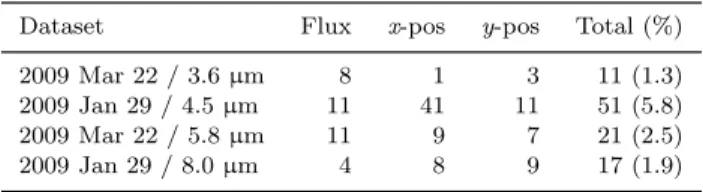
Table 1.Number of points rejected per dataset per criterion
Dataset Flux x-pos y-pos Total (%)
2009 Mar 22 / 3.6 µm 8 1 3 11 (1.3)
2009 Jan 29 / 4.5 µm 11 41 11 51 (5.8)
2009 Mar 22 / 5.8 µm 11 9 7 21 (2.5)
2009 Jan 29 / 8.0 µm 4 8 9 17 (1.9)
Some groups choose to reject a portion of data at the beginning of each observation, citing as justification either the settling of the spacecraft (not seen in our data) or an improvement in the fit; we found no reason to do this. We rejected any flux measurement that was discrepant with the median of its 20 neighbors (a window width of 4.4 min) by more than four times its theoretical error bar. We also per-formed a rejection on target position. For each image and for the x and y detector coordinates separately, we com-puted the difference between the fitted target position and the median of its 20 neighbors. For each dataset, we then calculated the standard deviation, σ, of these median differ-encesand rejected any points discrepant by more than 4 σ. The numbers of points rejected on flux and target position for each dataset are displayed in Table 1. According to the IRAC handbook, each IRAC array receives approximately 1.5 solar-proton and cosmic-ray hits per second, with ∼2 pixels per hit affected in channels 1 and 2, and ∼6 pixels per hit affected in channels 3 and 4, and the cosmic ray flux varies randomly by up to a factor of a few over time scales of minutes. Thus, the average probability per exposure that pixels within the stellar aperture will be affected by a cos-mic ray hit is 1.3 per cent for channels 1 and 2 and 3.2 per cent for channels 3 and 4, which is in good agreement with the portion of frames that we rejected. These probabilities are likely to be underestimates as we calculated them using partial pixels and neglecting the effect of hits within the sky annuli. For an unknown reason, a greater portion of channel 2 images were rejected due to jumps of the target position, particularly in the x direction. The post-rejection data are displayed raw and binned in the first and second panels re-spectively of Figure 1.
3 DATA ANALYSIS 3.1 Data and model
We performed a global determination of the system pa-rameters incorporating: our new Spitzer occultation pho-tometry; the HAWK-I H-band and 2.09-µm occultation lightcurves obtained, respectively, by Anderson et al. (2010) and Gibson et al. (2010); the 34 CORALIE radial-velocity (RV) measurements listed in Hebb et al. (2010); the 36 HARPS RVs, obtained through a transit, and the 3 CORALIE RVs given in Hellier et al. (2011); the LCOGT FTS z-band transit lightcurve from Hebb et al. (2010); and the ESO NTT r-band transit lightcurve presented in Hellier et al. (2011). We did not include the three seasons of WASP survey photometry presented in Hebb et al. (2010). Rather, we placed a Bayesian Gaussian prior on the epoch of mid-transit, Tc, using the epoch given in Hellier et al.
(2011): Tc= 2455168.96801 ± 0.00009 HJD. Thus our
anal-yses completed quicker and the shape of the transit was determined using only the high-S/N photometry. This can be preferable as photometry from surveys such as WASP is prone to dilution and, depending on which detrending al-gorithm is used, the transit depth can be suppressed. We decorrelated each transit lightcurve with a linear function of time. The HAWK-I H-band data were partitioned and detrended as in Anderson et al. (2010) and the HAWK-I 2.09-µm lightcurve was decorrlelated with a linear function of time as in Gibson et al. (2010). These data were used as input into an adaptive Markov-chain Monte Carlo (MCMC) algorithm (Collier Cameron et al. 2007; Pollacco et al. 2008; Enoch et al. 2010); see Anderson et al. (2011a) for a descrip-tion of the current version of our code. Such an analysis, in-corporating all available data, is necessary to take account of the cross-dependancy of system parameters and to make a reliable assessment of their uncertainties. We partitioned the RV data by spectrograph so as to allow for an instru-mental offset and for a potential specific stellar activity level during the short-baseline HARPS observations.
The MCMC proposal parameters we used are: Tc,
P , (Rpl/R∗)2, T14, b, K1, Teff, [Fe/H], √e cos ω, √e sin ω,
√
v sin i cos λ, √v sin i sin λ, ∆F1.6, ∆F2.09, ∆F3.6, ∆F4.5,
∆F5.8, ∆F8.0 and toff. See Section 3.2 for a definition of
toff and Table 3 for definitions of the other parameters. At
each step in the MCMC procedure, each proposal parame-ter is perturbed from its previous value by a small, random amount. From the proposal parameters, model light and RV curves are generated and χ2 is calculated from their
com-parison with the data. A step is accepted if χ2 (our merit function) is lower than for the previous step, and a step with higher χ2 is accepted with probability exp(−∆χ2/2). In this way, the parameter space around the optimum so-lution is thoroughly explored. The value and uncertainty for each parameter are respectively taken as the median and central 68.3 per cent confidence interval of the param-eter’s marginalised posterior probability distribution (e.g. Ford 2006).
3.2 Spitzer data
IRAC uses an InSb detector to observe at 3.6 and 4.5 µm, and the measured flux exhibits a strong correlation with the position of the target star on the array. This effect is due to the inhomogeneous intra-pixel sensitivity of the detector and is well-documented (e.g. Knutson et al. 2008, and references therein). Following Charbonneau et al. (2008) we modelled this effect as a quadratic function of the sub-pixel position of the PSF centre, with the addition of a cross-term to permit rotation (D´esert et al. 2009) and a linear term in time:
df = a0+axdx+aydy+axydxdy+axxdx2+ayydy2+atdt (1)
where df = f − ˆf is the stellar flux relative to its weighted mean, dx = x − ˆx and dy = y − ˆy are the coordinates of the PSF centre relative to their weighted means, dt is the time elapsed since the first observation, and a0, ax, ay, axy, axx,
ayyand atare coefficients.
IRAC uses a SiAs detector to observe at 5.8 and 8.0 µm, and its response is thought to be homogeneous, though another systematic affects the photometry. This effect is
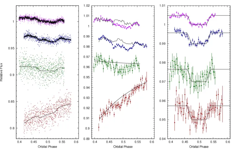
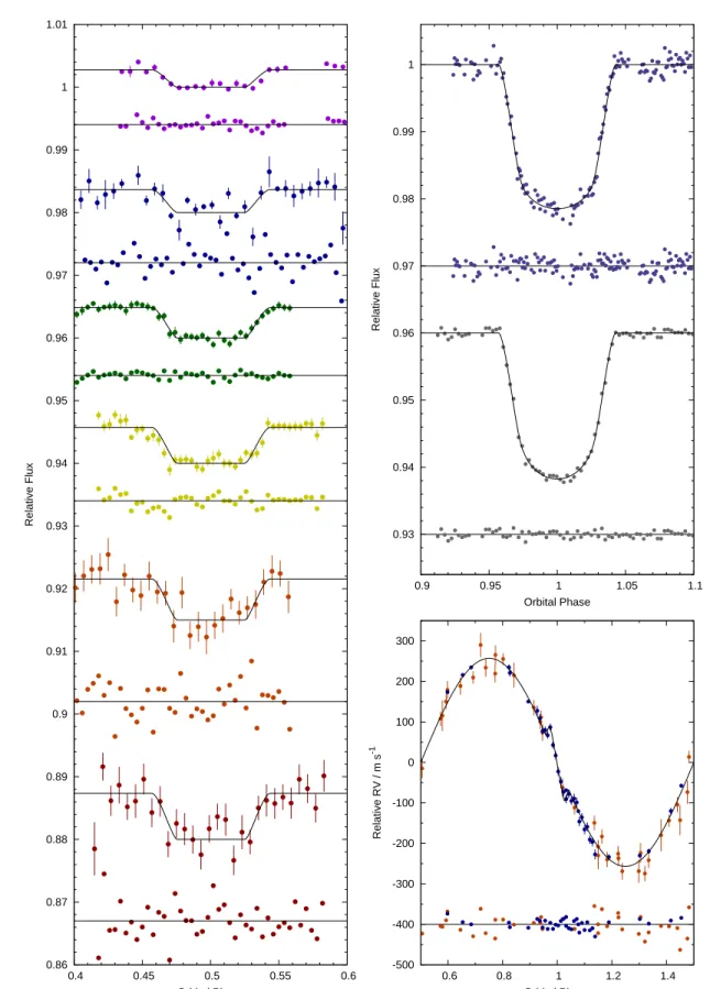
Figure 1. In each of the above three plots, from top to bottom, the data were taken at 3.6, 4.5, 5.8 and 8.0 µm. Relative flux offsets were applied to datasets for clarity. Left: Raw Spitzer data with the best-fitting trend and occultation models superimposed. Middle: The same data binned in phase (∆φ = 0.003 ∼ 3.4 min) with the best-fitting trend models superimposed. Right: The binned data after dividing by the best-fitting trend models, and with the best-fitting occultation models superimposed. The error bar on each binned measurement in the panels in the middle and on the right is the standard deviation of the points within the bin.
Table 2.Trend model parameters and coefficients
3.6 µm 4.5 µm 5.8 µm 8.0 µm ˆ f 151194.55 80580.23 12693.57 18991.68 ˆ x 31.93 24.50 25.99 25.44 ˆ y 24.91 25.98 25.16 23.63 a0 −24 ± 16 89.7 ± 5.0 −95.2+26−22 1569 +142 −116 ax 6566 ± 75 −433 ± 36 — — ay 9278 ± 49 4062 ± 32 — — axy 6040 ± 3280 −7860 ± 4150 — — axx −6330 ± 1230 23000 ± 880 — — ayy −22500 ± 1980 30360 ± 3810 — — at 1050 ± 270 −2203 ± 57 — — a1 — — −52+21−11 800 +110 −86 a2 — — −5.9+4.1−1.4 78+18−13 toff/min — — 10.6+11.4−8.1 15.3+10.1−7.4
known as the ‘ramp’ because it causes the gain to in-crease asymptotically over time for every pixel, with an amplitude depending on a pixel’s illumination history (e.g. Knutson et al. 2008, and references therein). Again follow-ing Charbonneau et al. (2008), we modelled this ramp as a quadratic function of ln(dt):
df = a0+ a1ln(dt + toff) + a2(ln(dt + toff)) 2
(2)
where toff is a proposal parameter restricted to positive
val-ues. To prevent toff from drifting to values greater than an
hour or so, we place on it a Gaussian prior by adding a Bayesian penalty to our merit function (χ2):
BPtoff = t
2 off/σ
2
toff (3)
where σtoff = 15 min.
A steep ramp is evident in the 8.0-µm lightcurve (Fig-ure 1, middle panel). Due to the large distance on the sky between the target and the pre-flash source, there was an 11-minute gap between the end of the pre-flash observations and the start of the target observations. It may be that the detector traps de-populated during this time, giving rise to the observed ramp that is more typical of observations with-out pre-flash.
In addition to Equation 2, we tried trend functions with a variety of time dependencies: no time dependency; a linear-logarithmic time dependency (equivalent to setting a2 = 0
in Equation 2); a linear time dependency; and a quadratic time dependency. Each of these functions result in depths consistent within 1-σ with the depths obtained using Equa-tion 2. For this reason and because EquaEqua-tion 2 has been shown to accurately describe the ramp in higher cadence, longer baseline datasets obtained with the SiAs detectors
(e.g. Knutson et al. 2009), we adopt Equation 2 as our trend model for channels 3 and 4.
We used singular value decomposition (Press et al. 1992) to determine the trend model coefficients by linear least-squares minimization at each MCMC step, subsequent to division of the data by the eclipse model. The best-fitting trend models are superimposed on the binned photometry in the middle panel of Figure 1. Table 2 gives the best-fitting values for the trend model parameters and coefficients (Equations 1 and 2), together with their 1-σ uncertainties.
3.3 Photometric and RV noise
We scaled the formal photometric error bars so as to obtain a reduced χ2of unity, applying one scale factor per dataset.
The aim was to properly weight each dataset in the simulta-neous MCMC analysis and to obtain realistic uncertainties. The error bars of the FTS and the NTT photometry were multiplied, respectively, by 0.71 and 1.15. The scale factors for the error bars of the occultation photometry from IRAC channels 1, 2, 3 and 4 were, respectively, 1.02, 0.99, 1.16 and 1.04. Importantly, the error bars of the occultation photom-etry were not scaled when deciding which trend models or aperture radii to use. In Anderson et al. (2010), the HAWK-I H-band occultation data were split into eleven lightcurves according to offset and telescope repointing. Within a global analysis, each lightcurve was detrended individually and the error bars of each lightcurve was rescaled by its own fac-tor. As the number of datapoints in each lightcurve is small (8–12 in the 6 lightcurves obtained prior to repointing and 40–44 in the 5 lightcurves obtained post repointing), we here opted to rescale the error bars of all eleven lightcurves by the same factor, which was was 1.14, though we did still detrend each lightcurve separately. The error bars of the 2.09-µm lightcurve presented in Gibson et al. (2010) were scaled by 6.15. Gibson et al. (2010) also found their uncertainties re-quired a large scaling factor (6.17). They attributed this to variations in the inter-pixel sensitivity that likely resulted from their random dithering (radius = 30′′) of the
point-ing between observations. Though our H-band observations were also made using HAWK-I (Anderson et al. 2010), the corresponding scale factor was much closer to unity. This is because we dithered over a fixed pattern of six offsets and did not employ random jitter. We could thus produce one lightcurve per offset position and model each of their systematics independently. Current best practice is to avoid offsetting at all.
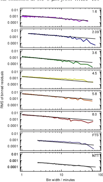
We assessed the presence of correlated noise in the oc-cultation and transit data by plotting the rms of their binned residuals (Figure 2). The 4.5-µm occultation lightcurve and the FTS transit lightcurve each display a small amount of correlated noise on timescales of 5 min and longer.
To obtain a reduced spectroscopic-χ2 of unity and to
balance the different datasets in the MCMC, we added in quadrature a jitter of 14.1 m s−1to the uncertainties of the
CORALIE RVs and 6.9 m s−1 to the uncertainties of the
HARPS RVs, as was done in Hellier et al. (2011).
3.4 Time systems and light travel time
The Spitzer, HAWK-I, FTS and NTT photometry are in the HJD (UTC) time system. The CORALIE and HARPS RVs
Figure 2. RMS of the binned residuals for, from top to bottom, the pre-existing HAWK-I occultation photometry at 1.6 µm and 2.1 µm, the new Spitzer occultation photometry at 3.6, 4.5, 5.8 and 8.0 µm, and the pre-existing FTS and NTT transit photome-try. The solid black lines, which are the rms of the unbinned data scaled by the square root of the number of points in each bin, show the white-noise expectation. The ranges of bin widths are appropriate for the datasets’ cadences and durations.
are in the BJD (UTC) time system. The difference between BJD and HJD is less than 4 s and so is negligible for our purposes, and the timing information mostly comes from the photometry. Leap second adjustments are made to the UTC system to keep it close to mean solar time, so one should really use Terrestrial Time. However, our observations span a short baseline (2008–2010), during which there was only one leap second adjustment, so our choice to use the UTC system has no impact.
The occultation of WASP-19b occurs farther away from us than its transit does, so we made a first order correction for the light travel time. We calculated the light travel time between the beginning of occultation ingress and the begin-ning of transit ingress to be 15 s. We subtracted this from the mid-exposure times of the Spitzer and HAWK-I occul-tation photometry. For comparison, we measure the time of mid-occultation to a precision of 35 s.
3.5 Results
Table 3 shows the median values and the 1-σ uncertainties of the fitted proposal parameters and derived parameters from our final MCMC analysis. Figure 1 shows the best-fitting trend and occultation models together with the raw and detrended Spitzer data. Table 2 gives the best-fitting values for the parameters of the trend models, together with their 1-σ uncertainties. Figure 3 displays all the photometry and RVs used in the MCMC analysis, with the best-fitting eclipse and radial-velocity models superimposed.
Anderson et al. (2010) measured an occultation depth of 0.259 ± 0.045 per cent from their H-band lightcurve. In analysing the same data, we obtained a similar depth of 0.276 ± 0.044 per cent. The minor difference is probably due to some combination of the slightly different manner in how the lightcurves’ error bars were rescaled (see Section 3.3) and the slight difference in the occultation ephemeris (the additional radial-velocity and occultation data result in a mid-occultation time at the time of the H-band observations ∼5 min earlier than found by Anderson et al. (2010)). The occultation depth of 0.366 ± 0.067 per cent that we derived from the 2.09-µm lightcurve of Gibson et al. (2010) is near-identical to the depth that they obtained (0.366 ± 0.072 per cent).
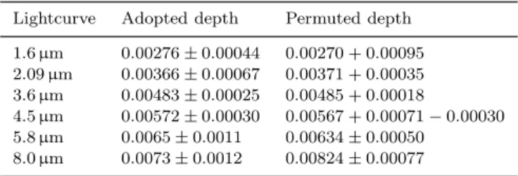
We used the residual permutation or ‘prayer bead’ method (e.g. Gillon et al. 2007) as described in Smith et al. (2012) to assess the impact of any correlated noise present in the occultation lightcurves on our fitted occultation depths. The occultation depths derived from that analysis are con-sistent with the depths we measured from the non-permuted lightcurves and it is the latter that we adopt (Table 4).
We calculated the brightness temperatures that corre-spond to the measured occultation depths and present these in Table 3. To calculate these, we defined the product of the planet-to-star area ratio and the ratio of the band-integrated planet-to-star flux densities, corrected for the wavelength-dependency of the transmission2, to be equal to the
mea-sured occultation depth (e.g., Charbonneau et al. 2005). We used a model spectrum of a star with the Teff, log g and
[Fe/H] values of Table 3 (Hauschildt, Allard & Baron 1999), normalised to reproduce the integrated flux of a black body with Teff = 5475 K. The uncertainties in the brightness
tem-peratures only take into account the uncertainties in the measured occultation depths.
To obtain reliable determinations of the occultation depths and orbital eccentricity, it is important that the time of mid-transit is known with accuracy and preci-sion at the epochs the occultation data are obtained. The WASP photometry, which we used to place a prior on the transit ephemeris, span a two-year baseline of 2006 May to 2008 May and the FTS transit lightcurve was
ob-2 For the HAWK-I measurements, the transmission of
the atmosphere, telescope, instrument, and detector were accounted for by using the transmisson curve obtained from http://www.eso.org/observing/etc/. For the Spitzer measurements, the telescope throughput and detector quantum efficiency were accounted for by using the the full array average spectral response curves available at http://irsa.ipac.caltech.edu/data/SPITZER/docs/
irac/calibrationfiles/spectralresponse/.
Table 4.Comparing adopted and permuted occultation depths
Lightcurve Adopted depth Permuted depth 1.6 µm 0.00276 ± 0.00044 0.00270 + 0.00095 2.09 µm 0.00366 ± 0.00067 0.00371 + 0.00035 3.6 µm 0.00483 ± 0.00025 0.00485 + 0.00018 4.5 µm 0.00572 ± 0.00030 0.00567 + 0.00071 − 0.00030 5.8 µm 0.0065 ± 0.0011 0.00634 ± 0.00050 8.0 µm 0.0073 ± 0.0012 0.00824 ± 0.00077
tained in 2008 December. All occultation data were obtained soon after: during 2009 January to April. The NTT tran-sit lightcurve, obtained in 2010 February, ensured a reli-able transit ephemeris at the occultation epochs. We note, though, that the difference between the transit ephemeris presented herein and that presented in the discovery paper (Hebb et al. 2010, i.e. without the NTT lightcurve), propa-gated to the occultation epochs, is a mere ∼20 s. The ac-curacy of the discovery-paper ephemeris is due to the long baseline of the WASP photometry and the high quality of the FTS lightcurve, which was obtained only months before the occultation data.
3.6 Stellar activity
Hebb et al. (2010) reported a rotational modulation of the WASP lightcurves with a period of 10.5 ± 0.2 days and an amplitude of a few mmag. This indiciated that WASP-19 is an active star, with the sinusoidal modulation being induced by a non-axisymmetric distribution of starspots.
We determine the log R′
HK activity index of WASP-19
by measuring the weak emission in the cores of the Ca iiH+K lines (Noyes, Weiss & Vaughan 1984; Santos et al. 2000; Boisse et al. 2009). The 36 HARPS spectra presented in Hellier et al. (2011) had SNR in the range 14–38. We se-lected the 12 spectra with SNR>19 per pixel at 550 nm, as the activity level tends to be systematically under- or over-estimated for spectra with low SNR. By assuming B − V = 0.570, we infer log R′
HK = −4.50 ± 0.03, which is the
weighted mean and standard deviation of the values de-termined from individual spectra; we used the SNR as the weighting factor. This is similar to the value of log R′
HK =
−4.66 measured by Knutson, Howard & Isaacson (2010). It is difficult to judge the level at which the two values agree as Knutson, Howard & Isaacson (2010) do not provide an uncertainty estimate and our uncertainty value is likely to be an underestimate.
As we know the true stellar rotation period to be 10.5 ± 0.2 days from rotational modulation, we can use our log R′
HK value to test the activity–rotation calibration of
Mamajek & Hillenbrand (2008). The calibration suggests a stellar-rotation period of Prot= 12.3 ± 1.5 d, which is
con-sistent within errors.
We considered whether stellar variability could have af-fected our measured occultation depths. One potential issue is that that the stellar brightness may have varied signif-icantly during one or more of the observations. However, with observation durations of ∼3 hr and a stellar rotation period of 10.5 d, the visible portion of the stellar surface will have changed little during any one observation. To first or-der, the resulting small impact on the occultation lightcurves
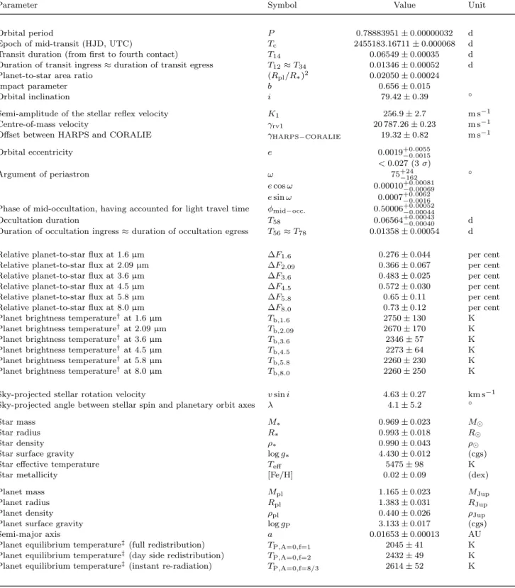
Table 3.System parameters of WASP-19
Parameter Symbol Value Unit
Orbital period P 0.78883951 ± 0.00000032 d
Epoch of mid-transit (HJD, UTC) Tc 2455183.16711 ± 0.000068 d
Transit duration (from first to fourth contact) T14 0.06549 ± 0.00035 d
Duration of transit ingress ≈ duration of transit egress T12≈ T34 0.01346 ± 0.00052 d
Planet-to-star area ratio (Rpl/R∗)2 0.02050 ± 0.00024
Impact parameter b 0.656 ± 0.015
Orbital inclination i 79.42 ± 0.39 ◦
Semi-amplitude of the stellar reflex velocity K1 256.9 ± 2.7 m s−1
Centre-of-mass velocity γrv1 20 787.26 ± 0.23 m s−1
Offset between HARPS and CORALIE γHARPS−CORALIE 19.32 ± 0.82 m s−1
Orbital eccentricity e 0.0019+0.0055−0.0015
< 0.027 (3 σ)
Argument of periastron ω 75+24−162 ◦
e cos ω 0.00010+0.00081−0.00069 e sin ω 0.0007+0.0062−0.0016 Phase of mid-occultation, having accounted for light travel time φmid−occ. 0.50006+0.00052−0.00044
Occultation duration T58 0.06564+0.00043−0.00040 d
Duration of occultation ingress ≈ duration of occultation egress T56≈ T78 0.01358 ± 0.00054 d
Relative planet-to-star flux at 1.6 µm ∆F1.6 0.276 ± 0.044 per cent
Relative planet-to-star flux at 2.09 µm ∆F2.09 0.366 ± 0.067 per cent
Relative planet-to-star flux at 3.6 µm ∆F3.6 0.483 ± 0.025 per cent
Relative planet-to-star flux at 4.5 µm ∆F4.5 0.572 ± 0.030 per cent
Relative planet-to-star flux at 5.8 µm ∆F5.8 0.65 ± 0.11 per cent
Relative planet-to-star flux at 8.0 µm ∆F8.0 0.73 ± 0.12 per cent
Planet brightness temperature† at 1.6 µm T
b,1.6 2750 ± 130 K
Planet brightness temperature† at 2.09 µm T
b,2.09 2670 ± 170 K
Planet brightness temperature† at 3.6 µm T
b,3.6 2346 ± 57 K
Planet brightness temperature† at 4.5 µm T
b,4.5 2273 ± 64 K
Planet brightness temperature† at 5.8 µm T
b,5.8 2260 ± 230 K
Planet brightness temperature† at 8.0 µm T
b,8.0 2260 ± 250 K
Sky-projected stellar rotation velocity v sin i 4.63 ± 0.27 km s−1
Sky-projected angle between stellar spin and planetary orbit axes λ 4.1 ± 5.2 ◦
Star mass M∗ 0.969 ± 0.023 M⊙
Star radius R∗ 0.993 ± 0.018 R⊙
Star density ρ∗ 0.990 ± 0.043 ρ⊙
Star surface gravity log g∗ 4.430 ± 0.012 (cgs)
Star effective temperature Teff 5475 ± 98 K
Star metallicity [Fe/H] 0.02 ± 0.09 (dex)
Planet mass Mpl 1.165 ± 0.023 MJup
Planet radius Rpl 1.383 ± 0.031 RJup
Planet density ρpl 0.440 ± 0.026 ρJup
Planet surface gravity log gP 3.133 ± 0.017 (cgs)
Semi-major axis a 0.01653 ± 0.00013 AU
Planet equilibrium temperature‡ (full redistribution) T
P,A=0,f=1 2045 ± 41 K
Planet equilibrium temperature‡ (day side redistribution) T
P,A=0,f=2 2432 ± 49 K
Planet equilibrium temperature‡ (instant re-radiation) T
P,A=0,f=8/3 2614 ± 52 K
†We modelled both star and planet as black bodies and took account of only the occultation depth uncertainty, which dominates. ‡ T P,A=0,f= f 1 4T eff q R∗
2a where f is the redistribution factor, with f = 1 for full redistribution, f = 2 for dayside redistribution
0.86 0.87 0.88 0.89 0.9 0.91 0.92 0.93 0.94 0.95 0.96 0.97 0.98 0.99 1 1.01 0.4 0.45 0.5 0.55 0.6 Relative Flux Orbital Phase 0.93 0.94 0.95 0.96 0.97 0.98 0.99 1 0.9 0.95 1 1.05 1.1 Relative Flux Orbital Phase -500 -400 -300 -200 -100 0 100 200 300 0.6 0.8 1 1.2 1.4 Relative RV / m s -1 Orbital Phase
Figure 3. The results of our global analysis, which combines our new Spitzer occultation photometry with pre-existing transit photom-etry, ground-based occultation photometry and radial velocities. The models generated from the best-fitting parameter values of Table 3 are overplotted and the residuals about the models are plotted below each dataset. Left: From top to bottom, HAWK-I occultations at 1.6 µm (Anderson et al. 2010) and 2.09 µm (Gibson et al. 2010). The error bar on each binned measurement is the standard deviation of the points within the bin. Top-right: z-band transit lightcurve taken with FTS (top; Hebb et al. 2010) and r-band transit lightcurve taken with NTT (bottom; Hellier et al. 2011). Arbitrary offsets have been applied to the photometry plots for display purposes and Bottom-right: Spectroscopic orbit and transit illustrated by CORALIE and HARPS data (Hebb et al. 2010; Hellier et al. 2011). The measured systemic velocities (Table 3) of each dataset have been subtracted.
can be modelled as a linear trend, which will be handled by the trend functions. Another concern is that the stel-lar brightness may have changed significantly between the non-simultaneous occultation observations. For example, the 3.6-µm data were obtained two months after the 4.5-µm data and it is the relative measurements at these two wave-lengths that are the prime diagnostic for the presence of an atmospheric temperature inversion. Assuming a constant planet brightness, the stellar brightness would need to have changed by ∼5 per cent to have changed the occultation depth by 1 σ and the amplitude of the modulation of the WASP lightcurves (a few mmag) shows that this is very un-likely. Thus our derived eclipse depths, and the conclusions on which they depend, are insensitive to the variability of WASP-19.
4 DISCUSSION 4.1 Atmosphere model
We interpret our observations of the hot Jupiter WASP-19b using the exoplanetary atmospheric modeling and retrieval method developed in Madhusudhan & Seager (2009, 2010, 2011). We model a plane-parallel atmosphere of WASP-19b observed in thermal emission at secondary eclipse. The day-side spectrum of the planet is generated using line-by-line radiative transfer, with constraints of hydrostatic equilib-rium and global energy balance, and includes the dominant sources of infrared opacity expected in gaseous atmospheres at high temperature. Our sources of opacity include molec-ular absorption due to H2O, CO, CH4, CO2, NH3, TiO, and
VO (Freedman, Marley & Lodders 2008; Rothman et al. 2005; Karkoschka & Tomasko 2010) and H2–H2
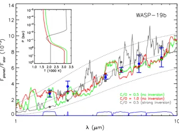
collision-induced absorption (Borysow, Jorgensen & Zheng 1997; Borysow 2002). The concentrations of the species and the pressure–temperature (P –T ) profile constitute the free pa-rameters in the model (Madhusudhan & Seager 2009). We explore the parameter space of the model using a Markov-chain Monte Carlo scheme (see Madhusudhan & Seager 2010, 2011), and constrain regions of parameter space con-sistent with the measured planet-to-star flux density ra-tios at different levels of fit. Our goal is to constrain the existence of a possible temperature inversion, the dayside-to-nightside redistribution efficiency, the concentrations of the different molecular species, and the C/O ratio (e.g. Madhusudhan et al. 2011a) in the dayside atmosphere of WASP-19b. In what follows, we discuss model solutions that explain the data within the 1-σ observational uncertainties, as shown in Fig. 4.
4.2 Temperature inversion
The data indicate the lack of a strong temperature inver-sion in the dayside atmospheres of WASP-19b. The ob-servations and two models fitting the data are shown in Fig. 4. The lack of a temperature inversion in WASP-19b is evident from the data even without detailed modeling. Firstly, the brightness temperature in the 4.5 µm chan-nel, Tb,4.5, is lower than that in the 3.6 µm channel, Tb,3.6
(Table 3). The presence of a temperature inversion is of-ten indicated by a Tb,4.5 value considerably higher than
the Tb,3.6value, due to strong CO emission and some H2O
emission in the 4.5 µm channel (Burrows, Budaj & Hubeny 2008; Fortney et al. 2008; Madhusudhan & Seager 2010). Secondly, the brightness temperatures at 1.6 and 2.09 µm are larger than those in all four IRAC channels, which are at longer wavelengths. Since the bands at 1.6 and 2.09 µm are windows in molecular opacity, they are expected to probe temperatures in deeper layers of the atmosphere compared to any of the IRAC channels. Therefore, the high temper-atures in the 1.6 and 2.09 µm bands compared to all the IRAC channels imply temperature decreasing outwards in the atmosphere, and hence the absence of a temperature inversion or, at most, the presence of one too weak to be detectable with the available data. Two model P –T pro-files without temperature inversions and the corresponding model spectra are shown in Fig. 4. All the IRAC data can be explained by molecular absorption in the atmosphere due to the temperature decreasing outwards.
The lack of a temperature inversion in WASP-19b of-fers a new constraint on existing classification schemes of irradiated giant exoplanets. WASP-19b falls in the category of highly irradiated hot Jupiters which have been predicted to host temperature inversions due to TiO and VO, assum-ing solar abundances (Fortney et al. 2008) - the so called ‘TiO/VO hypothesis’. However, our finding of a lack of a strong temperature inversion in WASP-19b implies that ei-ther TiO and VO are depleted or an entirely different pro-cess is at play. If the composition is oxygen-rich, the lack of a temperature inversion in WASP-19b can be explained if TiO and VO are depleted in the upper atmosphere due to gravitational settling, which can be significant if the vertical mixing is weak (Spiegel, Silverio & Burrows 2009). On the other hand, if the composition is carbon-rich, TiO and VO would be naturally scarce (Madhusudhan et al. 2011b).
Knutson, Howard & Isaacson (2010) posit that the high UV flux impinging on those planets orbiting chromospher-ically active stars could destroy the opacity, high-altitude compounds that would otherwise lead to temper-ature inversions. With log R′
HK = −4.50 ± 0.03,
WASP-19 has a similar activity level to that of the handful of other stars around which hot Jupiters without tempera-ture inversions (log R′
HK = −4.9 to −4.5) are known to
orbit. Those planets thought to have inversions orbit qui-eter stars, with log R′
HK = −5.4 to −4.9. Thus, our
find-ing that WASP-19b has no inversion supports the hy-pothesis of Knutson, Howard & Isaacson (2010) and use-fully adds to the handful of such systems known. Spitzer routinely measures the thermal emission of planets at 3.6 and 4.5 µm. For planets with temperature inversions, CO and water switch from absorption to emission, re-sulting in a higher flux in the 4.5 µm band, in which these molecules have features. Knutson, Howard & Isaacson (2010) proposed a model-independent, empirical metric for classifying hot Jupiters, which we denote with ζ. This is the gradient of the measurements at 3.6 and 4.5 µm, i.e. (∆F4.5− ∆F4.5)/0.9µm, minus the gradient of the black
body that is the best-fit to the two measurements. A positive ζ-value would suggest an inverted atmosphere and a strongly negative ζ-value would indicate a non-inverted atmosphere; Knutson, Howard & Isaacson (2010) suggest a delineation around ζ = −0.05 per cent µm−1. For WASP-19b we
border between inversion and no-inversion and therefore is consistent with our finding that WASP-19b does not have a strong inversion.
We note that in their activity-inversion plot (their figure 5), Knutson, Howard & Isaacson (2010) omit XO-3 but include TrES-4, HAT-P-7 and WASP-18, all of which have Teff & 6200. XO-3b has a temperature inversion and
XO-3 has a log R′
HK index indicative of activity, which
seems to contradict the activity-inversion hypothesis. The other three planets have inversions and orbit quiet stars. Knutson, Howard & Isaacson (2010) concluded that in fact XO-3 is likely to be chromospherically quiet, based on a vi-sual inspection of their spectrum and having noted that the log R′
HK calibration is unreliable for stars with Teff &6200.
Perhaps then TrES-4, HAT-P-7 and WASP-18 are also sus-pect since they also have Teff &6200.
4.3 Atmospheric composition
We find that the observations can be explained by models with oxygen-rich as well as carbon-rich compositions. The absorption in the near-IR (1.6 and 2.09 µm) bands is min-imal due to the lack of major molecular features. The con-straints on the composition come primarily from the IRAC data, which together encompass features of CO, H2O, CH4,
and CO2. The near-IR data, however, are critical to
con-straining the temperature of the lower atmosphere and thus are key in anchoring the model-atmosphere spectra to the measured SED. Two models with different C/O ratios, C/O = 0.5 (oxygen-rich) and C/O = 1 (carbon-rich), are shown in Fig. 4. As demonstrated in Madhusudhan et al. (2011b), CO is a dominant carbon-bearing molecule in both C-rich and O-rich regimes. Consequently, the 4.5 µm absorption in both models in Fig. 4 is caused primarily by CO absorption; in the O-rich model CO2 contributes additional absorption
in this channel. The absorption in the 3.6, 5.8, and 8.0 mi-cron IRAC channels in the O-rich model is caused primarily by H2O absorption, whereas absorption in the C-rich model
is caused by a combination of H2O and CH4 absorption;
H2O is depleted by a factor of 100 and CH4 is enhanced by
a factor of 1000 with respect to the O-rich model, both of which are chemically feasible (Madhusudhan et al. 2011b). The principle difficulty in differentiating between the two models with the current data are the large uncertainties in the 5.8 and 8.0 µm IRAC data. For example, a high 5.8 µm point would indicate low water absorption, and hence high C/O, as demonstrated in Madhusudhan et al. (2011a). New observations in the near infrared can differentiate between spectra from the carbon-rich and oxygen-rich compositions (e.g. Madhusudhan et al. 2011a). The water abundance can be measured via transmission spectoscopy of the 1.4 µm water band using the G141 grism of HST/WFC3; these ob-servations were recently peformed for WASP-19b by Deming (2009). We could measure, or at least place useful constraints on, the TiO abundance with ground-based occultation ob-servations in the z and J bands.
4.4 Orbital eccentricity
For a circular orbit, mid-occultation occurs half an orbital period after mid-transit. We find the occultation to occur
Figure 4.Spectral energy distribution of WASP-19b relative to that of its host star. The blue dots are our fitted planet-to-star flux density ratios. The observation-band transmission curves are shown along the abscissa. The planet-to-star flux density ratios in-dicate the absence of a strong temperature inversion. Two model-atmosphere spectra are shown, each of which fits the data and lacks a temperature inversion. One model has a C/O ratio of 0.5 and is shown as a green line. The other has a C/O ratio of 1.0 is depicted by a red line. The corresponding band-integrated model fluxes are shown as dots with the same colour scheme. The models’ pressure–temperature profiles down to 100 bar are shown in the inset. Assuming zero albedo, the maximum dayside-to-nightside redistribution efficiency is 20 per cent for the C-rich model and 34 per cent for the O-rich model. The three dotted lines show planetary black bodies with temperatures of 1800, 2250 and 2900 K (chosen to give a sense of scale to the spectra) divided by a stellar spectrum.
only 4+35
−30 s later than this and constrain both e cos ω and
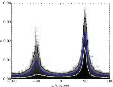
e sin ω to a small region around zero. Hence, the orbit is very nearly circular, though the available data do permit a small, non-zero eccentricity providing that the major axis of the orbit is near-aligned with our line of sight, such that the occulation time is not affected (i.e. |ω| ≈ 90; Figure 5). We place a 3-σ upper limit on eccentricity of e < 0.027.
Hot Jupiters are considered to have been moved inwards to close orbits through planet–planet scattering or by the Kozai mechanism and tidal circularisation (e.g.: Naoz et al. 2011; Wu & Lithwick 2011; Batygin, Morbidelli & Tsiganis 2011). However, for the very shortest-period systems, such as WASP-19b, it is unlikely that they could have been moved directly to their current orbit, since that would have required careful fine-tuning to avoid destruction by collision with the star. Thus most likely WASP-19b was first moved to an orbit near ∼ 2 Roche radii and has since spiralled inwards through tidal orbital decay (see Guillochon, Ramirez-Ruiz & Lin 2011 and the discussion of WASP-19b specifically in Hellier et al. 2011).
From tidal theory, the circularisation of a hot Jupiter’s orbit is thought to proceed much faster than the infall, and this is consistent with the the observation that hot Jupiters tend to be in circular orbits. Thus the suggestion that WASP-19b has undergone significant tidal decay, from ∼ 2 Roche radii to the current 1.2 Roche radii, leads to the expectation that the current eccentricity will be essentially zero, in line with our results.
−180 −90 0 90 180 ω/degrees 0.00 0.01 0.02 0.03 0.04 e
Figure 5. The MCMC posterior distributions of e and ω. The white, blue and black contours are, respectively, the 1-, 2- and 3-σ confidence limits. The shading of each bin is proportional to the logarithm of the number of MCMC steps within. The available data exclude large values of e for any orbital orientation, and only very small values of e are permitted unless |ω| ≈ 90.
ACKNOWLEDGMENTS
This work is based on observations made with the Spitzer Space Telescope, which is operated by the Jet Propulsion Laboratory, California Institute of Technology under a con-tract with NASA. We thank N. P. Gibson for providing the HAWK-I 2.09-µm lightcurve.
REFERENCES
Anderson D. R. et al., 2012, MNRAS, 422, 1988 —, 2011a, A&A, 534, A16
—, 2010, A&A, 513, L3+ —, 2011b, MNRAS, 416, 2108
Barman T. S., Hauschildt P. H., Allard F., 2005, ApJ, 632, 1132
Batygin K., Morbidelli A., Tsiganis K., 2011, A&A, 533, A7
Boisse I. et al., 2009, A&A, 495, 959 Borysow A., 2002, A&A, 390, 779
Borysow A., Jorgensen U. G., Zheng C., 1997, A&A, 324, 185
Burrows A., Budaj J., Hubeny I., 2008, ApJ, 678, 1436 Campo C. J. et al., 2011, ApJ, 727, 125
Charbonneau D. et al., 2005, ApJ, 626, 523
Charbonneau D., Knutson H. A., Barman T., Allen L. E., Mayor M., Megeath S. T., Queloz D., Udry S., 2008, ApJ, 686, 1341
Collier Cameron A. et al., 2007, MNRAS, 380, 1230 Cowan N. B., Agol E., 2011, ApJ, 729, 54
Croll B., Lafreniere D., Albert L., Jayawardhana R., Fort-ney J. J., Murray N., 2011, AJ, 141, 30
de Mooij E. J. W., Snellen I. A. G., 2009, A&A, 493, L35 Deming D., 2009, in HST Proposal 12181
Deming D., Seager S., Richardson L. J., Harrington J., 2005, Nature, 434, 740
D´esert J.-M., Lecavelier des Etangs A., H´ebrard G., Sing D. K., Ehrenreich D., Ferlet R., Vidal-Madjar A., 2009, ApJ, 699, 478
Enoch B., Collier Cameron A., Parley N. R., Hebb L., 2010, A&A, 516, A33+
Fazio G. G. et al., 2004, ApJS, 154, 10 Ford E. B., 2006, ApJ, 642, 505
Fortney J. J., Lodders K., Marley M. S., Freedman R. S., 2008, ApJ, 678, 1419
Freedman R. S., Marley M. S., Lodders K., 2008, ApJS, 174, 504
Fressin F., Knutson H. A., Charbonneau D., O’Donovan F. T., Burrows A., Deming D., Mandushev G., Spiegel D., 2010, ApJ, 711, 374
Gibson N. P. et al., 2010, MNRAS, 404, L114 Gillon M. et al., 2007, A&A, 471, L51
Guillochon J., Ramirez-Ruiz E., Lin D., 2011, ApJ, 732, 74 Hauschildt P. H., Allard F., Baron E., 1999, ApJ, 512, 377 Hebb L. et al., 2010, ApJ, 708, 224
Hellier C., Anderson D. R., Collier-Cameron A., Miller G. R. M., Queloz D., Smalley B., Southworth J., Triaud A. H. M. J., 2011, ApJ, 730, L31+
Ibgui L., Burrows A., Spiegel D. S., 2010, ApJ, 713, 751 Karkoschka E., Tomasko M. G., 2010, Icarus, 205, 674 Knutson H. A., Charbonneau D., Allen L. E., Burrows A.,
Megeath S. T., 2008, ApJ, 673, 526
Knutson H. A., Charbonneau D., Cowan N. B., Fortney J. J., Showman A. P., Agol E., Henry G. W., 2009, ApJ, 703, 769
Knutson H. A., Howard A. W., Isaacson H., 2010, ApJ, 720, 1569
Machalek P., McCullough P. R., Burke C. J., Valenti J. A., Burrows A., Hora J. L., 2008, ApJ, 684, 1427
Madhusudhan N. et al., 2011a, Nature, 469, 64
Madhusudhan N., Mousis O., Johnson T. V., Lunine J. I., 2011b, ApJ, 743, 191
Madhusudhan N., Seager S., 2009, ApJ, 707, 24 —, 2010, ApJ, 725, 261
—, 2011, ApJ, 729, 41
Mamajek E. E., Hillenbrand L. A., 2008, ApJ, 687, 1264 Nagasawa M., Ida S., 2011, ApJ, 742, 72
Naoz S., Farr W. M., Lithwick Y., Rasio F. A., Teyssandier J., 2011, Nature, 473, 187
Noyes R. W., Weiss N. O., Vaughan A. H., 1984, ApJ, 287, 769
Pollacco D. et al., 2008, MNRAS, 385, 1576 Pollacco D. L. et al., 2006, PASP, 118, 1407
Press W., Flannery B., Teukolsky S., Vetterling W., 1992, Numerical Recipes in C: The Art of Scientific Computing. Cambridge University Press
Rothman L. S. et al., 2005, J. Quant. Spec. & Rad. Trans-fer, 139
Santos N. C., Mayor M., Naef D., Pepe F., Queloz D., Udry S., Blecha A., 2000, A&A, 361, 265
Sing D. K., L´opez-Morales M., 2009, A&A, 493, L31 Smith A. M. S. et al., 2012, A&A, 545, A93
Smith A. M. S., Anderson D. R., Skillen I., Collier Cameron A., Smalley B., 2011, MNRAS, 416, 2096
Spiegel D. S., Silverio K., Burrows A., 2009, ApJ, 699, 1487 Werner M. W. et al., 2004, ApJS, 154, 1
Zahnle K., Marley M. S., Freedman R. S., Lodders K., Fort-ney J. J., 2009, ApJ, 701, L20