Génomique des populations et association
génotype-phénotype des écotypes de touladi du lac Supérieur
Mémoire
Alysse Perreault-Payette
Maîtrise en biologie
Maître ès sciences (M. Sc.)
Québec, Canada
© Alysse Perreault-Payette, 2016
Génomique des populations et association
génotype-phénotype des écotypes de touladi du lac Supérieur
Mémoire
Alysse Perreault-Payette
Sous la direction de :
Louis Bernatchez, directeur de recherche
Pascal Sirois, codirecteur de recherche
iii
Résumé
L’apparition et le maintien d’écotypes adaptés à différentes niches écologiques, en situation de sympatrie, est régit par une multitude de facteurs. Ceux-ci sont essentiels pour la compréhension des processus évolutifs impliqués mais aussi pour la gestion et la conservation des populations en question. Le touladi (Salvelinus namaycush) est un salmonidé reconnu pour la présence d’écotypes liée à l’utilisation des ressources et de l’habitat à travers l’Amérique du Nord. Un total de quatre écotypes a été décrit vivant dans le lac Supérieur, se différenciant par l’habitat utilisé, l’alimentation, la morphologie ainsi que l’ostéologie. L’objectif principal de la présente étude était de quantifier l’étendue de la différentiation génétique entre les différents sites d’échantillonnage ainsi qu’entre les différents écotypes. Un second objectif était d’identifier des marqueurs potentiellement sous sélection entre les différents écotypes reflétant de possibles adaptations locales. Pour ce faire, un total de 486 individus, représentant les quatre écotypes pour chacun des quatre sites d’échantillonnages, a été génotypé à 6822 SNPs (polymorphisme de nucléotide simple). De plus, des analyses morphométriques ont été effectuées afin de caractériser l’ampleur de la divergence morphologique entre les écotypes à chacun des sites. Les résultats ont montré une différentiation génétique, bien que faible, plus prononcée entre les sites d’échantillonnage qu’entre les écotypes à chacun de ces sites. Des indices indiquant la présence de sélection divergente ont aussi été décelés entre les écotypes ou en association avec des variations morphologiques, dont certains marqueurs représentant des traits importants dans la divergence des différents écotypes. Les résultats de cette étude permettront une meilleure gestion et conservation des populations de touladi du lac Supérieur en plus d’éclairer le choix possible de populations sources pour l’ensemencement des autres Grands Lacs.
iv
Abstract
Understanding the emergence and maintenance of sympatric ecotypes adapted to various trophic niches is a central topic in evolutionary biology, and also has implications for conservation and management. Lake Trout (Salvelinus namaycush) is renowned for the occurrence of phenotypically distinct ecotypes linked to resource and habitat use throughout North America. A total of four ecotypes have been described in Lake Superior that differ in terms of habitat, diet, morphology and osteology. The principal objective of this study was to quantify the extent of genetic differentiation among sampling sites and among ecotypes. The secondary objective was to identify markers potentially under divergent selection among the four ecotypes that may underlie local adaptation. To this end, a total of 486 individuals were genotyped at 6822 SNPs (single nucleotide polymorphism). In addition, these analyses were conducted alongside morphometric analyses to characterise the extent of morphological divergence among ecotypes within each sampling site. Results reveal that overall genetic differentiation is weak and is higher among sites than among ecotypes within each site. Moreover, we found evidence for divergent selection among ecotypes, and in some instances in association with morphological variation. These markers represent ecologically important traits linked to ecotype divergence. Results from this study will benefit management and conservation practices, and will guide the choice of source populations for stocking in the Great Lakes.
v
Table des matières
Résumé ... iii
Abstract ... iv
Table des matières ... v
Liste des tableaux ... vii
Liste des figures ... viii
Remerciements ... x Avant-propos ... xi Introduction ... 1 L’apparition de nouvelles espèces ... 1 Parallélisme dans la divergence phénotypique... 3 Le touladi ... 4 En Amérique du Nord ... 4 Dans le lac Supérieur ... 5 L’origine et le maintien des écotypes ... 6 Problématique ... 7 Bouleversement du système aquatique ... 7 Plan de réintroduction des poissons de fonds ... 8 Objectifs ... 9
Chapter I: Investigating the Extent of Parallelism in Morphological and Genomic Divergence among Lake Trout Ecotypes in Lake Superior ... 10
Résumé ... 11 Abstract ... 13 Introduction ... 14 Methods ... 17 Results ... 26 Discussion ... 42 Acknowledgements ... 51 Conclusion ... 52 Analyses morphologiques ... 52
vi Analyses génomiques et divergence adaptative ... 53 Différences historiques et impacts anthropogéniques ... 54 Implications pour la gestion et la conservation ... 56 Limitations et perspectives futures ... 57 Bibliographie ... 59 Annexe 1 ... 67
vii
Liste des tableaux
Table 1. Sampling site information and consensus analysis of body shape, head shape and visual
identification. Number of fish sampled per sampling site (N), year of collection and coordinates is provided. Ecotypes were identified by consensus analysis of body shape (B) and/or head shape (H) and/or visual identification (V). Fish for subsequent genetic analysis were chosen based on ecotype consensus. Fish less than 430 mm long were removed prior to the analysis………...….19
Table 2. Models and parameters selected to assign an ecotype to each fish from the four sites
separately. The number of principal components used and the corresponding cumulative percentage of explained variance are in brackets. Models chosen and parameterisation of the covariance matrix are either identified as EII (spherical distribution, equal volume, and equal shape), VEI (diagonal distribution, variable volume, and equal shape), VII (spherical distribution, variable volume, equal shape) or EEI (diagonal distribution, equal volume, and equal shape). The number of groups found (G), the corresponding bayesian information criterion (BIC) and mean uncertainty are also listed for each model….…....29
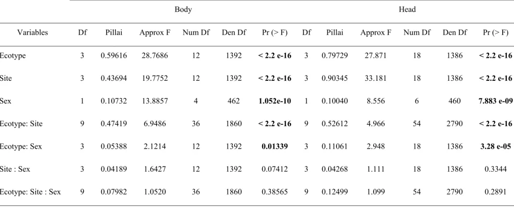
Table 3. MANOVA on body and head shape to investigate the effect of the ecotype, the site of
origin, the sex and all interactions. Significant variables are in bold………..…..…...30
Table 4. Between-group PCA analysis of group distance among ecotypes within and among sites
with 10000 permutation for body (below diagonal) and head (above diagonal) shape. Ecotypes are: Siscowet (FT), Humper (HT), Lean (LT) and Redfin (RF). Group distances with significant p-value (< 0.05) are followed by an asterix (*). Within sites analyses are highlighted in gray and significant between site differences for the same ecotype are in bold. ………..….….31
Table 5. Number of SNPs remaining after each filtration step. Allelic imbalance corresponds to the
ratio of the number of sequences for the major allele on the number of sequences for the minor allele……….…...33
Table 6. Population statistics estimated with 6822 SNPs: the observed heterozygosity (Ho), the
expected heterozygosity (He), the inbreeding coefficient (Gis), the effective population size (Ne) and confidence interval in brackets, and the number of polymorphic loci (N). Genome-wide diversity () and the increase in individual homozygosity relative to mean Hardy-Weinberg expected homozygosity (Fh) was calculated on the dataset prior to filtration. Effective population size for ecotypes with sample size < 15 individuals were not calculated (NA)………..………...35
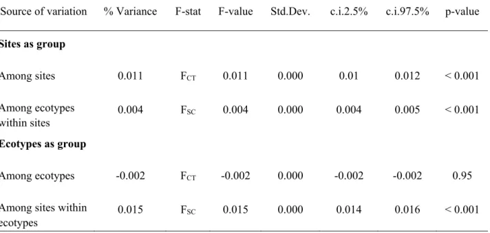
Table 7. Analysis of molecular variance (AMOVA) on 486 individuals and 6822 SNPs. Missing
viii
Liste des figures
Figure 1. Map of Lake Superior sampling sites; Isle Royale, Superior Shoals, Stannard Rock and
Big Reef. Circles correspond to sampling locations for each site……….…….18
Figure 2. Landmark and semi-landmark positions digitized on fish body and head. Homologous
landmarks are represented by red dots and semi-landmarks by black dots. (a) Sixteen homologous landmarks and four semi-landmarks were placed on each fish body; (1) tip of the snout, (2) posterior tip of the maxillary, (3) center of the eye, (4) top of the head above the center of the eye, (5) posterior of neurocranium above the edge of opercula, (6) anterior insertion of dorsal fin, (7) posterior insertion of dorsal fin, (8) anterior insertion of adipose fin, (9) dorsal insertion of caudal fin, (10) midpoint of hypural plate, (11) ventral insertion of caudal fin, (12) posterior insertion of anal fin, (13) anterior insertion of anal fin, (14) anterior insertion of pelvic fin, (15) 50% of body length, (16) 40% of body length, (17) 30% of body length, (18) 20% of body length, (19) anterior insertion of pectoral fin, (20) connection (isthmus) between branchiostegals. (b) Eight homologous landmarks and twenty semi-landmarks were placed on each fish head; (1) tip of the snout, (2-11) ten equally spaced semi-landmarks, (12) posterior edge of the opercula, (13-22) ten equally spaced semi-landmarks, (23) tip of the lower jaw, (24) posterior tip of the maxillary, (25) anterior edge of the eye, (26) center of the eye, (27) posterior edge of the eye, (28) insertion of pectoral fin……….………21-22
Figure 3. Between-group PCA on partial warps of 501 Lake Trout. (a) First and second principal
components for head shape representing 56.2% and 15.9% of the variance respectively distinguishing the four ecotypes. (b) First and second principal components for body shape representing 65.5% and 14.5% of the variance respectively that distinguish leans from siscowets based mainly on belly curvature. (c) Third and fourth principal component for head shape representing 11.5% and 7.2% of the variance respectively distinguishing the four sites. (d) Third and fourth principal components for body shape representing 8.8% and 3.0% of the variance respectively distinguishing the four sites. The colored points refer to the mean scores for each ecotype in each site. The sites are: Big Reef (black), Isle Royale (blue), Stannard Rock (red) and Superior Shoals (green). Ecotypes are: Siscowet (FT), Humper (HT), Lean (LT) and Redfin (RF). Under each ecotype are drawn the consensus shapes of all four ecotypes (gray) with the outline of the ecotype in question (black). The shaded ellipses have been drawn for clarity. ………..32
Figure 4. Population structure analysis of Lake Trout; a) Admixture plot based on 486 individuals
and 6822 SNPs (including outliers) for different values of K. Individuals are shown by sites and ecotypes. b) Neighbour joining tree based on 486 individuals and 6822 SNPs including outliers. Yellow circles represent Big Reef, orange circles Stannard Rock, blue circles Isle Royale and green circles Superior Shoals. Bootstrapping support is indicated on each branch. The four ecotypes are represented for each site; Lean (LT), Humper (HT), Redfin (RF) and Siscowet (FT).………..………38
Figure 5. Assignment success of individuals to their sampling sites (a) or ecotypes (b). Percentage
assignment is written below circles with the exact number of individuals assigned within brackets. Percentage of correct assignment to either sampling sites or ecotypes is in bold.
ix
Sites are: Big Reef (BR), Isle Royale (IR), Stannard Rock (SR), Superior Shoals (SS). Ecotypes are: Humper (HT), Siscowet (FT), Lean (LT) and Redfin (RF).…………..….39
Figure 6. Venn diagrams of outliers detected by LFMM and BAYESCAN among sites, ecotypes or
among ecotypes within sites a) Outliers detected among the four sites by BAYESCAN and LFMM including outliers detected by LFMM using morphological PC scores. b) Outliers detected among the four pooled ecotypes by BAYESCAN and LFMM including outliers detected by LFMM using morphological PC scores. c) Outliers among ecotypes within each site detected by LFMM………...……….…….41
x
Remerciements
Un goût certain pour tout ce qui a trait à la nature a toujours été présent en moi, ainsi qu’un intérêt particulier pour la vie aquatique sous toutes ses formes. Par conséquent, les métiers en relation avec la vie sauvage m’ont toujours attirée et c'est pourquoi j’ai choisi d’étudier dans le domaine de la biologie. C’est également la raison principale de ma venue au Laboratoire du Dr. Louis Bernatchez, titulaire de la chaire de recherche du Canada en génomique et conservation de ressources aquatiques.
J’aimerais le remercier pour m’avoir donné la chance de poursuivre ma passion dans son laboratoire, de même que tous les étudiants, stagiaires et professionnels de recherches présents, sans qui ce projet n’aurait pu être mené à terme. Plus précisément, j’aimerais mentionner, pour leur précieuse collaboration, Cécilia Hernandez pour la partie « laboratoire » du projet, mes collègues de bureau, dont Simon Bernatchez, ainsi que Charles Perrier, Martin Laporte, Jean-Sébastien Moore, Anne-Laure Ferchand, Clément Rougeux, Laura Benestan, Thierry Gosselin et Éric Normandeau pour leurs aides et conseils quant à l’analyse et l’interprétation des résultats.
Ce projet n’aurait pu prendre vie sans le concours et le soutien de la Commission des Pêcheries des Grands Lacs, et tout particulièrement, sans celui de monsieur Andrew Muir. Toute ma reconnaissance à C. Krueger, C. Bronte, M. Hansen et tous les membres de l’équipage du Kiyi pour leur aide lors de l’échantillonnage sur le lac Supérieur. Et c’est sans oublier la collaboration de monsieur Frederick Goetz, de l'Agence américaine d'observation océanique et atmosphérique sans qui l’étude du site « Isle Royale » n’aurait pas été possible.
Finalement, j’aimerais exprimer ma gratitude à ma mère et mon conjoint qui, malgré bien des embûches, ont toujours cru en moi et m’ont encouragée dans cette aventure.
xi
Avant-propos
Vous trouverez, au cœur de ce mémoire, un article intitulé « Investigating the Extent of Parallelism in Morphological and Genomic Divergence among Lake Trout Ecotypes in Lake Superior ». Cet article a été accepté avec corrections mineures par la revue « Molecular Ecology ».
Les co-auteurs sont messieurs Andrew Muir, Frederick Goetz, Charles Perrier et Éric Normandeau, mon co-directeur Pascal Sirois et mon directeur monsieur Louis Bernatchez.
Ont effectué, en grande majorité, le travail de terrain, messieurs Andrew Muir et Frederick Goetz. Ont participé aux analyses, messieurs Éric Normandeau et Charles Perrier, ce dernier ayant aussi travaillé à l’interprétation des résultats. Pour ma part, j’ai réalisé le travail en laboratoire, rédigé l’article, effectué les analyses et interpréter les résultats. De plus, tous les co-auteurs ont collaboré à la révision et l’amélioration du manuscrit.
Ce projet a été rendu possible grâce à la Commission des Pêcheries des Grands Lacs (GLFC) ainsi qu’au regroupement Ressources Aquatiques Québec (RAQ).
1
Introduction
L’apparition de nouvelles espèces
La biodiversité, telle qu’on la connaît aujourd’hui, est le fruit de plusieurs processus évolutifs agissant de concert ou de façon individuelle sur des individus ou des populations. La nature de ces forces soit la mutation, la dérive génétique, la migration, la sélection ainsi que leurs modes d’action, a toujours été au centre de l’étude de l’évolution. On reconnaît maintenant leur importance dans plusieurs autres domaines tels que la gestion et la conservation des ressources. Le processus de spéciation est connu comme étant un moteur de diversité par lequel une espèce se divise en deux ou plusieurs espèces distinctes (Hendry 2009; Weissing et coll. 2011). L’apparition de ces nouvelles espèces est causée par plusieurs forces agissant comme barrières aux flux de gènes entre ces taxons naissants (Turelli et coll. 2001; Hendry 2009). Ces forces prennent la forme d’isolements reproducteurs agissant à plusieurs étapes du cycle de vie, soit avant la reproduction (pré-zygotique) ou directement sur les hybrides produits (post-zygotique). Les barrières pré-zygotiques peuvent être de types écologiques, comportementales, mécaniques ou gamétiques (Schluter 2001; Turelli et coll. 2001) tandis que celles post-zygotiques découlent de la stérilité ou la mortalité des hybrides, ou de leur valeur sélective plus faible en comparaison des parents (Butlin et coll. 2012; Turelli et coll. 2001).
La spéciation est le plus souvent considérée comme un processus graduel où l’accumulation de différences génétiques amène un isolement reproductif (Hendry et coll. 2009). C’est pourquoi, la spéciation est représentée comme un continuum, où à l’une des extrémités, on retrouve des populations présentant des variations adaptatives continues sans aucun isolement reproductif et, à l’autre extrémité, des populations présentant des différences adaptatives accompagnées par un isolement reproductif irréversible (Hendry et coll. 2009). On retrouve donc des populations à différents stades, dits intermédiaires, de ce continuum.
2
La compréhension des facteurs menant à un isolement reproductif et, plus spécifiquement à son niveau d’achèvement, est primordial tant au niveau évolutif qu’au niveau de la conservation (Seehausen et coll. 2008). Par exemple, le niveau d’achèvement de l’isolement reproductif peut déterminer si, lorsque remise en contact, deux populations ou espèces vont fusionner en une seule et même espèce et ainsi perdre les adaptations acquises (Seehausen et coll. 2008).
On retrouve traditionnellement trois modes de spéciation selon le contexte spatial : l’allopatrie, la parapatrie et la sympatrie. L’utilisation et la véracité de ce classement a souvent fait l’objet de débats et de remises en question, mais est encore en vigueur aujourd’hui (Butlin et coll. 2008; Fitzpatrick et coll. 2009). La forme la plus acceptée est celle dite allopatrique, où les populations ou espèces sont séparées par des barrières géographiques empêchant ou réduisant de manière significative la dispersion et, par conséquent, l’échange de gènes (Mallet et coll. 2009). Ce faisant, les populations accumulent des différences génétiques par dérive, ou par des pressions de sélection différentes selon les habitats occupés (Turelli et coll. 2001). Lors d’un contact secondaire, l’accumulation de ces différences pourra mener à un isolement reproductif empêchant complètement ou diminuant le flux génique. Pour sa part, la spéciation dite en parapatrie inclut un certain niveau d’échange de gènes entre les populations seulement à des zones de contacts ou d’hybridation (Butlin et coll. 2012). À l’autre extrémité, on retrouve la spéciation dite en sympatrie où les populations occupent une même région géographique et où tous les individus ont la capacité de se rencontrer physiquement plus ou moins fréquemment (Mallet et coll. 2009). Ce dernier mode de spéciation est causé par la présence d’une sélection divergente liée aux facteurs biotiques et abiotiques présents (Turelli et coll. 2001). Ces facteurs pourraient prendre la forme d’une divergence écologique associée à l’utilisation des ressources et de l’habitat (Blackie et coll. 2003; Hendry 2009).
La présence d’une sélection divergente sur des traits entre populations utilisant différentes ressources et menant à l’isolement reproductif est souvent appelée spéciation écologique (Hendry 2009; Schluter 2016; Gavrilets et coll. 2007). Cette forme de spéciation cause l’apparition d’un certain isolement pré-zygotique sous la forme de sélection sexuelle ou de
3
ségrégation temporelle, et post-zygotique lié à la sélection contre les formes intermédiaires quant à l’exploitation des ressources et à leur compétition (Hendry 2009).
La présence d’un ou de plusieurs phénotypes distincts dans une population utilisant différentes ressources est appelée le polymorphisme des ressources (Wimberger 1994; Skúlason et Smith 1995). Ce polymorphisme peut prendre la forme de différences morphologiques marquées, de différences comportementales ou de traits d’histoire de vie (Skúlason et Smith 1995). On retrouve souvent le polymorphisme des ressources dans un contexte de niche inoccupée et de diminution dans la compétition interspécifique (Skúlason et Smith 1995). Ces conditions, présentes dans les lacs lors du retrait des glaciers, ont été proposées comme moteur dans la radiation adaptative observée chez les poissons d’eau douce en Amérique du Nord. Cette radiation se traduit par la différentiation d’une espèce ancestrale en une série d’espèces adaptées à différentes niches écologiques (Schluter 2001). Un des exemples les plus connus est l’évolution répétée des formes limnétiques et benthiques retrouvées en sympatrie chez plusieurs espèces de poissons telles que le corégone (Coregonus), l’épinoche à trois épines (Gasterosteus aculeatus), et le crapet-soleil (Lepomis gibbosus) et le crapet arlequin (Lepomis macrochirus) (Jonsson 2001; Wimberger 1994; Skùlason et Smith 1995).
Parallélisme dans la divergence phénotypique
Le parallélisme phénotypique, soit l’apparition répétée de phénotypes similaires adaptés à certaines conditions environnementales, a été observé chez plusieurs vertébrés (Elmer et Meyer 2011; Arendt et Reznick 2008). Les outils génomiques modernes permettent maintenant de vérifier si ce parallélisme au niveau phénotypique est suivi d’une base génétique parallèle sous-jacente. Ce parallélisme génétique peut découler du polymorphisme génétique ancestral présent chez l’espèce ou prendre la forme de nouvelles mutations (Elmer et Meyer 2011). Le processus d’adaptation à partir du polymorphisme génétique ancestral est considéré comme plus probable et plus rapide que la mutation pour trois raisons. Premièrement, les allèles sont déjà disponibles, deuxièmement ils sont présents à une plus
4
haute fréquence dans la population, et troisièmement, étant déjà présents, les allèles ont été testés par la sélection et dès lors sont compatibles avec le reste du génome (Barrett et Schluter 2008; Elmer et Meyer 2011). Plusieurs exemples de parallélisme phénotypiques associés à une base génétique similaire ont été documentés chez la souris (Peromyscus polionotus), l’épinoche (Gasterosteus aculeatus), le corégone (Coregonus), les cichlidés et le tétra aveugle (Astyanax mexicanus). Par contre, pour les mêmes espèces énumérées précédemment, une ou plusieurs populations affichant le même phénotype ne montraient pas de parallélisme au niveau génétique et, par conséquent, le phénotype exprimé serait causé par un changement moléculaire différent au courant du développement (Elmer et Meyer 2011; Arendt et Reznick 2008). On peut donc observer au sein d’une même population différente routes évolutives menant à un même phénotype.
Le touladi
En Amérique du Nord
Le touladi est un salmonidé répandu en Amérique du Nord dont la distribution suit les limites de la calotte glacière du Wisconsin, où suivant le retrait des glaciers, il a colonisé les plans d’eau de toutes tailles (Muir et coll. 2015; Wilson et Hebert 1996; Eshenroder 2008). Les populations présentes en Amérique du Nord, proviennent de plusieurs refuges glaciaires, soit ceux de l’Atlantique, du Béringien, du Mississippi, du Montana et du Nahanni (Wilson et Hebert 1998). Ce poisson d’eau douce est reconnu pour sa diversité, comparable à celle de l’Omble chevalier, tant au niveau de la morphologie, des traits d’histoire de vie que de la physiologie et de l’écologie (Muir et coll. 2015). L’apparition répétée de formes adaptées à l’eau peu profonde ou ayant des adaptations liées à un mode de vie en eau profonde a été répertoriée dans plusieurs lacs nord-américains (Muir et coll. 2015). Par exemple, on retrouve deux écotypes dans le lac Mistassini et le lac Rush, dont l’un adapté à la vie en eau peu profonde et l’autre aux eaux profondes (Zimmerman et coll. 2007; Muir et coll. 2015). Il est à noter que dans des lacs de plus grande superficie, on peut retrouver jusqu’à quatre
5
écotypes différents. Par exemple, jusqu’à quatre écotypes adaptés aux eaux peu profondes ont été trouvé au Grand lac de l’Ours (Harris et coll. 2014; Muir et coll. 2015), tandis qu’au Grand lac des Esclaves, on retrouve un écotype adapté aux eaux peu profondes ainsi que deux adaptés aux eaux profondes (Zimmerman et coll. 2006; Muir et coll. 2015).
Dans le lac Supérieur
Dans le lac Supérieur, on retrouve quatre écotypes de touladi : le « lean » dit maigre, le « siscowet » dit gras, le « humper » dit bossu et le « redfin » (Muir et coll. 2014). Ces écotypes diffèrent principalement au niveau de l’habitat, de l’alimentation, de la morphologie et dans certains traits d’histoire de vie, tels que la croissance et la taille à la maturité (Muir et coll. 2015). Le maigre est le seul écotype exploité par la pêche commercial et récréative en raison du faible taux de lipides présent dans ses tissus (Bronte et Sitar 2008). Cet écotype est décrit comme ayant une forme allongée, un museau droit et pointu ainsi qu’un long pédoncule caudal lui permettant de nager de manière prolongée (Burnham-Curtis & Smith 1994; Moore & Bronte 2001; Zimmerman et coll. 2006). On le retrouve en eaux peu profondes (< 100 m) près des côtes où il se nourrit de petites espèces de poissons pélagiques ou de fond tels que l’éperlan arc-en-ciel (Osmerus mordax), le cisco de lac (Coregonus artedi) et le chabot visqueux (Cottus cognatus) (Goetz et coll. 2011; Ray et coll. 2007; Zimmerman et coll. 2006). À l’opposé, l’écotype gras est le plus abondant et on le retrouve principalement en eaux profondes (> 100 m) au large des côtes (Bronte et coll. 2003; Ray et coll. 2007; Goetz et coll. 2011). Cet écotype est décrit comme ayant un corps robuste et épais, une tête plutôt petite, un museau court et incliné ainsi que de grands yeux. Il est aussi reconnu pour avoir un pédoncule caudal épais et long ainsi que de grandes nageoires lui permettant d’effectuer de soudaines poussées de vitesse pour attraper ses proies. De plus, l’écotype gras tient son nom du niveau élevé de lipides dans ses viscères lui donnant une flottabilité plutôt neutre, et par le fait même, facilitant les migrations verticales dans la colonne d’eau à la poursuite de ses proies. Celles-ci sont composées principalement de corégoninés (corégones, ciscos, ménominis), de chabots de profondeur (Myoxocephalus thompsoni) et de lottes (Lota lota) (Goetz et coll. 2011; Ahrenstorff et coll. 2011; Hrabik et
6
coll. 2014; Bronte et coll. 2003; Bronte and Sitar 2008; Burnham-Curtis and Smith 1994; Hansen et coll. 2012). Habitant les hauts-fonds au large des côtes, l’écotype bossu est peu répandu dans le lac Supérieur (Zimmerman et coll. 2006). On le reconnaît à sa petite taille, à sa petite tête ayant un museau incliné et de grands yeux, à une paroi abdominale plutôt mince ainsi qu’à un niveau de lipides intermédiaire (Bronte et coll. 2003; Goetz et coll. 2011; Moore et Bronte 2001). C’est le seul écotype qui ne soit pas piscivores à l’âge adulte, se nourrissant principalement de Mysis diluviana (Stafford et coll. 2014). Finalement, l’écotype « redfin » a été décrit récemment près de l’Isle Royale dans la partie ouest du lac Supérieur (Muir et coll. 2014). Il est décrit comme ayant un corps robuste, une tête, un museau et des yeux larges, un pédoncule caudal long et épais ainsi que de grandes nageoires (Muir et coll. 2014). On le retrouve en eaux de profondeur moyenne (~ 80 m) et il semble avoir un niveau de lipides semblable et même plus élevé que l’écotype gras (Muir et coll. 2014; Hansen et coll. 2016). De plus, il est de plus grande taille, plus lourd, plus longévif et a une croissance plus lente que les autres écotypes à l’Isle Royale (Hansen et coll. 2016).
L’origine et le maintien des écotypes
Plusieurs hypothèses ont été avancées pour expliquer la présence de ces écotypes dans le lac Supérieur (Wilson et Mandrak 2004; Eshenroder 2008). La première est la plasticité phénotypique induite par l’environnement qui se traduit par l’apparition de plusieurs phénotypes à partir d’un seul génotype selon des variations biotiques ou abiotiques. La deuxième hypothèse sous-entend la présence d’une base génétique entre les différents écotypes, et donc d’un certain isolement reproductif (Goetz et coll. 2010). Plusieurs évidences pointent vers la deuxième hypothèse, soit la présence d’une base génétique, pour expliquer l’apparition et le maintien des écotypes. En premier lieu, les écotypes (maigre, bossu, et gras) diffèrent au niveau de certains os crâniens, plus spécifiquement au niveau de la forme de l’opercule, du supraethmoïde ou du dermethmoïde. Des variations environnementales ou ontogéniques sont peu plausibles pour expliquer les différences morphologiques observées avec ces os (Burnham-Curtis et Smith 1994). De plus, la progéniture des écotypes maigres et gras a été élevée en milieu contrôlé et retenait la plupart des traits distinctifs les séparant (Goetz et coll. 2010). La même étude a aussi décelé des
7
différences au niveau de l’expression de certains gènes, entre ces écotypes, associés au métabolisme des lipides. Aussi, deux études utilisant des microsatellites ont montré, bien que faiblement, une plus grande variance liée aux écotypes qu’aux localités (Page et coll. 2004; Guinand et coll. 2012). Par contre, plusieurs études ont démontré un schéma contraire, soit une plus grande variance liée aux sites d’échantillonnage qu’aux écotypes (Dehring et coll. 1981; Ihssen et coll. 1988; Baillie et coll. 2016). L’homogénéisation génétique et phénotypique des écotypes de touladi, vivant dans le lac Supérieur, a été avancée pour expliquer la présence d’une plus grande différentiation génétique entre les sites d’échantillonnage qu’entre les écotypes (Baillie et coll. 2016). En effet, en étudiant des échantillons préeffondrements et contemporains, Baillie et collaborateurs (2016) ont identifié un regroupement génétique par écotypes plus importants chez les individus préeffondrements que chez les individus contemporains qui se regroupent majoritairement par site d’échantillonnage. La surpêche, l’ensemencement intensif et l’introduction d’espèces invasives ont été énoncés pour expliquer le plus grand échange de gènes, observé aujourd’hui, entre les différents écotypes (Baillie et coll. 2016).
Problématique
Bouleversement du système aquatique
Jusqu’à dix variétés de touladis ont été décrites de manière anecdotique par les pêcheurs du lac Supérieur, selon des distinctions au niveau de l’apparence physique, de l’habitat et du comportement. Celles-ci étaient exploitées commercialement, tout particulièrement la forme maigre dû à son faible taux en lipides (Goodier 1981; Bronte et Sitar 2008). Dans les années 1960, la pêche s’est effondrée et le touladi a disparu des Grands Lacs à l’exception du lac Supérieur et d’une partie du lac Huron (Bronte et Sitar 2008). Cet effondrement a été causé principalement par l’activité humaine, dont la surpêche, la dégradation de l’habitat et l’introduction d’espèces envahissantes notamment la lamproie marine (Bronte et Sitar 2008; Page et coll. 2003; Page et coll. 2004). En ce qui a trait aux salmonidés, six espèces ont été introduites dont la truite brune et arc-en-ciel, ainsi que les saumons chinook, coho, rose et
8
atlantique. Elles ont été introduites afin de diversifier et d’augmenter la pêche sportive, mais ont eu pour effet de changer la dynamique des poissons-fourrages ainsi que de leurs prédateurs (Bronte et coll. 2003). Le contrôle de la lamproie marine et l’ensemencement intensif ont permis de restaurer les stocks de touladis dans le lac Supérieur, mais bien en deçà des niveaux historiques (Bronte & Sitar 2008). Malgré plusieurs efforts de restauration dans les autres Grands Lacs, aucune population reproductrice autonome n’a pu être créée dans ces derniers (Page et coll. 2003).
Plan de réintroduction des poissons de fonds
Le rétablissement des poissons de fonds tels que le touladi dans les Grands Lacs est encore incertain et a fait l’objet d’un article par deux biologistes de la Commission des Pêcheries des Grands Lacs (Zimmerman et Krueger 2009). Ceux-ci ont examiné plusieurs facteurs pouvant freiner ou empêcher son rétablissement dans les Grands Lacs. À cet effet, quatre sujets de recherche ont été désignés comme capitaux, soient :
− une plus grande compréhension des variations spatiales et temporelles liées au recrutement,
− l’identification de la ou des sources de mortalité des premiers stades de vie,
− la comparaison de l’histoire de vie et de l’écologie de l’écotype maigre avec ceux des autres écotypes, et
− la détermination du niveau de différentiation génétique entre les écotypes et les populations.
La diversité génétique est associée au potentiel évolutif d’une espèce face aux changements (Toro et Caballero 2005). C’est ainsi que le maintien d’une grande diversité génétique, ainsi qu’une grande diversité phénotypique, augmenterait la résilience et la résistance des espèces face aux changements dans l’environnement. Donc, l’établissement d’une combinaison de populations adaptées à divers habitats devrait augmenter la résilience du touladi dans un même plan d’eau (Zimmerman et Krueger 2009).
L’utilisation d’outils génomiques de pointe ainsi que des approches pangénomiques permettrait d’augmenter la résolution génétique entre les différents écotypes, et ce faisant de
9
préciser les mécanismes soutenant l’origine et le maintien des écotypes de touladi dans le Lac Supérieur. De plus, un échantillonnage à plusieurs sites connus pour l’abondance de cette espèce permettrait de déterminer la connectivité génétique à travers le lac, mais aussi de vérifier la présence de variabilité génétique liée à la localité.
Objectifs
L’objectif principal de cette étude était d’approfondir les connaissances quant à l’origine et l’ampleur de la différentiation génétique des différents écotypes de touladi dans une optique de gestion et de conservation. Afin d’atteindre cet objectif, deux cibles spécifiques ont été identifiés soit : (i) de documenter et comparer l’étendue de la structure et de la connectivité génétique entre les différents écotypes et entre les différents sites d’échantillonnage et (ii) d’identifier de possibles divergences adaptatives incluant les associations génotype-phénotype entre les différents écotypes.
10
Chapter I: Investigating the Extent of Parallelism in
Morphological and Genomic Divergence among
Lake Trout Ecotypes in Lake Superior
Chapitre I: Évaluation de l’étendue du parallélisme dans la divergence morphologique
et génomique des écotypes de touladi du lac Supérieur
11
Résumé
Comprendre le processus de spéciation écologique par lequel de nouvelles espèces émergent est au centre de la biologie évolutive, mais il est tout aussi important en ce qui a trait à la conservation et la gestion. Le touladi (Salvelinus namaycush) est reconnu pour la présence d’écotypes associés à l’utilisation de l’habitat et des ressources à travers l’Amérique du Nord. Nous avons utilisé le séquençage de nouvelle génération afin de définir la structure génétique fine des quatre écotypes de touladis décrits dans le lac Supérieur, le plus grand lac en Amérique du Nord. Pour ce faire, 486 individus provenant des quatre écotypes présents en sympatrie à quatre sites d’échantillonnage ont été génotypés à 6822 SNPs en utilisant la technologie de séquençage « RAD ». De plus, les traits phénotypiques de tous les individus séquencés ont été documentés sous la forme d’analyses morphométriques conjointes de la forme de la tête et du corps ainsi qu’une identification visuelle. Les résultats obtenus ont révélé la présence de différents niveaux de différentiation morphologique et génétique à l’intérieur des différents sites. De manière générale, la différentiation génétique était faible, mais significative et était en moyenne près de trois fois plus prononcées entre les sites (FST Moyen = 0.016 [0.012; 0.021]) qu’entre les écotypes à chacun de ces sites (FST Moyen= 0.005 [0.004; 0.007]). Ceci indique un flux de gènes plus important ou un ancêtre commun plus récent à l’intérieur de chaque site, qu’entre les populations du même écotype. Malgré, le peu d’indication quant à la présence d’une origine commune des différentes populations appartenant à chaque écotype, des individus correspondant à la description des différents écotypes ont été identifiés à chacun des sites, ce qui suggère une convergence dans les traits phénotypiques. Des indices de la présence de sélection divergente ont été trouvés entre les écotypes ou en association avec des variations morphologiques. En effet, plusieurs marqueurs associés au métabolisme des lipides ainsi qu’à l’acuité visuelle sont particulièrement intéressants dans un contexte de divergence entre les écotypes. Globalement, la présence de différents niveaux de différentiation génomique entre les écotypes à chacun des sites ainsi que la présence de loci différentiés associés à des fonctions
12
biologiques d’intérêt supportent un scénario de divergence répété des différents écotypes en sympatrie, à l’intérieur de chaque localité.
13
Abstract
Understanding the emergence of species through the process of ecological speciation is a central question in evolutionary biology which also has implications for conservation and management. Lake Trout (Salvelinus namaycush) is renowned for the occurrence of different ecotypes linked to resource and habitat use throughout North America. We used next generation sequencing to unravel the fine genetic structure of the four Lake Trout ecotypes described in Lake Superior. A total of 486 individuals from four sites where the four ecotypes occur in sympatry were genotyped at 6822 filtered SNPs using RADseq technology. Phenotypic traits of all sequenced fish were documented using a combination of morphometric analyses. Our results revealed different extent of morphological and genetic differentiation within the different sites. Overall, genetic differentiation was weak but significant and was on average three times higher between sites (Mean FST = 0.016) than between ecotypes within sites (Mean FST = 0.005) indicating higher level of gene flow and/or a more recent shared ancestor between ecotypes within each site than between populations of the same ecotype. Evidence of divergent selection was also found between ecotypes and/or in association with morphological variation. Outlier loci found in gene related to lipid metabolism and visual acuity were of particular interest in this context of ecotypes divergence. Overall, the occurrence of different levels of both genomic and phenotypic differentiation between ecotypes within each site with several differentiated loci linked to relevant biological functions support the presence of a continuum of divergence in Lake Trout.
14
Introduction
The study of diversification and ultimately speciation is central to evolution and relevant for conservation biology (Weissing et al. 2011). The most common and established mechanism of speciation is divergence in allopatry, where spatial and geographical barrier prevent gene flow, thus allowing genetic incompatibilities to accumulate, subsequently resulting in reproductive isolation following secondary contact (Coyne and Orr 2004; Tittes and Kane 2014). Some examples of allopatric isolation mechanisms in fishes include the glacial cycles in North America responsible for the origin of many freshwater species (April et al. 2013), the rise and fall of Lake Tanganyika, and the barriers created by high water flow in large rivers such as the Amazon or Congo River (reviewed in Bernardi 2013). However, a geographic barrier is not always needed and speciation can emerge in sympatry, or in parapatry despite high gene flow, by divergent selection on ecologically important traits (Tittes and Kane 2014; Gavrilets et al. 2007). Divergent selection on ecological traits can be caused by biotic and abiotic influences where adaptations to different environment or ecological niches result in the emergence of reproductive incompatibilities (Bernardi 2013; Nosil et al. 2009). The latter may create a continuum of divergence from continuous variation within a single gene pool, to ecotype formation and finally to complete differentiation and reproductive isolation (Lu and Bernatchez 1999; Nosil et al. 2009; Hendry 2009). Models and case studies have shown that sympatric speciation is possible under gene flow when few loci underlying the divergent trait undergo strong selection, whereas gene flow homogenises the rest of the genome (Gavrilets et al. 2007; Franchini et al. 2013).
Ecological speciation has been extensively documented in several geologically young fish species living in sympatry. For instance sympatric speciation has occurred in Midas cichlids (Amphilophus spp.) (Franchini et al. 2013), Lake Victoria cichlids (Wagner et al. 2013) but more commonly in several temperate freshwater fishes such as stickleback (Gasterosteus spp.), smelt (Osmerus spp.) and mainly in salmonids such as whitefish (Coregonus spp.), trout (Salmo spp.), Pacific salmon (Oncorhynchus spp.) and charrs (Salvelinus spp.) (Taylor 1999; Jonsson and Jonsson 2001). Sympatric speciation is usually linked to trophic
15
polymorphism in which intra-specific ecotypes use different habitats and resources (Blackie et al. 2003; Hansen et al. 2012; Smith and Skúlason 1996). Trophic polymorphism is common in post-glacial lakes where retreat of the ice sheet creates unoccupied niches and opportunities for intra-specific competition (Blackie et al. 2003; Zimmerman et al. 2009). These conditions are believed to be responsible for the extensive radiation in North American freshwater fishes where several species are adapted to different ecologic niches (Schluter 2001). Parallel evolution of shared phenotypic traits linked to trophic resource use has been demonstrated in several postglacial systems. These shared morphological traits between populations can be accompanied by shared genetic architecture underlying the ecologically important traits or can arise from independent genetic processes (Ralph and Coop 2014). For example, the repeated divergence of marine and freshwater stickleback exhibiting similar phenotypic changes in body armour have been described and the repeated reduction in armour plates was found to be controlled by the same set of loci (Colosimo et al. 2005; Jones et al. 2012). On the other hand, convergent phenotypic traits may not always be controlled by similar developmental pathways as is the case for cavefish (Astyanax spp.), beach mice (Peromyscus polionotus), and fruit fly (Drosophila spp.) (reviewed in Arendt and Reznick 2008; Bernatchez (submitted)). For instance, the evolution of parallel phenotypic divergence between benthic normal and limnetic dwarf whitefish (Coregonus spp.) in several North American lakes was found to be only partially associated with parallelism at the genome level (Gagnaire et al. 2013; Laporte et al. 2015).
Lake Trout (Salvelinus namaycush) are renowned for the occurrence of different ecotypes linked to resource and habitat use throughout North America. In small lakes, Lake Trout diverged mainly into a planktivorous and piscivorous ecotype (Vander Zander et al. 2000), whereas several large lakes harbor at least four ecotypes associated with differential resource partitioning (Muir et al. 2015). For instance, four different ecotypes occur in Great Bear Lake and Lake Superior, three in Great Slave Lake and two in Lake Mistassini and Rush Lake (Muir et al. 2015). In Lake Superior, four distinct ecotypes have been reported that are recognized based on differences in morphology and coloration but also in life history traits, physiology and ecology (Muir et al. 2015). For instance, they differ in traits such as growth rate, asymptotic length and weight, size at sexual maturity, as well as developmental rate of
16
fertilized eggs or fry. They also differ in physiology such as buoyancy and swim bladder retention (Muir et al. 2015; Hansen et al. 2016). The ‘lean’ ecotype has a slender, streamlined body with low body lipid content, and occupies shallow waters where it preys upon pelagic fishes (Bronte et al. 2003; Goetz et al. 2011; Burnham-Curtis and Smith 1994; Moore and Bronte 2001; Zimmerman et al. 2009). The ‘humper’ ecotype inhabits offshore, mid-water shoals, feeds on small prey and is sexually mature at relatively smaller sizes (< 500 mm) (Stafford et al. 2014; Burnham-Curtis and Smith 1994; Hansen et al. 2016). It also has a small head with moderately large eyes dorsally positioned and short-paired fins (Zimmerman et al. 2009; Moore and Bronte 2001; Bronte et al. 2003). The ‘siscowet’ ecotype is recognized by its sloping snout, moderately large eyes and high body fat content which may facilitate diel vertical migration to follow the migration of ciscoes (Ahrenstorff et al. 2011; Hrabik et al. 2014; Bronte et al. 2003; Bronte and Sitar 2008; Burnham-Curtis and Smith 1994; Hansen et al. 2012). Lastly, the ‘redfin’ ecotype has a robust body, a large head, a long deep peduncle and large fins (Muir et al. 2014). Several hypotheses have been proposed to explain the origin of these ecotypes (Wilson and Mandrak 2004; Eshenroder 2008). These could be the result of developmental plasticity in which a single genotype expresses different phenotypes matching selection optima or can be genetically based or a mix of both (Goetz et al. 2010). While this does not rule out a role for developmental plasticity, two lines of evidence suggest some genetic basis for the phenotypic differences observed between the ecotypes. First, progeny from wild lean and siscowet gametes have been raised in a common garden experiment and key phenotypic features that differentiate wild leans and siscowets such as condition factor, morphology and lipid content were maintained (Goetz et al. 2010). Furthermore, the same study uncovered transcriptional differences in lipid-related genes between the two ecotypes (Goetz et al. 2010). Second, morphological differences in the operculum and supraethmoid bones have been documented between leans, siscowets and humpers. Cranial bones are of taxonomic significance in salmonids and are unlikely affected by environmental conditions and ontogenic shifts (Burnham-Curtis and Smith 1994).
Lake Trout (Salvelinus namaycush) were once the dominant predator in the Great Lakes. It historically supported one the most important freshwater commercial fisheries before being
17
extirpated in the 1950s in all lakes except Lake Superior, where it is now considered restored and Lake Huron, where recruitment has been increasing (Riley et al. 2007), but it remains at relatively low abundance (Zimmerman and Krueger 2009, Bronte et al. 2003). The collapse of Lake Trout populations has been associated with anthropogenic factors, including habitat degradation, pollution and overfishing, as well as predation by invasive sea lamprey following the construction of navigation canals (Bronte and Sitar 2008; Page et al. 2003; Page et al. 2004). Impediments to its recovery or restoration have been the object of a review by Zimmerman and Krueger 2009 and guidelines have been provided to maintain, increase or reintroduce Lake Trout population in the Laurentian Great Lakes. Understanding and evaluating genetic structure and diversity of remaining Lake Trout population has been identify as key research topic.
The general goal of this study was to gain insight into the nature and origin of the different Lake Trout ecotypes in Lake Superior. More specifically, we aimed to; 1) investigate the extent of both morphological and genome wide genetic differentiation and connectivity among the four Lake Trout ecotypes from different geographic locations within the lake; and 2) identify possible adaptive genetic differentiation among ecotypes by means of genome scans and genotype-phenotype associations. To achieve this, we used RADseq to genotype Lake Trout from the four ecotypes and from four sites from Lake Superior. In parallel, geometric morphometric analyses were performed on head and body shape.
Methods
Sampling
Fish from the four Lake Trout ecotypes were sampled in 2013-2014 from four sites in Lake Superior; Big Reef (2014), Stannard Rock (2013-2014), Superior Shoals (2013) and Isle Royale (2013) (Figure 1, Table 1). For the first three sites, a nylon gill net, 183 m long by 1.8 m high, was used with 30.5 m long panels of different mesh sizes (50.8-114.3 mm). Nets were deployed for 24 hours at different depth ranges (0-50 m, 50-100 m and >100 m) approximately representing preferred depths of the different ecotypes. A picture of each fish
18
was taken following the protocol in Muir et al. (2012) and a biopsy of either the adipose or pectoral fin was collected and preserved in 95% ethanol. The fourth site, Isle Royale, was sampled in 2013 using overnight sets of 274-823 m long gill nets with nine panels (91.4 m long by 1.83 m high) of single mesh size (5.1 cm, 6.4 cm, 7.6 cm, 8.9 cm, 10.2 cm, 11.4 cm, 12.7 cm, 14.0 cm, 15.2 cm). Pictures were taken using the same protocol (Muir et al. 2012) and liver or gonads were conserved in RNA Later. Samples without pictures or genetic material were removed from subsequent analyses. Information about total length (mm), wet weight (g) and sex, and depth of capture were recorded for each sampled individual.
Figure 1. Map of Lake Superior sampling sites; Isle Royale, Superior Shoals, Stannard Rock and
19
Table 1. Sampling site information and consensus analysis of body shape, head shape and visual identification. Number of fish sampled per sampling site (N), year of collection and coordinates is provided. Ecotypes were identified by consensus analysis of body shape (B) and/or head shape (H) and/or visual identification (V). Fish for subsequent genetic analysis were chosen based on ecotype consensus. Fish less than 430 mm long were removed prior to the analysis.
Sites Year Coordinates N
Lean-like Siscowet-like Humper-like Redfin-like no consensus Total Big Reef 2014 46°46,545°N 86°28,378°W 132 Consensus 39B, H,V 46B, H, V 8V 17V 13 123 Chosen 39 40 8 17 104 Stannard Rock 2013-2014 47°11,450°N 87°11,531°W 362 Consensus 63B, H, V 66 B, H, V 24V 24V 40 217 Chosen 40 40 24 24 128 Isle Royale 2013 47°21,550°N 88°30,497°W 214 Consensus 55B, H, V 37B, H, V 35H,V 33B, V 42 202 Chosen 40 37 34 33 144 Superior Shoals 2013 48°02,464°N 87°07,536°W 394 Consensus 35B, H, V 133B, H, V 11V 62B, V 74 315 Chosen 31 41 11 42 125
20 1
Ecotype assignment 2
Consensus of both morphometric analyses (body and head) and visual identification as 3
visual interpretation of fish pictures by Lake Trout experts (see Acknowledgements) was 4
used to assign an ecotype to each fish per Muir et al. (2014). Fish less than 430 mm long 5
with the exception of humper-like fish, that are < 430 mm when sexually mature, were 6
excluded to remove the confounding effect of ontogenetic shifts in morphology 7
(Zimmerman et al. 2009). Body and head were analysed separately to distinguish 8
locomotion (body) from feeding habit (head). In addition, morphometric analyses were 9
conducted separately for each site to investigate morphological variation among sites. 10
Landmarks and semi-landmarks were digitized and analysed with the Thin Plate Spline suite 11
(TPS; State University of New York at Stony Brook; http://life.bio.sunysb.edu/morp). First, 12
for each fish a rectangular grid was overlaid to identify belly curvature corresponding to 20-13
30-40-50% of body length using the program REVIT (Autodesk) (Figure 2a). The body grid 14
was anchored at the tip of the snout and the midpoint of the hypural plate. Second, 16 15
homologous landmarks and four semi-landmarks were digitized on each fish with the 16
program TpsDig2 and semi-landmarks were slid using TpsUtil (Figure 2a). Semi-landmarks 17
were used to represent belly curvature which is known to be distinctive between the two 18
major ecotypes, leans and siscowets (Muir et al. 2014). Similarly, a squared grid was 19
overlaid on each fish head dividing it into 10 equally spaced sections using the program 20
REVIT (Figure 2b). The head grid was anchored at the tip of the snout and the posterior 21
edge of the opercula. Eight homologous landmarks and 20 semi-landmarks were digitized on 22
each fish head with the program TpsDig2 and semi-landmarks were slid using TpsUtil 23
(Figure 2b). Distortions from rotation and size were removed by the program TpsRelw 24
producing partial warps scores which are size-free variables. A principal component analysis 25
(PCA) was performed to reduce the number of morphometric variables or scores and extract 26
divergent morphometric patterns. Subsequently, relevant axes were supplied to a Bayesian 27
clustering analysis implemented in the R package Mclust v.4. Mclust is a normal mixture 28
modeling for model-based cluster analysis, classification and density estimation that include 29
the Bayesian Information Criterion (BIC) for model selection and that do not require priori 30
information about groups such as discriminant function analysis (Fraley & Raftery 2012). 31
21
Components accounting for more than 65% of the variance were supplied to the Mclust 32
algorithm. The best model was the one with the highest BIC able to separate leans from 33
siscowets since they are the most morphologically differentiated ecotypes (Fraley and 34
Raftery 2012; Muir et al. 2014). Group classification resulting from the chosen model was 35
retrieved for each individual. The visual identification of each collected fish from Big Reef, 36
Stannard Rock and Superior Shoals was conducted by visual consensus of three trained 37
biologists. Visual identification of Isle Royale fish was provided by an experienced 38
biologist. An ecotype was assigned to each fish based on the consensus from body shape, 39
head shape and visual identification. Two out of three similar ecotype assignments were 40
needed to assign to each fish a particular ecotype. In the case of different head, body and 41
visual assignations; the fish were assigned « no consensus» and removed from subsequent 42
analyses. Fish for subsequent genetic analyses were chosen as follow: (1) fish with 100% 43
consensus having the lowest group uncertainty and (2) fish with 2/3 consensus having the 44
lowest group uncertainty. However, if an ecotype was not identified based on morphometric 45
analysis, the visual identification only was used and taken into account in subsequent 46 analyses. 47 48 49 a)
22 50
Figure 2. Landmark and semi-landmark positions digitized on fish body and head. Homologous
51
landmarks are represented by red dots and semi-landmarks by black dots. (a) Sixteen homologous 52
landmarks and four semi-landmarks were placed on each fish body; (1) tip of the snout, (2) posterior 53
tip of the maxillary, (3) center of the eye, (4) top of the head above the center of the eye, (5) posterior 54
of neurocranium above the edge of opercula, (6) anterior insertion of dorsal fin, (7) posterior 55
insertion of dorsal fin, (8) anterior insertion of adipose fin, (9) dorsal insertion of caudal fin, (10) 56
midpoint of hypural plate, (11) ventral insertion of caudal fin, (12) posterior insertion of anal fin, 57
(13) anterior insertion of anal fin, (14) anterior insertion of pelvic fin, (15) 50% of body length, (16) 58
40% of body length, (17) 30% of body length, (18) 20% of body length, (19) anterior insertion of 59
pectoral fin, (20) connection (isthmus) between branchiostegals. (b) Eight homologous landmarks 60
and twenty semi-landmarks were placed on each fish head; (1) tip of the snout, (2-11) ten equally 61
spaced landmarks, (12) posterior edge of the opercula, (13-22) ten equally spaced semi-62
landmarks, (23) tip of the lower jaw, (24) posterior tip of the maxillary, (25) anterior edge of the eye, 63
(26) center of the eye, (27) posterior edge of the eye, (28) insertion of pectoral fin. 64
65
Morphometric analysis 66
Two multivariate analyses were used to test for morphological differences between the four 67
ecotypes at the four sites and to investigate among site differences for the same ecotype. 68
First, a principal component analysis (PCA) was performed to reduce variable 69
dimensionality, and components explaining most of the variance were selected based on the 70
broken stick method. Then a multivariate analysis of variance (MANOVA) was conducted 71
in R (package “stats”) on the selected components. Since partial scores derived from a 72
configuration that included semi-landmarks do not have the same number of free variables 73
as degrees of freedom, a requisite of MANOVA, a between-group analysis (groupPCA) 74
implemented in the R package “morpho” was conducted on partial warps (Webster and 75
Sheets 2010). This analysis takes into account uneven group size and does not require 76
23
normality or homogeneity of variance (Mitteroecker and Bookstein 2011). The Euclidean 77
distance between group mean was tested using 10 000 permutations. For both analyses, the 78
effects of the sampling site, sex and ecotype were tested. 79
80
Sample DNA extraction and sequencing 81
Genomic DNA was extracted from individuals representing each ecotype at the four sites 82
using a salt-extraction protocol adapted from Aljanabi and Martinez (1997). Sample quality 83
and concentration were checked on 1% agarose gels and using the NanoDrop 2000 84
spectrophotometer (Thermo Scientific). Each individual’s genomic DNA was normalized to 85
20 ng/µL of 10 µL (200ng total) using PicoGreen (Fluoroskan Ascent FL, Thermo 86
Labsystems) in 96 well plates. The libraries were constructed and sequenced on the Ion 87
Torrent Proton platform following the protocol in Mascher et al. 2013. Briefly, restriction 88
digest buffer (NEB4) and two restriction enzymes (PstI and MspI) were added to each 89
sample. Digestion was completed by incubation at 37oC for two hours and enzymes were 90
inactivated by incubation at 65oC for 20 minutes. Two adaptors (one unique to each sample 91
and the second common) were added to each sample and ligation was performed using a 92
ligation master mix followed by the addition of T4 ligase. The ligation reaction was 93
completed at 22oC for 2 hours followed by 65oC for 20 minutes to inactivate the enzymes. 94
Samples were pooled in 48-plex and cleaned-up using QIAquick PCR purification kits. The 95
library was then amplified by PCR and sequenced on the Ion Torrent Proton P1v2 chip. The 96
detailed methods for SNP identification, SNP filtering and genotyping using STACKS 97
v.1.32 (Catchen et al. 2011) are presented in Supplementary materials. 98
99
Genetic diversity and differentiation 100
We first estimated pairwise population differentiation using Weir’s and Cockerham’s 101
estimator of pairwise FST (Weir and Cockerman 1984) in GenoDive 2.0b23 (Meirmans and 102
Van Tienderen 2004) with 10000 permutations. Similarly, measures of observed (Ho) and 103
expected heterozygosity (He) and inbreeding (FIS) were estimated using GenoDive 2.0b23b. 104
Effective population size (Ne) and number of polymorphic loci (N) for each site was 105
estimated using the program NeEstimator v.2.01 (Do et al. 2014). Briefly, the program was 106
run with the linkage disequilibrium model, the random mating system and a critical value of 107
24
0.05 (Pcrit) to exclude alleles that occur in only a single copy in the sample. Genome-wide 108
diversity () and the increase in individual homozygosity relative to mean Hardy-Weinberg 109
expected homozygosity (Fh) were estimated for each site with the dataset prior to filtration 110
using the R package stackr (https://github.com/thierrygosselin/stackr). Lastly, an analysis of 111
molecular variance (AMOVA) was conducted to quantify the proportion of genetic variance 112
explained by sites relative to that explained by variation among the four ecotypes (Meirmans 113
and Van Tienderen 2004). The AMOVA was run with two different levels of hierarchical 114
subdivision; first with sites nested within ecotypes and then ecotypes nested within sites. A 115
total of 10000 permutations were used to access significance and an infinite allele model 116
was chosen. Because AMOVA does not allow missing data, missing values were replaced 117
by randomly selecting alleles proportional to total allele frequency in Genodive 2.0b23. 118
119
Population clustering 120
Population clustering and connectivity was estimated with the program ADMIXTURE 1.23 121
(Alexander et al. 2009). This program estimates ancestry in a model-based manner where 122
individuals are considered unrelated and allows choosing the best number of possible 123
genetic groups present in the data based on a cross-validation procedure. The program was 124
run with values of K ranging from 1 to 20. A population tree was built using the program 125
TreeFit (Kalinowski 2009) and visualized with the program FigTree v1.4.2 126
(http://tree.bio.ed.ac.uk/software/figtree/). Genetic distances were calculated using (Weir 127
and Cockerham 1984) between each pair of population and the neighbor-joining (NJ) 128
distance-based method was used for tree construction. Support for each branch was assessed 129
by bootstrapping using 1000 permutations (Kalinowski 2009). 130
131
Population assignment 132
Population assignment was conducted to investigate the power to classify an unknown 133
individual to either a sampling site or an ecotype. This analysis was run using Genodive 134
2.0b23 with the home likelihood criteria (the likelihood that an individual comes from the 135
population where it was sampled), which is more appropriate when only part of all possible 136
source population have been sampled (Meirmans and Van Tienderen 2004). A significance 137
threshold of 0.05 was applied and zero frequencies were replaced by 0.005 as suggested by 138
25
Meirmans and Van Tienderen (2004). To avoid bias due to the calculation of allele 139
frequencies from the same individuals which are subsequently assigned, the program uses 140
the leave one out (LOO) validation procedure in which a targeted individual is removed 141
from its source population before calculation of the allele frequency. For this analysis, 142
missing values were replaced by randomly picking alleles from the global allele pool. All 143
loci were used for this analysis such that no correction was necessary to avoid high grading 144
bias associated with using a subset of markers based on their ranking of level of 145
differentiation (Anderson 2010). 146
147
Outlier detection and phenotype-genotype associations 148
We used two different types of approaches to detect outlier SNPs potentially under divergent 149
selection between ecotypes and sites: 1) genome scans performed among the different 150
ecotypes and/or sites; and 2) association tests between genotypes and continuous phenotypic 151
values. 152
153
For the first approach, two different methods were used to detect outlier SNPs potentially 154
under divergent selection (1) among the four sites (individuals from the different ecotypes 155
were pooled), (2) among the four ecotypes (individuals from the different sites were pooled) 156
and (3) among the four ecotypes within each site, independently. First, the program 157
Bayescan v1.2 was used to detect outliers based on locus-specific FST with a prior odd of 158
10000 and a false discovery rate (FDR) of 0.05. Bayescan was run with 5000 iterations and a 159
burn-in length of 100000 as recommended by Foll and Gaggiotti (2008). Second, the 160
program LFMM (Latent Factor Mixed Models) from the R package LEA was used to detect 161
outliers based on allele frequencies exhibiting significant statistical association with selected 162
phenotypes. Categorical variables were coded as orthogonal matrices on which a principal 163
component analysis was applied and resulting scores were supplied to the LFMM analysis. 164
LFMM was run with five repetitions, 10000 cycles and 5000 burn-in as recommended by 165
Frichot and François (2015). P-values were adjusted from their distribution and possible 166
associations corrected for population structure detected from the admixture analysis as 167
suggested by Frichot and François (2015). 168
26
For the second approach, phenotype-genotype associations were analysed with LFMM. This 170
technique can uncover subtle changes in allele frequencies (such as expected in polygenic 171
selection) that are not detected in traditional outlier analyses (Rellstab et al. 2015). LFMM 172
was run with the same parameters stated in the previous paragraph with ten repetitions 173
including the p-value adjustment, an FDR of 0.05 and a correction for population structure 174
based on the admixture analyses. The phenotypic variables were the principal components 175
scores for each individual that explain most of the variation for head and body shape based 176
on the broken stick method. 177
178
Gene ontology 179
Loci potentially under selection detected by the different approaches (Bayescan and LFMM) 180
were blasted against the Rainbow Trout genome (Oncorhynchus mykiss) (Berthelot et al. 181
2014) to determine possible functions with the following parameters: an e-value threshold of 182
1e-6, a word size of 11 bp and a max target of 100 bp. Resulting loci were filtered based 183
upon three criteria; the number of similar hits, the bit-score and sequence length. First, loci 184
with only one hit and having ≥ 50 bp long were kept. Second, loci with multiple hits having 185
the first best hit ≥ 20 bit-score higher than the second best hit with sequence length ≥ 50bp 186 were kept. 187
Results
188 189Ecotype identification and morphometric analyses 190
Based upon consensus analysis between head, body and visual identification, an ecotype was 191
assigned to each fish. First, the best model for each site that distinguished, at least, between 192
leans and siscowets with BIC values and mean uncertainties was used for ecotype 193
assignment (Table 2). For each site, fish to be sequenced were chosen from the consensus 194
identification (Table 1). If some ecotypes were not distinguished by the morphometric 195
analysis from either head or body shape, expert visual identification from these fish was 196
used (Muir et al. 2015). Based on the broken stick method, the first four PCs were retained 197
for body shape and the first six PCs were retained for head shape corresponding to 70% and 198
81% of total variance respectively to conduct the multivariate analysis of variance 199