Robustness of a resonant controller for a multiphase induction heating system

(1)

Robustness of a resonant controller for a multiphase induction heating system

Kien Long Nguyen

Université de Toulouse; INPT, UPS;

CNRS, LAboratoire PLAsma et Conversion d’Energie, ENSEEIHT, 2

rue Camichel, 31071, France, [email protected]

Olivier Pateau

EDF Eco-Efficiency & Indust.Process Dept, Av. des Renardières, 77818 Moret sur Loing,

France [email protected]

Stéphane Caux

Member, IEEE, Université de Toulouse; INPT, UPS;

rue Camichel, 31071 Toulouse, France

[email protected]

Pascal Maussion

Member, IEEE, Université de Toulouse; INPT, UPS;

rue Camichel, 31071 Toulouse, France,

[email protected]

Abstract – This paper presents a robustness study of the

current control scheme for a multi-phase induction heating system. Resonant control has been chosen in order to achieve a perfect current reference tracking in the inductors while different solutions from the literature. A simplified model of the system is given; it is based on data extracted from finite element software, including a model of the energy transfer between the dc source and the currents. The metal sheet resistivity will change with temperature inducing some modifications in the system parameters. These disturbances will be rejected by the resonant controllers whose pole and zero variations are investigated. In addition, the tuning method for the resonant controllers is detailed when the sampling frequency/switching frequency ratio is very low. Some specific stability zones are defined for the resonant controller gains. The application is currently developed on a test bench devoted to disc induction heating.

Index Terms – current control, electromagnetic induction,

induction heating, metal industry, multi phase, resonant control

I. INTRODUCTION

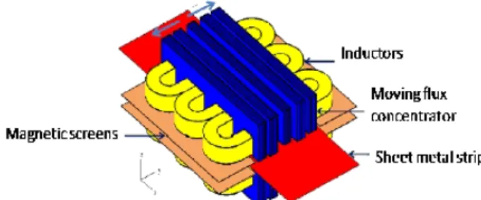
Induction heating is expanding in metal industries for applications such as melting, annealing, welding, heat treatment, drying, or merging. The heating speed, its high power density, the possibility of heating inaccessible pieces or its flexibility are all benefits. Moreover, the association to power electronic devices generally allows a precise control of the heat profile in the load. The classical solutions focus on a single inductor. Some IH generators involve multiple inductors [1][2] with moving magnetic screens and flux concentrators such as in Fig. 1. Besides, power electronics can provide a flexible solution with advantages in terms of cost and performance. Most methods for controlling the power density or the temperature in the load have been presented on single inductor heating and very few for multi-inductor systems.

Fig. 1. Transverse flux induction heating with moving parts

In [3], each inductor is powered by its own power supply constituted by a diode rectifier, a filter, an inverter

and a FPGA. A study of the temperature control is present but does not take into account the coupling between the inductors. Papers [4][5] incorporate structures of [6] to achieve control of the currents in the inductors. For this, two methods are proposed. The first [4] deals with the regulation of the amplitude and phase currents. The second [5] focuses on the real and imaginary parts of the currents. For the last one, decoupling methods are implemented. Currents are in phase and selected structures are using decoupling transformers between two inductors side by side. Inorder to keep a constant inductor current with no phase variation and no magnitude oscillation, paper [7] proposes a combination of a Pulse-Frequency-Modulation and phase-locked-loop in single phase. The analysis of the closed loop proofs the stability of the system, depending on PI regulator parameters. Comparatively, the next parts will describe our solutions, in terms of device organization and current control method. The emphasis is put on the consequences of parameter variations due to temperature rise in the disc which are considered as disturbances. Properly tuned resonant control on each of the 3 phases will reject these disturbances in order to achieve a satisfying control of the inductor currents.

II. II.MODEL OF A 3 PHASE INDUCTION HEATING SYSTEM

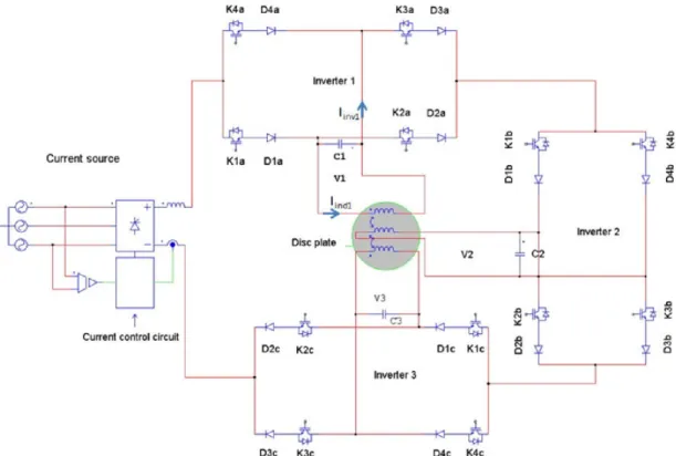
The system consists of three inductor coils (Fig.2) organized face to face in a transverse flux configuration. The work piece to be heated is a disc plate situated inside the coils. This test bench was initially developed to test different ideas such as the multi-phase supply concept and the optimization of the current references as previously described in [8][9] [10]. The whole system is supplied by 3 resonant current inverters, presented in Fig. 3. For modeling and control purposes, it can be represented by a 3 phase electrical circuit including the material to be heated where flows a current in short circuit which could be considered as the 4th_phase.

(2)

Fig. 3. Whole system schematic with inverters, controlled-current source, capacitors and coupled-inductor

After some simple calculation presented in [8][9], a matrix description of the system is given in (1) where sinusoidal currents I1, I2 and I3 feed the 3 coils. An impedance matrix [Zij] links the three inductor voltages V1, V2 and V3 to the associated inductor currents I1, I2 and I3. Different elements can be found in the real and imaginary parts of the Zij terms: self resistances and inductances of the coils, coupling terms inductors-load and mutual inductance between the inductors. = (1) = + _{² (}² _)² + + _{² (}² _)² (2) = ² ² + ( )² + + ² ² + ( )² (3)

- Mi,4: coupling terms between the inductors i and the

material to be heated (load),

- Ri, Li : self resistance and inductance for inductor i,

- R4, L4 : disc plate resistance and inductance,

- Mij : mutual inductance between inductor i and j.

As shown by (2) and (3), Zij real and imaginary parts are both nonlinear, regarding the frequency w and the temperature. Indeed, parameter R4 that models the

material resistance of the stainless steel disc is temperature dependent.Numerical simulations Flux 2Dã, Flux 3Dã or Inca 3Dã have been run to compute these parameters. But, these simulations are highly time consuming (days up to weeks in 3D configuration) and

cannot manage all the details (spiral form of the inductors for ex.). Consequently, measurements were achieved, for the real and imaginary parts of the global impedances including the coupling terms. A specific measurement procedure based on the “pseudo–energy” method from V and I measurements as previously described in [11] for a 1500Hz resonant frequency, leads to the values of the impedance matrix are given by (4) in mW.

̅ = 33.1 + 244.7i 25.9 + 43.8i25.8 + 43.6i 67.3 + 247.3i 65.9 + 113.7i21.5 + 24.3i 20.9 + 21.4i 65.2 + 111.4i 107.1 + 568.2i

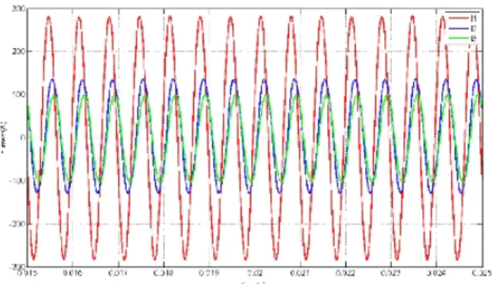
(4) In order to reach a flat temperature profile in the heated metal sheet according to the principles presented in [8][9][10], the reference currents have to be optimized through an optimization procedure. One of the best combinations of the supply currents is recalled in Table I for a required power density distribution of 10MW/m3_{in a} 0.45 radius disc made of stainless steel. The current waveforms for the inverter currents and the inductor currents are shown in Fig. 4 for phases 1 and 2 as an example with their characteristic angles for each phase i (ai, di, jij). Consequently, the current controllers will have to adjust the duty cycle ai on each phase and the phase lag jij between the inductor currents in order to follow the inductor sinusoidal reference currents.

TABLE I

BEST SETTINGS FOR A FLAT TEMPERATURE PROFILE

I1(A) I2(A) j21 _(°) I3(A) j 31 _(°)

(3)

Fig. 4. Phase 1 and 2 inverter and inductor waveforms

III. RESONANT CURRENT CONTROL

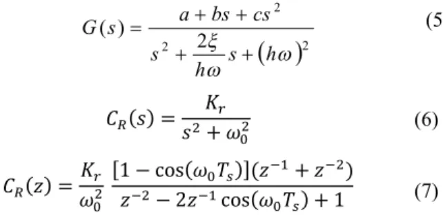
Initially proposed in [12], resonant controllers have very interesting properties when sinusoidal references of multiple frequencies have to be controlled as in [13]. Resonant controllers can achieve high performance in both multi-sinusoidal reference tracking and disturbance rejection thanks to an infinite gain at the fundamental frequency. No matrix transformation such as Park’s transformation in these controllers! Consequently, the control scheme is simpler and the computational burden is reduced. Some tuning methods can be found for such controllers, they are mainly based on Bode diagram and pole-zero map. Interesting as they may be, these methods do not take into account the time behaviour of the system since they mainly involve phase or gain margins. Moreover, they only deal with single phase systems, nothing can be found for multi-phase systems. The general form of a resonant controller can be expressed in the s-domain as in (5), where hw is the hth_{harmonic to track, x}

is a damping factor (set to zero in this case). Parameters a,

b and c must to be tuned in order to fulfil the desired

transients and stability. Besides, [14] gives a general method to tune a, b and c for robust control. It has been successfully applied in [15] for the control of a seven phase synchronous machine. The simplest resonant controller can be expressed in (6) for the continuous form and (7) for the discrete transfer function.

( )

2 2 2 2 ) ( w w x _s _h h s cs bs a s G + + + + = (5) ( ) = ₊ (6) ( ) = [1 − cos(_{− 2} _cos()]( +_{) + 1}) (7) ω0 is the frequency of the sinusoidal reference and Ts is the sampling period. Fig. 5 presents the block diagram for phase n° 1 for example, with its discrete resonant controller while Fig. 6 describes the whole 3 phase system with the coupling terms.

Fig. 5.Bloc diagram for 1 phase and resonant controller in z domain

Fig. 6 : 3 phase system with coupling and resonant controllers

zero holder 1 I1 Ts = 6KHz Ts = 6KHz Control (1-c)/wo^2z +(1-c)/wo^2z -1 -2 1-2*cz +z -1 -2 Resonant controller Ts = 6KHz 1 L11*C1.s +R11*C1.s+12 Physical process Kr 3 I3_dist1 2 I2_dist 1 I1_ref

(4)

A simple closed loop transfer function can be written in (8) without including the disturbance measurements I2 and I3 for the calculation of the control of current I1 for example in Fig.4. Nevertheless, the coupling effects will be included in the simulation model and of course in the experiments. The characteristic equation derives from (8) and leads to a stability condition using the Routh-Hurwitz criterion in s domain in (9). Conclusion is in (10).

1( ) 1 ( )

=

( ) ( ) 1+ ( ) ( )

(8) ( + )( + + 1) + = 0

(9) − < < 0 (10)

But, as stability is hard to achieve with only one tuning parameter in the z domain, a more general form of the resonant controller was used in our precedent paper [16]. The corresponding discrete transfer function was given by equation (11). Under this form, two parameters (Kr1 and Kr2) must be tuned on each phase.

( ) =

[ ( )]( ₍ ₎ )

(11)

However, stability can be achieved only with (with Kr2 equal to 0) and the search of the stable points will be easier. The corresponding discrete form of the reduced resonant controller is given by (12) .

( ) = ₍ ₎

(12)

Our precedent papers looked for the point of stability of the 3 phases separately, without taking into account the coupling effects, i.e. influence of the terms in (1). On the contrary, this paper searches the stable points of the entire system including the couplings by analyzing the norm of the poles in the discrete domain. In Fig.7 the red points are stable and the green ones are unstable. Among the stable points, the points with the smallest norm are chosen and given in Table II.

TABLE II

OPTIMAL GAINS FOR A MINIMUM POLE’S NORM

Kr1 Kr2 Kr3 Max pole’s norm

-0.06 -0.1 -0.02 0.970758

Fig. 7. Maxima of the pole norms versus the resonant controller gains

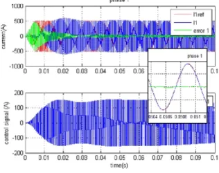
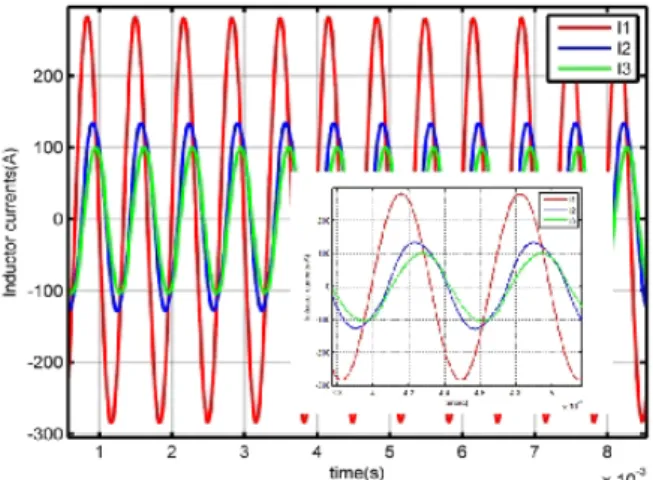
The corresponding simulated time responses are shown in Fig. 8 and 9 with very low tracking errors (zooms), small overshoot and reduced time response.

Fig. 8. reference, output current and error, control for phase 1

Fig. 9a: reference, output current and error for phase 2

Fig. 9b: reference, output current and error for phase 3

IV. ROBUSTNESS STUDY

The robustness of the system vs temperature has been simulated in the following part. Few papers deal with these considerations and even less in the case of multiphase sytems. Indeed, since the stain less steel is heated, the R4 term in terms will vary. Nevertheless, some papers such as [17] are focused on the effect of temperature dependence of magnetic properties on heating characteristics of B-H curves for a billet heater. Besides, it is claimed in [18] that temperature has no significant effect around 250°C in the field of domestic appliances. Carreterro et. al. present in [19] a comprehensive study of the temperature and frequency influence on parameters (R, L) for single phase domestic induction heating appliances. It is shown that temperature has a limited but non linear effect on the R-L parameters (max 0.2%/°C) but the system does not include the potential impact on control. This paper also points out that the metal resistivity increases with temperature and highly influences the temperature profile around 700°C. Galluin et. al. indicate in [20] that temperature dependent material properties (with Cv = Cv (T) the volume specific heat of the strip material and = l(T) its thermal conductivity)

are taken into account at each time step. Parameters are corrected according to the temperature distribution in the work piece at the previous time step but no global temperature effect is given. Consequently, it is hard to conclude especially in multi-phase systems. From our

(5)

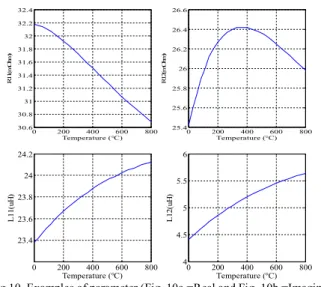
study, Fig. 10 shows the computed evolution of some Zij parameters as examples. It can be noticed that the shapes as well as the evolution rates are quite different from one to another under temperature variations in (2) and (3) through resistivity variations.

Fig 10. Examples of parameter (Fig. 10a.=Real and Fig. 10b.=Imaginary parts of Zij) variations with temperature

Since the Zij parameter variations may influence the model, their impact is checked, as depicted in Table III for the currents, in Table IV for Zij parameters and Table V where the poles-zeros variations in the closed-loop transfer functions are listed. Despite these parameter variations, the resonant controllers achieve good steady state tracking control of the inductor currents in this three-phase system, as shown in Fig. 11, 12 and 13 and in Table III for three temperatures (25°C, 200°C and 400°C).

TABLE III

SIMULATION INDUCTOR CURRENT VARIATIONS VS TEMPERATURE

25°C 200°C 400°C I1max (A) 356 356.2 357.4 I2max (A) 177.7 174.4 170 I3max (A) 130.3 127.4 125.9 phi21 (°) -41 -38.77 -39.07 phi31 (°) -60 -63.04 -67.13 TABLE IV

ZIJ PARAMETER MODEL VARIATIONS VS TEMPERATURE

25°C 200°C 400°C R11 0.0361342 0.0357361 0.0350717 R12 0.0285181 0.0292606 0.0294212 R13 0.0221604 0.0234023 0.0240771 R21 0.0285182 0.0292606 0.0294212 R22 0.0774011 0.0785965 0.0783802 R23 0.0752367 0.0767747 0.0767368 R31 0.0221604 0.0234023 0.0240771 R32 0.0752367 0.0767747 0.0767368 R33 0.1255237 0.1245204 0.1218217 X11 0.2221155 0.2248484 0.2274146 X12 0.0411916 0.0451211 0.0490916 X13 0.0194469 0.0227600 0.0262654 X21 0.0411916 0.0451211 0.0490916 X22 0.2427039 0.2527126 0.2627150 X23 0.1096059 0.1204098 0.1312485 X31 0.0194469 0.0227601 0.0262654 X32 0.1096059 0.1204098 0.1312485 X33 0.5706973 0.5854738 0.5997476 TABLE V

CLOSED-LOOP POLE AND ZERO VARIATIONS VS TEMPERATURE

Phase 1 Poles 1,2 Poles 3 , 4 Zeros

25°C 0.0445 ±0.9435i -0.0386 ± 0.9368 1; -0.9022 200°C 0.0464 ± 0.9446i -0.0405 ± 0.938 1; -0.9052 400°C 0.0486 ± 0.9459 -0.0426 ± 0.9403i 1; -0.9086

25°C -0.0711 ± 0.886 0.0767 ± 0.887 0.7613; 0.75 200°C -0.0748 ± 0.8917 0.0804 ± 0.8889 0.7699; 0.75 400°C -0.0803 ± 0.8963 0.0859 ± 0.8921i 0.7813; 0.75

25°C 0.0674 ± 0.9272 -0.0617±0.9145 1; -0.8546 200°C 0.0704±0.9272 -0.0646±0.9145 1; -0.8611 400°C 0.074±0.9316 -0.0682±0.9213 1; -0.8687

Fig. 11. Closed loop simulated inductor currents at 25°C

0 200 400 600 800 30.6 30.8 31 31.2 31.4 31.6 31.8 32 32.2 32.4 Temperature (°C) R 11 (m O hm ) 0 200 400 600 800 25.4 25.6 25.8 26 26.2 26.4 26.6 Temperature (°C) R 12 (m O hm ) 0 200 400 600 800 23.4 23.6 23.8 24 24.2 Temperature (°C) L 11 (u H ) 0 200 400 600 800 4 4.5 5 5.5 6 Temperature (°C) L 12 (u H ) 0.073 0.0735 0.074 0.0745 0.075 -300 -200 -100 0 100 200 300 Time(s) C ur re nt s in du ct or (A )a t 4 00 °C I1 I2 I3 0.0745 0.075 0.0755 0.076 -300 -200 -100 0 100 200 300 Time(s) C ur re nt s in du ct or (A )a t 2 5° C I1 I2 I3 0.075 0.0755 0.076 -300 -200 -100 0 100 200 300 Time(s) C ur re nt s in du ct or (A )a t 2 0 0° C I1 I2 I3

(6)

Table VI summarizes the simulated closed-loop currents at different operating temperatures obtained with the resonant controllers as previously tuned. It can be seen that these variations remain rather low during either transients or steady states thanks to the good performance of the resonant controllers which track the inductor currents close to their sinusoidal references. Finally, the pole norm calculation such as in Fig 5 can be launched again for several temperatures. The minimum solutions obtained in each of these different cases, leading for the minimum nom of the closed-loop poles, are all the same which put in evidence the robustness of the system.

Fig.14. Closed loop experimental evolution of the inductor current phase lags with temperature

With a precise given impedance matrix as in [4], the open-loop control signals have the right characteristics so that the inductor currents have the right amplitudes and phase lags [8]. But as the impedance matrix changes gradually according to the temperature, a predetermination strategy is impossible and the resonant controllers will help to achieve precise current control. Fig.14 shows the evolution of the phase lags of the closed loop inductor currents. The effects of the temperature rise on the current shapes remain quite low as seen in Fig. 15 and 16, where the experimental inductor currents in closed loop can be found for two temperatures 20°C and 280°C. In that case, the amplitude of the reference inductor current were reduce to ¾ of the values given in table III in order to avoid current sensor saturation (cf. table IV). Either constant amplitudes and phase lags or low distortion from one to another are achieved.

Fig.15. Closed loop experimental inductor currents at 20o_C

Fig.16. Experimental inductor currents in closed loop at 280o_C

TABLEVI

EXPERIMENTAL INDUCTOR CURRENTS VS TEMPERATURE reference 25o_{C 120}o_{C 250}o_C I1max(A) 269.3 281.4 281.4 281.4 I2max(A) 121.5 128.4 130.1 130.9 I3max(A) 98.2 100.8 101.5 102.3 Phi21(o) -49.4 -47.1 -47.3 -47.6 Phi31(o) -63.1 -61.1 -61.7 -61.8

Fig.17 shows the temperature profile around 25o_C, 120o_{C and 250}o_{C at 11 points along one radius of the} metal disc during heating. Fig.18 gives a thermal image of the metal disc at the end of the heating. It can be seen a rather homogenous temperature (except in the center of the disc of course) which confirms the good behavior of the current controllers and their ability to reach the optimal settings in order to heat the disc homogeneously.

Fig.17. Experimental temperature profiles in closed loop

Fig.18. Experimental metal disc under thermal camera at 250o_C

0 50 100 150 200 250 300 0 0, 05 _0,1 0, 15 _0,2 0, 25 _0,3 0, 35 _0,4 0, 42 5 0, 5 te m pe ra tu re ( oC) radius(m) 25C 120C 250C

(7)

Moreover, once the inductor currents are well controlled, robustness is tested by displacing the center of the metal disc by 5cm and 10cm. With 5cm displacement, the currents remain well controlled up to 278o_{C as seen in} Fig. 19, which is quite similar to Fig. 13 or 14 where the disc is in the center of the system. However, with a 10cm shift, the currents are modified at about 150o_{C in Fig. 20.}

Fig.19. Experimental inductor currents at 278o_{C and 5cm disc shift}

Fig. 20. Experimental inductor currents at 150o_{C and 10cm disc shift}

V. CONCLUSION

This paper presented a robustness study of a multi-phase induction heating system with controlled currents with the help of resonant controllers. It achieves a rather good behavior either in transients or steady states despite the coupling effects between the phases and with the load, which act as disturbances. Temperature rise has low impact on the current control and on the temperature distribution in the metal sheet. In order to reduce the temperature profile variations, temperature closed loop will be studied in future work. Additionally, the current transient control will be another interesting issue.

ACKNOWLEDGMENT

This work has been supported by French Research National Agency (ANR) through “Efficacité énergétique et réduction des émissions de CO2_{dans les systèmes} industriels” program (project ISIS n°ANR-09-EESI-004).

The authors would also like to thank Mr Philippe Texeira with at EDF R&D for his contribution and the 3rd

year ENSEEIHT students in Electrical Engineering and Control, K. Bunthern, V. Forgues-Doumenjou, A.Giani, H. T. Leluong, F. Salameh for their valuable participation during their 2013 internship.

REFERENCES

[1] T. Tudorache, V. Fireteanu, “Magneto-thermal-motion coupling in transverse flux heating”, COMPEL: The International Journal for

Computation and Mathematics in Electrical and Electronic Engineering,

vol. 27, no. 2, pp. 399-407, 2008

[2] Y. Neau, B. Paya, M. Anderhuber, F. Ducloux, J. Hellegouarch, J. Ren, “High Power transverse flux inductor for industrial heating”, in

Proc. 2003, Electromagnetic Properties of Materials Conf., pp. 570-575

[3] O. Fishman, N. Vladimir, « Gradient induction heating of a workpiece », U.S. Patent US 20090314768.

[4] H. Fujita, N. Uchida, K. Ozaki, “Zone controlled induction heating (ZCIH)–A new concept in induction heating”, in Proc. 2007

Power Conversion Conf.

[5] H.N. Pham, H. Fujita, K. Ozaki, N. Uchida, ”Dynamic analysis and control for resonant currents in a zone-control induction heating system”,

IEEE Trans. on Power Elec., vol 28, n°3, March 2013.

[6] N. Uchida, K. Kawanaka, H. Nanba, et K. Ozaki, “Induction heating method and unit”, U.S. Patent 2007012577107- June-2007.

[7] B. You; P. Xu; J.Wang; G.Zhang, “Power control of induction heating inverse power supply”, Measurement, Information and Control,

International Conference on, vol. 2, 2012 , pp. 809-812

[8] J. Egalon, S. Caux, P.Maussion, M. Souley, O. Pateau, “Multi phase system for metal disc induction heating: modeling and RMS current control”, IEEE Trans. on Industry Applications, vol. 48, no. 5, pp.1692-1699, Sept/Oct 2012

[9] M. Souley, S. Caux, O. Pateau, P. Maussion, Y. Lefèvre, “Optimization of the settings of multiphase induction heating system”, in

Proc. 2012 IAS Annual Meeting

[10] M. Souley, S. Caux, J. Egalon, O. Pateau, Y. Lefèvre, P. Maussion, “Optimization of the Settings of Multiphase Induction Heating System”,

IEEE Trans. on Industry Applications, vol., n° 99, 2013, pp 1

[11] M. Souley,A.Spagnolo, O. Pateau, B. Paya, J.C. Hapiot, P. Ladoux, P. Maussion, “Methodology to characterize the impedance matrix of multi-coil induction heating device”, in Proc. 2009 Electromagnetic

Properties of Materials Conf., pp. 201-204

[12] Y.Sato, T. Ishizuka, K. Nezu, T. Kataoka, “A New Control Strategy for Voltage-Type PWM Rectifiers to Realize Zero Steady-State Control Error in Input Current”, IEEE Trans. Ind. Appl., vol. 34, no. 3, pp. 480– 486, May/Jun. 1998.

[13] A.G. Yepes, F. D. Freijedo, O. López, J. Doval-Gandoy. “Analysis and Design of Resonant Current Controllers for Voltage-Source Converters by Means of Nyquist Diagrams and Sensitivity Function”,

IEEE Trans. on Industrial Electronics, vol. 58, no. 11, pp 5231-5250,

Nov. 2011

[14] J. Zeng, P. Degobert, D. Loriol, J.P. Hautier, "Robust design of the self-tuning resonant controller for AC current control systems", in Proc.

2005, IEEE International Industrial Technology Conf., pp. 783- 788,

[15] X. Kestelyn, Y. Crevits, E. Semail, "Auto-adaptive fault tolerant control of a seven-phase drive" in Proc. 2010, IEEE International

Industrial Electronics Symp., pp.2135-2140

[16] K.L. Nguyen, S. Caux, X. Kestelyn, O. Pateau, P. Maussion, “Resonant control of multi-phase induction heating systems”, in

Proc. 2012 IEEE Industrial Electronics Conf., pp. 3293-3298

[17] H. Kagimoto, D. Miyagi, N. Takahashi, N.Uchida, K.Kawanaka “Effect of Temperature Dependence of Magnetic Properties on Heating Characteristics of Induction Heater”, IEEE Trans. on Magnetics, vol. 46, no. 8, August 2010

[18] M. Zlobina, S. Galunin, Y. Blinov, B. Nacke, A. Nikanorov and H. Schülbe, "Numerical modeling of non-linear transverse flux heating systems", in Proc. 2003 International Scientific Colloquium, Modeling

for Electromagnetic Processing

[19] C. Carretero; J. Acero; R. Alonso; J.M. Burdio; F. Monterde; "Temperature Influence on Equivalent Impedance and Efficiency of Inductor Systems for Domestic Induction Heating Appliances”, in Proc.

2007 Applied Power Electronics Conference, pp.1233 – 1239

[20] S. Galunin, M. Blinov, Y. Kirill, “Numerical model approaches for in-line strip induction heating”, in Proc. 2009 EUROCON, pp 1607 – 1610.

(8)