A suitable parametrization to simulate slug flows with the Volume-Of-Fluid method

To link to this article: DOI:10.1016/j.crme.2012.01.003

URL :

http://dx.doi.org/10.1016/j.crme.2012.01.003

This is an author-deposited version published in:

http://oatao.univ-toulouse.fr/

Eprints ID: 8800

To cite this version:

Horgue, Pierre and Augier, Frédéric and Quintard, Michel and Prat, Marc A

suitable parametrization to simulate slug flows with the Volume-Of-Fluid

method. (2012) Comptes Rendus Mécanique, vol. 340 (n° 6). pp. 411-419. ISSN

1631-0721

O

pen

A

rchive

T

oulouse

A

rchive

O

uverte (

OATAO

)

OATAO is an open access repository that collects the work of Toulouse researchers

and makes it freely available over the web where possible.

Any correspondence concerning this service should be sent to the repository

administrator:

staff-oatao@listes.diff.inp-toulouse.fr

A suitable parametrization to simulate slug flows with the

Volume-Of-Fluid method

Pierre Horgue

a,c,∗

, Frédéric Augier

c

, Michel Quintard

a,b

, Marc Prat

a,b a_{Université de Toulouse; INPT, UPS; IMFT (Institut de Mécanique des Fluides de Toulouse), allée Camille Soula, 31400 Toulouse, France} b_{CNRS; IMFT; 31400 Toulouse, France}

c_{IFP Energies nouvelles, rond-point de l’échangeur de Solaize, BP 3, 69360 Solaize, France}

a b s t r a c t

Keywords:

Computational fluid mechanics Taylor flow

Slug flow CFD Thin film VOF method

Diffuse–interface methods, such as the Volume-Of-Fluid method, are often used to simulate complex multiphase flows even if they require significant computation time. Moreover, it can be difficult to simulate some particular two-phase flows such as slug flows with thin liquid films. Suitable parametrization is necessary to provide accuracy and computation speed. Based on a numerical study of slug flows in capillary tubes, we show that it is not trivial to optimize the parametrization of these methods. Some simulation problems described in the literature are directly related to a poor model parametrization, such as an unsuitable discretization scheme or too large time steps. The weak influence of the mesh irregularity is also highlighted. It is shown how to capture accurately thin liquid films with reasonably low computation times.

1. Introduction

When cocurrent gas and liquid flows take place within a capillary tube, there is a large number of interface configu-rations, called flow regimes or patterns in the literature, depending on the fluid properties and flow rates which can be plotted on a flow regime map (see Fig. 1 from the work of Triplett et al. [1]). One of the most common regime for the lowest liquid flow rates is the Taylor flow, also called slug flow, characterized by the presence of elongated bubbles, with diameters close to the channel tube width, separated with liquid slugs. For a higher gas flow rate, we can observe the an-nular regime characterized by the flow of a liquid film along the wall while the gas phase occupies the central void space. The common point between these flow regimes is the presence of a liquid film along the wall, which can be very thin and thus pose a serious numerical problem. Taylor flows have interesting flow characteristics such as recirculation flows in the liquid slug which improve heat and mass transfer, and, for this reason, they have been widely studied experimentally and numerically.

Previous numerical studies showed that one of the main difficulties in Taylor flow modeling concerns the simulation of the thin liquid film along the wall. Most of the previous works reported that the liquid film was not captured because the grid was not sufficiently refined. More recently, Gupta et al. [2] showed that it was possible to capture these liquid films, even thin, provided that an ultra fine mesh grid and much computation time where used. Moreover, previous works highlighted that using diffuse–interface methods can induce some numerical errors such as velocity field fluctuations around the interfaces called “spurious currents” in the literature.

In the present Note, we simulate with the Volume-Of-Fluid method (VOF), using the many possibilities offered by FLUENTTM, two cases of slug flows with the presence of a thin liquid film along the wall: the drainage of a liquid phase

*

Corresponding author at: IMFT (Institut de Mécanique des Fluides de Toulouse), allée Camille Soula, 31400 Toulouse, France.

E-mail address:horgue@imft.fr(P. Horgue).

Fig. 1. Regime flow map obtained from experiments (Triplett et al. [1]) and summarized in this figure by Gupta et al. [2].

in a vertical tube and the Taylor bubble generation in a horizontal tube. While checking the overall accuracy, a special attention is given to the liquid film modeling which have received less attention in the literature as pointed out above. Performing a parametric study on irregular meshes, VOF discretization schemes and Courant Number conditions, we first show, in the drainage case, that suitable parametrization allows to capture accurately flow properties, including the thin liquid films, while conserving small computation times and avoiding numerical errors. Applying these parameters in the Taylor bubble generation case, we show that, more generally, recommendations obtained in the previous elementary case can be extrapolated to all slug flows.

2. Numerical background

Slug flows with the presence of thin liquid films have been studied by different numerical method such as Volume-Of-Fluid (Taha and Cui [3], Akbar et al. [4], Qian and Lawal [5], Kumar et al. [6], Kashid et al. [7], Carlson et al. [8] and Gupta et al. [2]), Level-Set (Fukagata et al. [9]), Lattice-Boltzmann (Yu et al. [10]) or Phase-field (He and Kasagi [11]). The litera-ture review presented here focuses on the previous works using the same method as in this study, i.e., the VOF method. Readers interested in others methods should refer to the publications mentioned above or to the review presented in the work of Gupta et al. [2]. Taha et al. [3] simulated Taylor flows in vertical capillaries using the VOF method implemented in the FLUENTTM software. For quite large capillary numbers (higher than 0.01), and, therefore, relatively thick films, the results on bubble velocity, bubble diameter and velocity field were in good agreement with experimental data. Akbar et al. [4] demonstrated the feasibility of Taylor flow modeling with the VOF method by comparing numerical results with exper-imental data and correlations. Good agreement was found concerning bubble lengths and pressure drop for any capillary number. Regarding the liquid film thickness, more variable results were obtained depending on the simulation conditions. Qian and Lawal [5] investigated Taylor flow in a T-junction with VOF method and reported that their grid was not enough refined to capture the finest liquid films on the wall. However, numerical results on bubble length and velocity showed good agreement with literature data. Kumar et al. [6] simulated for the first time Taylor flows in curved microchannels studying the effect on the bubble lengths of different parameters such as channel diameter, curvatures, inlet conditions or fluid properties. However, none of their simulations captured the liquid film on the wall, which plays an important role in this type of flow. Kashid et al. [7] also performed numerical simulations (Level-set and VOF) on Taylor bubble generation in a Y-junction coupled with an experimental study using the micro-PIV technique. Although they simulated a bubble train, the thin liquid film observed during their experiments could not be reproduced by any of the numerical method tested. In their work, Carlson et al. [8] performed simulations on the Taylor bubbles generation in a horizontal capillary tube using two diffuse–interface methods, Level-Set and Volume-Of-Fluid. They found that the VOF method implemented in FLUENTTM

could not predict correctly the bubble generation in a slug flow.

More recently, Gupta et al. [2] performed a numerical study of Taylor flow in microchannels using the VOF method proposed in FLUENTTM. Numerical results of this study are in good agreement with the available correlations. However, they highlight the fact that an ultra fine mesh is required to capture the thin liquid film on the wall and that remain, in their simulations, some minor unphysical results such as pressure artefacts inducing spurious currents. They reduced these numerical errors by changing the way to calculate gradients in FLUENTTM (from the cell-based to the node-based methods). These spurious currents induced by the VOF formulation were studied by Harvie and Rudman [12] on a two-dimensional bubble case. They emphasize the fact that spurious currents are correlated with the implementation of the surface ten-sion effect in the VOF method, as explained in the next section concerning the method presentation. They showed that, depending on the situation, various parameters can influence the magnitude of these spurious currents such as the mesh refinement or the interface velocity. They especially highlights the fact that the spurious currents may have a big influence and can lead to unphysical behaviors of the simulations when the interface position is quasi-steady.

This literature review emphasizes the fact that many previous studies have not captured successfully the thin liquid film when simulating Taylor flows with diffuse–interface numerical methods, except using ultra fine mesh with large computa-tion time. This lack of liquid film reproduccomputa-tion can induce significant errors in the prediccomputa-tion of flow properties. Moreover, ultra fine mesh requires too large computation resources to be used at large scales.

3. Numerical method

According to the VOF model, dynamics of two immiscible fluids is governed by a single set of Navier–Stokes equations. Fluid properties (viscosity

µ

, density

ρ

) in each cell are calculated using the volume fraction, φ, which represents the proportion of each fluid in a cell, using the following relationships:

ρ

=

φ

ρ

liquid

+

(

1

−

φ)

ρ

gas (1)

µ

=

_φ

_µ

_liquid

+

₍

1

−

_φ)

_µ

_gas (2)

Like other Eulerian methods, the mesh is fixed and interfaces can be located by interpolation of the volume fraction. The Navier–Stokes system of equations contains an additional term representing the effect of surface tension (Brackbill et al. [13]):

F

=

_σ

_{(∇ ·}

n)∇φ (3)

where

σ

is the surface tension between the two fluids and n is the unit normal to the interface. This representation of the surface tension has been identified as responsible of the spurious currents along interfaces by Harvie and Rudman [12] due to the discrete representation of the domain. To illustrate their argument, they used the case of a static bubble. In a “ideal” VOF simulation, i.e., a continuous domain, the unit normal n to the interface is perfectly oriented to the center of the bubble. By solving the Navier–Stokes system, the VOF method simulates a zero velocity field with an opposite pressure gradient equivalent to the surface force. In a “real” VOF simulation, i.e., a domain discretized in cells, the volume fraction varies by step which implies that the unit normal n varies slightly and is not perfectly oriented towards the bubble center. The calculated force vector is not exact and the amplitude of the error depends on the variation ofφ within the cell. The error induced results in local recirculations of the velocity field and pressure artefacts which are relatively important in the case of static interfaces.

The volume fractionφ is transported using the VOF equation:

∂φ

∂

t

+

V

· ∇

φ =

0 (4)

where V is the fluid velocity. Usually, for unsteady-state problems, the VOF equation is solved explicitly and is decoupled from pressure and velocity computations. Variable time steps are controlled through the Courant number Co defined as follows:

Co

=

Vfluid

1

t

1

x (5)

The Courant number condition may be different for the Navier–Stokes or VOF equations. Standard FLUENTTM parameters set the Courant number condition to 0.25 for the VOF equation. In the following parametric study, we discuss the Courant number condition for the Navier–Stokes system. Since this system is solved implicitly, it represents most of the computing time and, therefore, the best gain prospect.

Another important parameter in the VOF method is the scheme used for the discretization of the convective term in Eq. (4). As the fluids are immiscible, the interface is represented by a step in φ. If we use classical “Upwind” or “2nd Order Upwind” schemes, the numerical diffusion will lead to a strong diffusion of the interface. Several strategies have been designed to overcome this numerical diffusion using specific schemes, most of them being implemented in FLUENTTM_(hence

our choice of this software for this study). The ability of a discretization scheme to transport and conserve a sharp interface is called the scheme compressibility. We described briefly below the four discretization schemes proposed by FLUENTTM, ranked from the least to the most compressive: the QUICK scheme [14], High-Resolution schemes (HRIC [15] and CICSAM [16]) and the Geometric Reconstruction scheme [17].

The QUICK scheme is based on a weighted average of 2nd order upwind and central interpolation. The central interpo-lation tends to reduce the numerical diffusion but we shall see in this paper that it remains the less compressive scheme. Based on the work of Leonard [18], high-resolution schemes have in common the alternate use of a downwind-type scheme (signal preserving and interface compression but unstable) and an upwind-type scheme (stable but diffusive). Some authors (see Ubbink and Issa [16]) reported that using a downwind-type scheme can bring numerical errors such as the alignment of the interface on the mesh grid. Improvements have been brought to high-resolution schemes by reducing the use of the downwind-type scheme depending on the interface orientation. The main difference between the HRIC and the CICSAM schemes concerns the downwind-type scheme. In the CICSAM method, the compressibility of the downwind-type scheme increases when the local Courant number decreases (due to the downwind-type scheme called HYPER-C, see Ubbink and

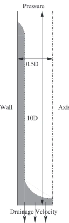
Fig. 2. Geometry and boundary condition for the drainage simulations.

Issa [16]). HRIC scheme is independent of the local Courant number and its compressibility is equivalent to the CICSAM scheme with a local Courant number condition equal to 0.5. Recommended maximum Courant number for VOF iterations is 0.25. As a result, the CICSAM scheme in our simulations is always more compressive than the HRIC scheme. A previ-ous study performed by Waclawczyk and Koronowicz [19] confirms that CICSAM preserves the shape of an interface more accurately than the HRIC scheme.

The last method called Geo-Reconstruct in FLUENTTM _{is based on the interface reconstruction concept and represents the}

most compressive solution. In a first step, the interface is transported using standard schemes which can be quite diffusive. In a second step, the numerical diffusion is canceled by interface compression using a piecewise linear interpolation (PLIC). This method is the most common method and is used in all the previous studies presented above, except in the work of Carlson et al. [8] who used the CICSAM scheme.

4. Parametric study on the drainage of a liquid phase in a vertical tube

Properties of slug flows were studied by Bretherton [20] who investigated the motion of a long bubble into a liquid-filled tube of diameter D and showed that the liquid film thickness, e, on the wall in a tube depends on the capillary number Ca (defined as the ratio of the viscous forces to interfacial tension, Ca=

µ

V/

σ

, where

µ

is the liquid viscosity, V the drainage average velocity and

σ

the two-fluid interfacial tension), according to the relationship:

2e

/

D

=

aCa2/3 (6)

valid for Ca→0 with a=1.338 for a horizontal tube. From a study of the drainage of a liquid phase in a vertical tube, Lasseux [21] extended this relationship for non-zero Bond numbers using a semi-analytical solution of the problem and then for a wide range of capillary numbers with direct numerical simulations. These simulations were performed using a Lagrangian-method, the Boundary Element Method, which discretizes explicitly the interface and follows the nodes dis-placements. This type of method has the advantage of following accurately the interface but it is quite difficult to simulate changes in the number of interfaces, and, also, it produces filled matrices in the solution procedure, which leads to heavy computations.

A vertical capillary tube of diameter 2 mm and length 10D is used for the simulations. Geometry and boundary condi-tions are reported in Fig. 2 and physical condicondi-tions are reported in Table 1. The capillary number is modified by varying the liquid phase viscosity.

Before discussing the influence of the different simulation parameters, we first perform a comparison as regards the computation of the liquid film thickness during drainage (cf. Fig. 3). VOF results fit well to the reference results obtained by Lasseux [21] with the Boundary Integral Element method, thus showing that the VOF method can simulate accurately a slug flow for a wide range of capillary numbers including thin liquid films, at least when the simulation is correctly parametrized as we shall see below. As expected, we can observe that the numerical results are in good agreement with the theory for

Table 1

Simulation conditions for the drainage of a liquid phase in a vertical tube.

Drainage velocity 0.007 m s−1 Surface tension 0.002 Liquid phase density 210 kg m−3

Bond number 1.03

Fig. 3. Dimensionless liquid film thickness as a function of capillary number during the drainage of a liquid phase in a vertical tube. Comparison between

VOF simulation and a reference solution (Lasseux [21]).

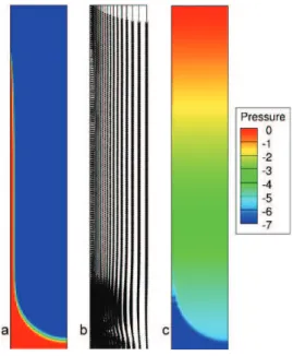
Fig. 4. Simulation of the drainage of a liquid phase (HRIC,

Co=0.25, Ca=0.005), (a) volume fraction, (b) velocity profile, (c) pressure distribution.

Fig. 5. Mesh used for VOF simulations refined from the tube wall

(left) to the center (right) with different width ratio between cells (a. 1.00 (regular), b. 1.05, c. 1.10, d. 1.20).

sufficient low capillary numbers (Ca<0.1) and diverge for higher Ca. As can be seen in Fig. 4, the velocity and pressure profiles do not present any pressure artefacts or spurious currents.

How were these results obtained? Does the choice of the various numerical parameters influence significantly the re-sults? A parametric study was done to evaluate the impact of the various choices.

The influence of the irregularity of the mesh on the liquid film thickness is first tested using four different meshes refined along the tube wall (cf. Fig. 5). Meshes have the same number of cells and, therefore, computation times for the different simulations are nearly the same. Using the HRIC scheme and a Courant number set to 0.25, our results, which are summarized in Table 2, show that irregular meshes have a small influence on the simulation results for different capillary numbers provided that the liquid film covers at least two cells. Having more than two cells in the liquid film does not seem

Table 2

Dimensionless liquid film thickness (normalized by the tube radius) for different meshes and capillary numbers (HRIC, Co=0.25) compared with the reference solution (Lasseux [21]).

Ca Lasseux [21] Regular mesh Mesh 1,05 Mesh 1,10 Mesh 1,20

0.005 0.021 0.000 0.013 0.019 0.020

0.03 0.065 0.062 0.060 0.059 0.060

0.10 0.138 0.130 0.127 0.127 0.130

Fig. 6. Simulation of drainage with spurious currents

along the meniscus curvature (HRIC, Co=1.00, Ca= 0.03), (a) volume fraction, (b) velocity profile, (c) pres-sure distribution.

Fig. 7. Simulation of drainage with spurious currents

along the liquid film (CICSAM, Co=0.05, Ca=0.03), (a) volume fraction, (b) velocity profile, (c) pressure dis-tribution.

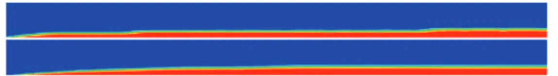
Fig. 8. Alignment of the interface on the mesh when VOF scheme is too compressive, for example with the Geo-Reconstruct scheme (top) compared with

the HRIC scheme (bottom).

to lead to a better accuracy. Our results show that it is possible to capture accurately thin films (less than 1% of the radius) while conserving small computation time by locally refining the mesh.

In a second phase, a parametric study on the VOF schemes and the Courant number was performed. In the case of a poor model parametrization, spurious currents (in parallel with pressure artefact) can occur around interfaces, which was previously observed by Gupta et al. [2] and Harvie and Rudman [12]. For all the tested VOF schemes, we observed that, when Co>0.25, these spurious currents occur around the meniscus curvature and increase with the Courant number Co (an example is shown in Fig. 6). These pressure artefacts and spurious currents also appear at the triple point (intersection of the interface with the wall) and move along the liquid film (cf. Fig. 7) when the liquid film becomes thin (2e<0.10D) for the two most compressive methods, Geo-Reconstruct and CICSAM. As in the study of Harvie and Rudman [12], we observe, in this area, a curvature of the interface on a small number of cells. We can presume that the compressibility of these two schemes, which reduces the thickness of the interface, increases the intensity of the interfacial force on a small number of cells (i.e., the ∇φ term in the Navier–Stokes equations), and, therefore, the local spurious effects. Moreover, the link of these spurious effects to interface compression can be directly emphasized using the CICSAM scheme properties. By reducing the Courant number for the same simulations, we increase the compressibility of the CICSAM scheme (see Ubbink and Issa [16]) and we can observe that it simultaneously increases the amplitude of the spurious currents generated. The interface compression can also lead to the alignment of the interface on the mesh grid that was previously described by Ubbink and Issa [16]. Then, the interface thickens by step along the tube wall as it can be seen in Fig. 8.

We also performed simulations using different discretization schemes which are available in FluentTM (“1st Order Up-wind”, “2nd Order Upwind” and “3rd Order MUSCL”). As the influence of these schemes was very weak compared to the previously cited parameters, we did not incorporate these parameters to this parametric study.

Table 3

Interface thickness at the front/film (in number of cells).

Courant number 0.05 0.25 0.50 1.00

QUICK 6.86/3.40 5.76/3.33 9.68/3.40 14.02/3.73

HRIC 4.32/3.33 3.34/2.80 3.96/2.73 4.58/2.80

CICSAM 2.56/1.93 2.61/2.73 2.34/2.47 2.54/2.60

Geo-Reconstruct 1.98/1.92 2.05/1.93 1.93/1.92 1.86/1.94

Fig. 9. A comparison of the interface dissipation from the less to the most compressive scheme (Co=0.25, Ca=0.03), (a) QUICK, (b) HRIC, (c) CICSAM, (d) Geo-Reconstruct.

Fig. 10. Geometry and boundary conditions for the Taylor bubbles simulations.

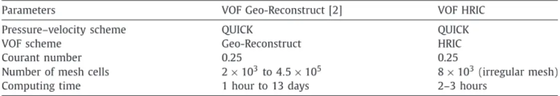
Table 4

Parameters of the two numerical simulations studied.

Parameters VOF Geo-Reconstruct [2] VOF HRIC

Pressure–velocity scheme QUICK QUICK

VOF scheme Geo-Reconstruct HRIC

Courant number 0.25 0.25

Number of mesh cells 2×103_{to 4.5×10}5 _8×103_{(irregular mesh)}

Computing time 1 hour to 13 days 2–3 hours

The interface thickness (in numbers of cells) at the front and along the film for different schemes and Courant numbers are displayed in Table 3. The CICSAM and Geo-Reconstruct methods conserve sharp interfaces but, as seen before, there is no valid Courant number to obtain consistent velocity and pressure fields. The QUICK and HRIC schemes are both able to simulate correctly the properties (velocity profile, liquid film thickness) of the slug flow. However, as shown in Fig. 9, the QUICK scheme is more diffusive that the HRIC scheme and it can lead to interface disappearance when the flow becomes more complex.

As a conclusion to this parametric study, the HRIC scheme, with Co=0.25, seems to be the optimal combination of parameters to simulate accurately slug flows with thin liquid films while avoiding the numerical errors described above. This optimal combination of parameters have been used to perform the comparison related in Fig. 3.

So far, we have studied a simple flow geometry, with the emphasis on the film accurate simulation. The existence of a well established reference helped us to draw practical conclusions in terms of suitable numerical parameters. What happens in the case of more complex situations, for which there is a little a priori knowledge of the obtained configuration?

5. Validation case: Taylor bubble generation

Taylor bubble generation in a horizontal capillary tube is a good test case since films and meniscii are present in an unsteady-state flow. Like in the study of Gupta et al. [2], we inject air and water (superficial velocities are respectively 0.245 and 0.255 m/s) in an initially liquid filled microchannel with diameter, D, of 0.5 mm and length of 10D as depicted on Fig. 10. The conditions of the simulations, summarized in Table 4, are the same as Gupta et al. [2] except for the VOF scheme and the mesh grid used. As the expected dimensionless film thickness is around 0.02D, we use a sufficiently refined irregular mesh with a width ratio of 1.10, i.e., between 2 and 3 cells included in the liquid film. Plots of the liquid volume fraction during the simulation at different times can be seen in Fig. 11 and results of simulations are reported in Table 5.

Concerning the film thickness, bubble velocity and gas hold-up, our simulations fit pretty well with reference values. We can note that bubble and slug lengths are quite different between the two simulations even if the gas hold-up is nearly the

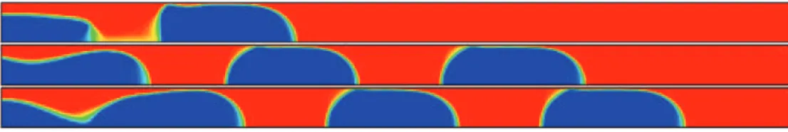
Fig. 11. VOF simulations of the process of bubble generation in a microchannel using the HRIC scheme at different times (3.6 ms, 7.0 ms and 8.5 ms).

Table 5

Comparisons of numerical results (with reference values).

Flow properties VOF Geo-Reconstruct [2] VOF HRIC

Film thickness (µm) 12 (11) 12 (11)

Bubble velocity (m s−1_{) 0.55 (0.54) 0.56 (0.54)}

Bubble length 2.0D 1.62D

Slug length 1.3D 1.07D

Gas hold-up 0.455 (0.41) 0.414 (0.41)

Pressure drop (Pa m−1_{) 77 700 (94 400) 137 000 (112 000)}

Fig. 12. Volume fraction and Pressure distribution around a typical Taylor bubble simulated with the VOF method (HRIC, Co=0.25).

same (bubble length depending on the inlet conditions). To calculate a reference value for the pressure drop, we use the correlation for the friction factor proposed by Kreutzer et al. [22]:

f

=

16 Re

·

1

+

0

.

071 Ls

µ

_Re Ca

¶

0.33

¸

(7) where Re is the Reynolds number and Ls=Lslug/D is the dimensionless slug length. Pressure drop can be calculated by the

following equation:

1

P L

=

f

µ

₁ 2

ρ

LU 2

¶

4 D

β

L (8)

where βL is the liquid hold up and U the sum of gas and liquid superficial velocities. Difference between correlated and computed pressure drops is around 20% for the two types of simulations. As can be seen from Fig. 12, the pressure field simulated with the HRIC scheme does not present any artefact in the tail or the head of the Taylor bubble. We can note that the creation of bubbles induces a small diffusion at the tail of the bubble (cf. Fig. 11 and Fig. 12) contrary to the Geo-Reconstruct method which always conserves a sharp interface. This interface diffusion gradually disappears thanks to the scheme compressibility. In terms of computation time (cf. Table 4), capturing the liquid film with the Geo-Reconstruct method requires ultra fine mesh and several days of calculations [2]. Using a suitable irregular mesh with the HRIC scheme reduces the computation time to a couple of hours for the same physical conditions.

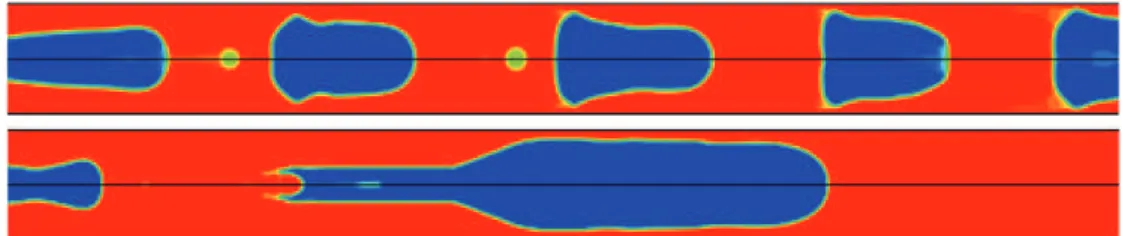
As a test, we also performed a qualitative comparison by changing the simulation conditions. Carlson et al. [8], reported that the VOF method (with the CICSAM scheme) failed to simulate the generation of a regular bubble train. Similar sim-ulations were carried out in the same conditions using the HRIC and CICSAM schemes. Similar results as in the work of Carlson et al. [8] were observed concerning the CICSAM scheme, i.e., the random generation of bubble of different sizes, while the use of the HRIC scheme allows simulating correctly the flow phenomenology (see Fig. 13). However, we can also see in Fig. 13 that the interface dissipation becomes more important, which suggests a limit to the HRIC scheme.

6. Conclusions

We emphasized in this Note that simulating slug flows with the VOF method needs suitable parameterization to provide computation speed and accuracy. We mainly focus on capturing thin liquid films on the walls which is the most difficult

Fig. 13. A qualitative comparison of VOF simulations of bubble generation using HRIC scheme (top) and CICSAM scheme (bottom).

aspect of the problem. We first validated quantitatively VOF simulations in the case of the classical Bretherton dynamic film and conclusions provided by the parametric study highlight some aspects which must be considered to simulate slug flows with the VOF method:

– irregular meshes have a small influence on computed results provided that the liquid film is covered by at least two cells, which allows refining locally the mesh and gain much computation time;

– Courant number must be chosen sufficiently small to avoid pressure artefacts and spurious currents around interfaces; – using the most compressive scheme induces numerical errors and does not represent the best choice for simulating

thin liquid films; less compressive schemes allow using coarser meshes while maintaining good accuracy and avoiding the different numerical errors described above.

In the specific case of slug flows in capillaries, the HRIC scheme with a Courant number of 0.25 and an irregular mesh depending on the expected liquid film is the best suited to simulate accurately the properties of slug flows. However, the process of bubble creation induces interface dissipation which is obviously more important for the least compressive schemes. This observation suggests that the most compressive schemes will be probably more suited to simulate flow regimes with many interface changes such as the bubbly flow.

References

[1] K. Triplett, S. Ghiaasiaan, S. Abdel-Khalik, D. Sadowski, Gas-liquid two-phase flow in microchannels, Part 1: Two-phase flow patterns, Int. J. of Multi-phase Flow 25 (3) (1999) 377–394.

[2] R. Gupta, D. Fletcher, B. Haynes, On the cfd modelling of Taylor flow in microchannels, Chem. Eng. Sci. 64 (2009) 2941–2950. [3] T. Taha, Z.F. Cui, Hydrodynamics of slug flows inside capillaries, Chem. Eng. Sci. 59 (6) (2004) 1181–1190.

[4] M. Akbar, S.M. Ghiaasiaan, Simulation of Taylor flow in capillaries based on the volume-of-fluid technique, Ind. Eng. Chem. Res. 45 (2006) 5396–5403. [5] D. Qian, A. Lawal, Numerical study on gas and liquid slgus for Taylor flow in a t-junction microchannel, Chem. Eng. Sci. 61 (23) (2006) 7609–7625. [6] V. Kumar, S. Vashisth, Y. Hoarau, K. Nigam, Slug flow in curved microreactors: Hydrodynamic study, Chem. Eng. Sci. 62 (2007) 7494–7504.

[7] M. Kashid, D. Rivas, D. Agar, D. Turek, On the hydrodynamics of liquid–liquid slug flow capillary microreactors, Asia–Pac. J. Chem. Eng. 3 (2) (2008) 151–160.

[8] A. Carlson, P. Kudinov, C. Narayanan, Prediction of two-phase flow in small tubes: a systematic comparison of state-of-art cmfd codes, in: 5th European Thermal-Sciences Conference, 2008.

[9] K. Fukagata, N. Kasagi, P. Ua-arayaporn, T. Himeno, Numerical simulation of gas–liquid two-phase flow and convective heat transfer in a micro tube, Int. J. Heat Fluid Flow 28 (1) (2007) 72–82.

[10] Z. Yu, O. Hemminger, L.-S. Fans, Experiment and lattice Boltzmann simulation of two-phase gas–liquid flows in microchannels, Chem. Eng. Sci. 62 (2007) 7172–7183.

[11] Q. He, N. Kasagi, Phase-field simulation of small capillary-number two-phase flow in a microtube, Flow Dynamics Research 40 (7–8) (2008) 497–509. [12] D. Harvie, M. Rudman, An analysis of parasitic current generation in volume of fluid simulations, Appl. Math. Model. 30 (10) (2006) 1056–1066. [13] J.U. Brackbill, D. Kothe, C. Zemach, A continuum method for modelling surface tension, J. Comput. Phys. 100 (1992) 335–354.

[14] B. Leonard, S. Mokhtari, ULTRA-SHARP nonoscillatory convection schemes of high-speed steady multidimensional flow, in: NASA TM 1-2568 (ICOMP-90-12), NASA Lewis Research Center, 1990.

[15] S. Muzaferija, M. Peric, P. Sames, T. Schellin, A two-fluid Navier–Stokes solver to simulate water entry, in: Proc. 22nd Symposium on Naval Hydrody-namics, 1998.

[16] O. Ubbink, R.I. Issa, A method for capturing sharp fluid interfaces on arbitrary meshes, J. Comput. Phys. 153 (1999) 26–50.

[17] D. Youngs, Time-dependent multi-material flow with large distortion, in: K.W. Morton, M.J. Baines (Eds.), Numerical Methods for Fluid Dynamics, Academic Press, London.

[18] B.P. Leonard, The ultimate conservative difference scheme applied to unsteady one-dimensional advection, Comput. Meth. Appl. Mech. Eng. 88 (1991) 17–74.

[19] T. Waclawczyk, T. Koronowicz, Comparison of CICSAM and HRIC high-resolution schemes for interface capturing, J. Theor. Appl. Mech. 46 (2008) 325– 345.

[20] F. Bretherton, The motion of long bubbles in tubes, J. Fluid. Mech. 10 (1961) 166–188.

[21] D. Lasseux, Caractérisation expérimentale, analytique et numérique d’un film dynamique lors du drainage d’un capillaire, Ph.D. thesis, Université de Bordeaux I, 1990.

[22] M. Kreutzer, F. Kapteijn, J. Moulijn, C. Kleinj, J. Heiszwolf, Inertial and interfacial effects on pressure drop of Taylor flow in capillaries, AICHE J. 51 (9) (2005) 2428–2440.