O
pen
A
rchive
T
OULOUSE
A
rchive
O
uverte (
OATAO
)
OATAO is an open access repository that collects the work of Toulouse researchers and
makes it freely available over the web where possible.
This is an author-deposited version published in :
http://oatao.univ-toulouse.fr/
Eprints ID : 6276
To link to this article :
URL : http://ieeexplore.ieee.org/xpl/articleDetails.jsp?arnumber=6168272
To cite this version : Pereyra, Marcelo and Dobigeon, Nicolas and
Batatia, Hadj and Tourneret, Jean-Yves Segmentation of skin
lesions in 2D and 3D ultrasound images using a spatially coherent
generalized Rayleigh mixture model. (2012) IEEE Transactions on
Medical Imaging, vol. 31 (n° 8). pp. 1509-1520. ISSN 0278-0062
Any correspondence concerning this service should be sent to the repository
administrator:
[email protected]
㩷Segmentation of Skin Lesions in 2-D and 3-D
Ultrasound Images Using a Spatially Coherent
Generalized Rayleigh Mixture Model
Marcelo Pereyra*, Nicolas Dobigeon, Hadj Batatia, and Jean-Yves Tourneret
Abstract—This paper addresses the problem of jointly
es-timating the statistical distribution and segmenting lesions in multiple-tissue high-frequency skin ultrasound images. The distribution of multiple-tissue images is modeled as a spatially coherent Þnite mixture of heavy-tailed Rayleigh distributions. Spatial coherence inherent to biological tissues is modeled by enforcing local dependence between the mixture components. An original Bayesian algorithm combined with a Markov chain Monte Carlo method is then proposed to jointly estimate the mixture parameters and a label-vector associating each voxel to a tissue. More precisely, a hybrid Metropolis-within-Gibbs sam-pler is used to draw samples that are asymptotically distributed according to the posterior distribution of the Bayesian model. The Bayesian estimators of the model parameters are then computed from the generated samples. Simulation results are conducted on synthetic data to illustrate the performance of the proposed estimation strategy. The method is then successfully applied to the segmentation of in vivo skin tumors in high-frequency 2-D and 3-D ultrasound images.
Index Terms—Bayesian estimation, Gibbs sampler, heavy-tailed
Rayleigh distribution, mixture model, Potts–Markov Þeld.
I. INTRODUCTION
U
LTRASOUND imaging is a longstanding medical imaging modality with important applications in di-agnosis, preventive examinations, therapy and image-guided surgery. In dermatologic oncology, diagnosis relies mainly on surface indicators such as color, shape, and texture whereas the two more reliable measures are the depth of the lesion and the number of skin layers that have been invaded. Currently, these can only be evaluated after excision. Recent advances in high-frequency transducers and 3-D probes have opened new opportunities to perform noninvasive diagnostics using ultra-sound images. However, changing dermatological practices requires developing robust segmentation algorithms. Despite the extensive literature on the subject, accurate segmentation*M. Pereyra is with the University of Toulouse, IRIT/INP-ENSEEIHT, 31071 Toulouse Cedex 7, France (e-mail: [email protected]).
N. Dobigeon, H. Batatia, and J.-Y. Tourneret are with the Univer-sity of Toulouse, IRIT/INP-ENSEEIHT, 31071 Toulouse Cedex 7, France (e-mail: [email protected]; [email protected]; [email protected]).
of ultrasound images is still a challenging task and a focus of considerable research efforts. Current segmentation tech-niques are extremely application-speciÞc, developed mainly for echocardiography followed by transrectal prostate examination (TRUS), kidney, breast cancer and (intra) vascular diseases (IVUS) [3]. A survey of the state-of-the-art methods up to 2006 is presented in [3].
Segmentation in echocardiography, TRUS and IVUS is mainly concerned with the detection and tracking of organ boundaries. Lesion delimitation is signiÞcantly different and more challenging. On one hand, unlike organs, lesions ex-hibit soft or “fuzzy” edges that are difÞcult to capture with boundary detection techniques. On the other, their echogenic and statistical characteristics are visibly different from those of their surrounding tissues. This fact has motivated the devel-opment of region-based segmentation techniques as opposed to boundary-based methods, which are still an active research subject in other medical ultrasound domains [4]–[6]. Similarly, lesions do not have anatomically predeÞned shapes as is the case for organs and are unlikely to beneÞt in the near future from recent works on anatomical or learned statistical shape priors [7]–[9]. This might change with the improvement of geometric tumor growth models derived from computational biology [10]. Early lesion segmentation methods have focused mainly on thresholding [11], [12] and were superseded by texture-based techniques. Madabhushi et al. derived an active contour based on texture and boundary features [13]. Huang
et al. proposed a texture segmentation technique based on a
neural network and a watershed algorithm [14]. In addition, Gaussian mixture models coupled with Markov random Þelds were proposed to segment lesions based on their region sta-tistics [15], [16]. Moreover, since the important work of Dias
et al. [17], Rayleigh mixtures have become a powerful model
for region-based ultrasound image segmentation. The use of Rayleigh instead of Gaussian distributions is strongly justiÞed by the physics of the image formation process that generates B-mode ultrasound images [18]. Based on the assumption that each biological tissue has its proper Rayleigh statistics, tissue segmentation is achieved by separating the mixture compo-nents. This is achieved by Þnding the maximum-likelihood (ML) or maximum-a-posteriori (MAP) estimators of the lesion contours. The optimization problem stemming from the ML and MAP estimators was solved in [17] using an interactive dynamic programming algorithm that jointly estimated the MAP contour and the mixture parameters. The authors per-formed several experiments on real echocardiography images and showed that the proposed method accurately segments heart walls.
With the development of deformable models, Brusseau et al. proposed a statistical parametric active contour (AC) [19]. A parametric AC is a regularized curve deÞned by a set of points in the image domain that can be moved to maximize the seg-mentation posterior [20]. In the work of Brusseau et al., the two-mixture components were separated using a statistical re-gion AC which iteratively estimated the Rayleigh parameter of each component and evolved to optimize the segmentation. Also, given that convergence to a global optimum is not guar-anteed, the authors proposed an ad-hoc automatic initialization technique. This method was further improved by Cardinal et al. [21] who substituted the parametric AC by an edge-based level set (LS) derived from the original work of Osher and Sethian [22]. A second modiÞcation was the introduction of an expecta-tion-maximization (EM) algorithm to estimate the mixture pa-rameters during initialization, thus removing the need to esti-mating them iteratively. The authors reported that the Rayleigh mixture LS method outperforms classical gradient-based LS at intravascular image segmentation. In addition, Saroul et al. re-cently applied the Rayleigh mixture model to prostate segmen-tation in transrectal ultrasound images [23]. In this case, the LS was replaced by a deformable model based on a super ellipse whose evolution was computed using a variational algorithm. The authors showed that the regularization introduced by this deformable model could compensate partial occlusion.
Rayleigh-mixture models were extended to tissues with gen-eralized Rayleigh statistics by Destrempes et al. [24], who pro-posed a carotid artery segmentation method based on a Nak-agami mixture and a deformable model. As in [21], the estima-tion of the mixture parameters was achieved using an EM algo-rithm under the assumption that observations are independent. The evolution of the deformable model was computed using exploration/selection, a stochastic optimization algorithm that converges to the global optimum. However, since the mixture parameters are estimated with an EM algorithm, overall global convergence is not guaranteed. One other important contribu-tion is the Rayleigh region-based LS method presented in [25], that adapted the fundamental work of Chan and Vese [26] on ACs without edges to ultrasound images with Rayleigh statis-tics. These region-based LS should be very appropriate for ul-trasound images of lesions as they are able to segment objects with smooth edges under poor signal-to-noise ratio conditions. This work was recently generalized to all the distributions from the exponential family (i.e., Gamma, Rayleigh, Poisson, etc.) in [27]. However, these methods have not yet been applied to le-sion segmentation in ultrasound images.
This paper addresses the problem of jointly estimating the statistical distribution and segmenting lesions in multiple-tissue 2-D and 3-D high-frequency skin ultrasound images. To our knowledge this is the Þrst ultrasound image segmentation method speciÞc to skin lesions. We propose to model mul-tiple-tissue images using a heavy-tailed Rayleigh mixture, a model that has been inspired by the single-tissue model studied in [28]. The proposed mixture model is equipped with a Markov random Þeld (MRF) that takes into account the spatial correla-tion inherent to biological tissues. Note that Potts Markov Þelds are particularly well suited for label-based segmentation as explained in [29] and further studied in [30]–[33]. Potts Markov models enhance segmentation because of their ability to capture the spatial correlation that exists between neighbor class labels
[30]. This correlation arises naturally from the spatial organi-zation of biological tissues and is particularly important in skin because of its layered structure. Finally, while the Potts prior is an effective means to introduce spatial correlation between the class labels, it is interesting to mention that other more complex models could have been used instead. In particular, Marroquin
et al. [34] have shown that better segmentation results may be
obtained by using a two-layer hidden Þeld, where hidden labels are assumed to be independent and correlation is introduced at a deeper layer by a vectorial Markov Þeld. Similarly, Woolrich
et al. [35] have proposed to approximate the Potts Þeld by
modeling mixture weights with a Gauss–Markov random Þeld. However, these alternative models are not well adapted for 3-D images because they require signiÞcantly more computation complexity and memory resources than the Potts model. These overheads result from the fact that they introduce
and hidden variables, respectively, against only for the Potts model ( being the number of voxels and the number of classes). In addition, the segmentation problem is solved using a stochastic optimization algorithm with guaranteed global convergence, removing the need for an initial contour or supervised training. The paper is organized as follows. The statistical model used for an ultrasound image voxel is intro-duced in Section II. Section III introduces the Bayesian model used for the segmentation of ultrasound images. An hybrid Gibbs sampler generating samples asymptotically distributed according to the posterior distribution of this Bayesian model is described in Section IV. Experiments on synthetic and real data are presented in Section V. Conclusions are Þnally reported in Section VI.
II. PROBLEMSTATEMENT
This section describes the mixture model used for ultrasound image voxels. Let denote an observation, or voxel, in an envelope (B-mode) ultrasound image
without logarithmic compression. We assume that is deÞned by means of the widely accepted point scattering model [36]
(1) where is the total number of punctual scatterers,
denotes the analytic extension of the interrogating pulse , is the cross-section of the th scatterer, is the time of arrival of the th backscattered wave and is the sampling time associated with . Recent works on scattering in biological tissues have established that , as deÞned above, converges in distribution towards an -Rayleigh distribution as
increases [28]
(2) where denotes convergence in distribution, the parame-ters and are the characteristic index and spread associated with the th voxel.
This paper considers the case where the ultrasound image is made up by multiple biological tissues with high scatter density (i.e., ), each with its own echogenicity and therefore its proper speckle statistics. In view of this spatial conÞguration,
we propose to model by an -Rayleigh stationary process with piecewise constant parameters. More precisely, we assume that there is a set of stationary classes such that
(3) where and are the parameters associated with the class (i.e., the th biological tissue). As a consequence, it is possible to express the distribution of by means of the following mix-ture of -Rayleigh distributions
(4) where is the number of classes and represents the relative weight (or proportion) of the th class with . Lastly, to take into account the spatial coherence inherent to biological tissues we will consider that the class of a given voxel depends on those of its neighbors.
It should be noted that the proposed -Rayleigh mixture model is closely related to two other mixture models. On the one hand it generalizes the Rayleigh mixture model, which has been extensively applied to ultrasound image modeling. On the other, it can be shown that before being transformed by acquisi-tion and demodulaacquisi-tion, radio-frequency ultrasound signals are distributed according to a symmetric -stable distribution [28]. Hence, the proposed -Rayleigh mixture model can be inter-preted as a transformation of the symmetric -stable mixture model studied in [37]. In addition, it is interesting to mention that the -Rayleigh distribution has been used successfully for SAR images in [38] and [39]. The methods proposed in [38] and [39] have been recently applied to characterize tissues in annotated ultrasound images [28]. This paper extends those methods by including in the estimation problem the identiÞca-tion of regions in the image with similar -Rayleigh parameters (each region being associated with a different tissue). This is achieved by proposing a novel Bayesian estimation algorithm based on the -Rayleigh mixture model (4) coupled with an MRF prior that captures the spatial coherence inherent to bio-logical tissues. Finally, akin to [19], [21], [24], [25], note that the model (4) uses a simpliÞed image representation based on regions and does not describe the boundaries between tissues explicitly.
The following section addresses the problem of estimating the parameters of the spatially coherent -Rayleigh mixture model introduced in (4) and performing the segmentation of ul-trasound images.
III. BAYESIANMODEL
A label vector is introduced to map ob-servations to classes (i.e., if and only if ). This label vector will allow each image obser-vation to be characterized and different kinds of tissues to be discriminated. Note that the weights are directly related to the labels through the probabilities for
. Consequently, the unknown parameter vector for the mixture (4) can be deÞned as where with
and . This section
Fig. 1. Four-pixel (left) and eight-pixel (right) neighborhood structures. The pixel considered appears as a void red circle whereas its neighbors are depicted in full black and blue.
studies a Bayesian model associated with . This model re-quires deÞning the likelihood and the priors for the unknown parameters.
A. Likelihood
Assuming that the observations are independent and using the mixture model (4), the likelihood of the proposed Bayesian model can be written as
(5) where denotes the subset of indexes
that verify and
(6) is the probability density function (pdf) of an -Rayleigh dis-tribution with parameters and and is the zeroth-order Bessel function of the Þrst kind.
B. Parameter Priors
1) Labels: It is natural to consider that there is some
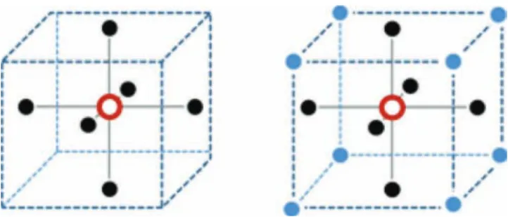
cor-relation between the probabilities of a given voxel and those of its neighbors. Since the seminal work of Geman [40], MRFs have become very popular to model neighbor cor-relation in images. MRFs assume that the distribution of a pixel conditionally to all other pixels of the image equals the distribu-tion of this pixel condidistribu-tionally to its neighbors. Consequently, it is important to properly deÞne the neighborhood structure. The neighborhood relation between two pixels (or voxels) and has to be symmetric: if is a neighbor of then is also a neighbor of . There are several neighborhood structures that have been used in the literature. In the bidimensional case, neighborhoods deÞned by the four or eight nearest voxels rep-resented in Fig. 1 are the most commonly used. Similarly, in the tridimensional case the most frequently used neighborhoods are deÞned by the six or fourteen nearest voxels represented in Fig. 2. In the rest of this paper four-pixel neighborhoods will be considered for 2-D images and six-voxel neighborhoods for 3-D images. Therefore, the associated set of neighbors, or cliques, can only have vertical, horizontal and depth conÞgurations (see [40] and [41] for more details).
Once the neighborhood structure has been established, the MRF can be deÞned. Let denote the random vari-able indicating the class of the th image voxel. In the case
Fig. 2. Six-voxel (left) and fourteen-voxel (right) neighborhood structures. The voxel considered appears as a void red circle whereas its neighbors are depicted in full black and blue.
of classes, the random variables take their values in the Þnite set . The whole set of random variables forms a random Þeld. An MRF is then deÞned when the conditional distribution of given the other pixels only depends on its neighbors , i.e.,
(7) where contains the neighbors of according to the neigh-borhood structure considered.
In this study, we will Þrst consider 2-D and 3-D Potts Markov Þelds as prior distributions for . More precisely, 2-D MRFs are considered for single-slice (2-D) ultrasound images whereas 3-D MRFs are used for multiple-slice (3-D) images. In light of the Hammersley–Clifford theorem, the corresponding prior for
can be expressed as follows:
(8)
where is the granularity coefÞcient, is the normalizing constant or partition function [42] and is the Kronecker function. The hyperparameter tunes the degree of homo-geneity of each region in the image. A small value of induces a noisy image with a large number of regions, contrary to a large value of that leads to few and large homogeneous regions. In this work, the granularity coefÞcient will be Þxed a priori. However, it is interesting to mention that the estimation of has been receiving a lot of attention in the literature [33], [43]–[46]. Estimating the granularity coefÞcient using one of these methods is clearly an interesting problem that will be investigated in future work. Finally, it is interesting to note that despite not knowing , drawing labels
from the distribution (8) can be easily achieved by using a Gibbs sampler [47].
2) -Rayleigh Parameters: The prior for each characteristic
index is a uniform distribution on
(9) This choice is motivated by the fact that the only information available a priori about this parameter, is that it can take values in the interval .
Fig. 3. DAG for the -Rayleigh mixture model (the Þxed nonrandom hyper-parameters appear in dashed boxes).
The prior for each spread parameter is an inverse gamma distribution with hyperparameters and
(10) This choice is motivated by the fact that the inverse gamma dis-tribution allows either very vague or more speciÞc prior infor-mation to be incorporated depending on the choice of the hy-perparameters and ( will be used in our experiments corresponding to a vague prior distribution).
Assuming a priori independence between the parameters and , the prior for is
(11) We will also assume that the -Rayleigh parameters are inde-pendent from the labels associated with the image voxels. Thus the joint prior for the unknown parameters can be ex-pressed as
(12) where has been deÞned in (8) and in (11).
Fig. 3 presents the proposed Bayesian model as a directed acyclic graph (DAG) summarizing the relationships between the different parameters and hyperparameters.
C. Posterior Distribution of
Using Bayes theorem, the posterior distribution of can be expressed as follows:
(13) where means “proportional to” and the likelihood
and the joint prior have been deÞned in (5) and (12). Unfortunately, the posterior distribution (13) is too complex to derive closed form expressions for the minimum mean square error (MMSE) or MAP estimators of the unknown parameters , and 1. One can think of using the EM algorithm [48] that has received much attention for mixture problems (see [21] and [24] for applications to ultrasound images). However, EM algorithms have many known shortcomings. For instance, they
1Note that involves the potential of a Potts Markov Þeld and its
in-tractable partition function and that is the product of indeÞ-nite integrals
suffer from convergence to local maxima or saddle points of
the log-likelihood function and sensitivity to starting values
[49, p. 259]. Note that analyzing the concavity properties of the logarithm of (5) is not easy because the -Rayleigh distribution does not belong to the exponential family. An interesting alternative is to use a Markov Chain Monte Carlo (MCMC) method generating samples that are asymptotically distributed according to the target distribution (13) [47]. The generated samples are then used to approximate the Bayesian estima-tors. This strategy has been used successfully in many image processing applications [50]–[54]. One sampling technique allowing the parameters of ultrasound images to be estimated is studied in the next section.
IV. HYBRIDGIBBSSAMPLER
This section studies a hybrid Metropolis-within-Gibbs sam-pler for generating samples that are asymptotically distributed according to (13). The histogram of the generated samples is guaranteed to converge to the posterior (13) [47, p. 269]. One of the most popular methods for generating samples distributed according to a distribution whose pdf or probability masses are known up to a multiplicative constant is the Gibbs sampler. The conventional Gibbs sampler draws samples according to the conditional distributions associated with the distribution of in-terest [here the posterior (13)]. When a conditional distribution cannot be sampled easily, one can resort to a Metropolis–Hast-ings (MH) move, which generates samples according to an ap-propriate proposal and accept or reject these generated sam-ples with a given probability. The resulting sampler is referred to as Metropolis-within-Gibbs sampler (see [47] for more de-tails about MCMC methods). The sampler investigated in this section is based on the conditional distributions , , and that are described in the next para-graphs (see also [55, Algor. 1]).
A. Conditional Probability
The label vector can be updated coordinate-by-coordinate using Gibbs moves. More precisely, the conditional probabili-ties can be computed using Bayes’ rule
(14) where (it is recalled that is the number of classes) and where is the vector whose th element has been removed. The probability (14) is proportional to
(15)
where has been deÞned in (6) and is evaluated using the approximations presented in paragraph Section IV-D. Once all the quantities , , have
been computed, they are normalized to obtain the posterior
probabilities as follows:
(16)
Note that the posterior probabilities of the label vector in (15) and (16) deÞne an MRF. Finally, samples are generated by drawing discrete variables in with the respective probabilities . Because of its large dimension, sampling according to (16) is the most computationally inten-sive step of the proposed hybrid Gibbs sampler. Therefore it is important to chose an efÞcient implementation for this step. In this work has been sampled using a parallel chromatic Gibbs sampler [56].
B. Conditional Probability Density Function
The probability can be expressed as follows:
where is deÞned in (5) and .
The generation of samples according to is not easy to perform. We propose in this paper to sample coordinate-by-coordinate using MH moves. In this work, the proposal distribu-tion is a truncated normal distribudistribu-tion centered on the previous value of the chain with variance
(17) where denotes the proposed value at iteration and is the previous state of the chain. The hyperparameters are adjusted to ensure an acceptance ratio close to , as recom-mended in [57, p. 316]. This adjustment is performed dynam-ically by a feedback loop that increases or decreases de-pending on the acceptance ratio over the last 50 iterations. Note that the proposal (17) results from the so-called random walk MH algorithm [47, p. 245]. Finally, since the prior for is uniform, the MH acceptance rate of the proposed move can be expressed as follows:
(18)
where
and where the likelihoods and
have been computed using the approximations described in Section IV-D.
C. Conditional Probability Density Function
where is deÞned in (5) and . Again, we propose to sample coordinate-by-coordinate by using MH moves. The proposal distribution associated with this move is a truncated normal distribution centered on the previous value of the chain with variance
(19) where denotes the proposed value at iteration , is the previous state of the chain and is the Gaussian distribution truncated on . The acceptance ratio for this move is
(20)
where
and where the prior distribution has been de-Þned in (10). Again, the likelihoods and have been computed using the approxima-tions described in Section IV-D.
In the particular case , the likelihood simpliÞes to a Rayleigh distribution for which the prior is conjugate. As a result the generation of samples from the pos-terior reduces to drawing samples from the fol-lowing inverse gamma distribution
(21)
where we recall that and .
D. Approximation of the Likelihood
Evaluating the likelihood function deÞned in (5) involves the computation of the following indeÞnite integral
(22) In the case where observations are represented using 8-bit pre-cision (i.e., 256-gray levels) the integral can be precomputed for each level and stored in a look-up-table. The data used in this work is represented using 32-bit precision and the integral had to be solved numerically. This computation is time-consuming and is required for every observation and at every step of the sampler. An efÞcient way to alleviate this computational com-plexity is to use the following asymptotic expansions [58], [59] (23)
as and
(24)
as , where the coefÞcients and are
The decision between using (23) or (24) for a particular value has been determined by a threshold which has been computed ofßine. This threshold and the choice of have been studied empirically by comparing (23) and (24) to a numerical solution of the true density (5). Appropriate threshold and values have been selected ofßine for different values of and stored in a look-up-table that is used by the proposed algorithm. Other considerations regarding the implementation of (23) and (24) have been studied in [58].
V. EXPERIMENTALRESULTS
This section presents experimental results conducted on syn-thetic and real data to assess the performance of the proposed -Rayleigh mixture model and the associated Bayesian esti-mation algorithm. In these experiments the algorithm conver-gence has been assessed using the “between-within variance cri-terion,” initially studied by Gelman and Rubin [60] and often used to monitor convergence [61, p. 33]. This criterion requires running parallel chains of length with different starting values and computing the so-called potential scale reduction
factor (PSRF) that compares the between-sequence and
within-sequence variances [60]. A PSRF close to 1 indicates good con-vergence of the sampler. In our experiments we have observed PSRF values smaller than 1.01 which conÞrm the good con-vergence of the sampler (a PSRF bellow 1.2 is recommended in [62, p. 332]). These values were computed using
parallel chains of length whose Þrst 900-steps were discarded.
A. Synthetic Data
To validate the proposed Bayesian method under controlled ground truth conditions [i.e., known true class labels and statistical parameters ], the algorithm described in Section IV was Þrst applied to the synthetic three-component -Rayleigh mixture displayed in Fig. 4(a). The parameters associated with the mixture components of the three different
2-D regions are and .
Fig. 4(b) shows the resulting observation vector , which is the only input provided to the algorithm. Note that the different ob-servations are clearly spatially correlated. The proposed Gibbs sampler has been run for this example using a two-dimensional random Þeld with a four-pixel neighborhood structure and a granularity coefÞcient . Fig. 5 shows histograms of the parameters generated by the proposed Gibbs sampler. These histograms are in good agreement with the actual values of the different parameters. Moreover, the MMSE estimates and the corresponding standard deviations for the different parameters are reported in Table I. These estimates have been computed from a single Markov chain of 25 000 iterations whose Þrst 100
Fig. 4. (a) True labels, (b) observations, MAP label estimates for (c) , (d) , and (e) .
Fig. 5. Histograms of parameters generated using the proposed Gibbs sampler.
iterations (burn-in period) have been removed. The MMSE es-timates are clearly in good agreement with the actual values of the -Rayleigh mixture components. Fig. 4(c) shows the class labels estimated by the MAP rule applied to the last samples of the Markov chain. The three classes are recovered with a few misclassiÞcations due to the complexity of the problem.
In order to illustrate the effect of the granularity parameter, we have considered other values of the parameter . Fig. 4(d) and (e) show the class labels obtained with and . We observe that increasing from 1.0 to 1.2 reduces signiÞcantly the number of isolated misclassiÞcations at the expense of in-creasing errors at the boundaries between the different classes. Decreasing from 1 to 0.8 increases the number of misclassiÞ-cations both at the boundaries and within regions.
TABLE I PARAMETERESTIMATION
Fig. 6. Simulated (log-compressed) US images of skin layers with an intra-dermic lesion and the corresponding estimated labels. Images (a)–(c) depict three slices of the 30-slice 3-D digital phantom. Images (d)–(f) show the corre-sponding segmentation results. (a) Phantom (sl. 5/30). (b) Phantom (sl. 10/30). (c) Phantom (sl. 15/30). (d) MAP (sl. 5/30). (e) MAP (sl. 10/30). (f) MAP
(sl. 15/30).
B. Simulated 3-D Ultrasound Image
The synthetic image studied previously is a toy image that differs from a real ultrasound image in many aspects. These aspects include the spatial organization of skin tissue as well as the different physical phenomena intervening in the formation of ultrasound images (i.e., noise, limited spatial resolution, voxel anisotropy, attenuation, etc.). In order to consider a more realistic scenario, the second set of experiments considers a simulated 3-D phantom of skin tissue. This 3-D phantom image has been simulated using a 3-D ultrasound simulator [63], which has been conÞgured with the parameters of the
dermocup ultrasound system (Atys Medical, France) used in the in vivo experiments of Section V-C. Three slices of the 30-slice
3-D phantom are shown in Fig. 6(a)–(c). The size of each slice is 400 300 pixels. These images are displayed using logarithmic compression. However the proposed algorithm has been applied to B-mode images in linear scale. The 3-D skin phantom contains three skin layers (epidermis, papillary dermis, and reticular dermis), and one ellipsoidal intra-dermic lesion. Fig. 6(d)–(f) shows the corresponding MAP estimated labels obtained with the proposed method. We observe that the skin layers and the lesion are clearly recovered with a few misclassiÞcations due to the complexity of the problem. The number of classes for this experiment has been set to
since there are three types of healthy tissue in addition to the lesion. These results were computed using a 3-D MRF with and a single Markov chain of 1000 iterations whose Þrst 900 iterations (burn-in period) have been removed. The
reader is invited to consult the technical report [55] to see segmentation results obtained with other values of .
C. Application to Real Data
After validating the proposed Gibbs sampler on synthetic data, this section applies the proposed algorithm to the segmen-tation of two skin lesions. Experiments were conducted using 3-D high-frequency B-mode ultrasound images of in vivo skin tissues. These were acquired with a dermocup system (Atys Medical, France), equipped with a single-element focalized 25 MHz wide-band (40%) probe sampled at 100 MHz with a mechanic lateral step. The proposed -Rayleigh mixture model describes the statistics of envelope (B-mode) ultrasound images without logarithmic compression [28]. Therefore, all experiments have been conducted using this type of data. However, to simplify their visual interpretation, results are displayed using logarithmic compression, which is a standard practice in ultrasound imaging [64]. Note that since -Rayleigh envelope signals arise from symmetric -stable radio-frequency signals [28] it would be possible to apply the proposed method directly to the radio-frequency ultrasound image by replacing the -Rayleigh mixture model (5) by a symmetric -stable mixture model [37].
In this work, the number of classes is assumed to be known
a priori. This important parameter is set by the dermatologist
who determines visually the number of tissues within the region to be processed. For skin tissues the number of classes depends on the number of layers contained in that region (i.e., epidermis, papillary (upper) dermis, reticular (lower) dermis, hypodermis) in addition to the lesion. When the number of classes is over-estimated, a region is generally divided into two homogeneous parts. For instance, as shown in [55], the segmentation results obtained for show an additional class to the core of the lesion, which may correspond to a necrotic tissue. When the number of classes is under estimated, the segmentation results degrade signiÞcantly (see [55] for details).
The Potts granularity coefÞcient has been chosen heuristi-cally by testing a few values between 0.5 and 1.5. These tests have suggested that segmentation results best agree with expert annotations for . Finally, was set to 1 in order to minimize the risk of over-smoothing the segmentation results, which was the main concern of dermatologists. The reader is invited to consult the technical report [55] to see segmentation results obtained with other values of . Future work will study the estimation of jointly with the other unknown parameters of the model, as in [52].
1) JustiÞcation of the -Rayleigh Mixture Model: The
-Rayleigh mixture model used in this work is based on the assumption that the statistics of single-tissue regions can be well described by an -Rayleigh distribution. To support this assumption Fig. 7 compares the histogram obtained from a B-mode ultrasound image of in vivo forearm dermis with the corresponding -Rayleigh, Nakagami and Gamma distribution Þts (additional Þts are provided in [28]). To better illustrate Þt-ting at the tails, Fig. 7 displays the probability density functions in logarithmic scale. We observe that the -Rayleigh distri-bution provides the best Þt and is the only one to accurately describe the heavy-tail of the histogram.
Fig. 7. Comparison of the B-mode histogram obtained from forearm dermis, and the corresponding estimations using the Nakagami, Gamma, and Rayleigh distributions. Plots presented in logarithmic scale to illustrate Þtting at the tails.
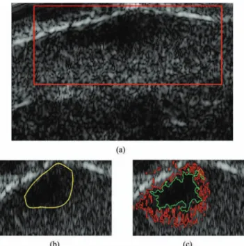
Fig. 8. Log-compressed US images of skin lesion and the corresponding estimated labels (white represents healthy white, red represents lesion) [1]). (a) Dermis view with skin lesion . (b) ROI (slice 2). (c) MRF Labels . (d) Independent Labels .
2) Preliminary 2-D and 3-D Experiments: The two
fol-lowing experiments illustrate the importance of introducing spatial correlation between the mixture components. Fig. 8(a) shows a skin lesion outlined by the red rectangle. This region is displayed with coarse expert annotations (yellow curve) in Fig. 8(b). It should be noted that annotations approximately lo-calize the lesion and do not represent an exact ground truth. The following experiments have been conducted with granularity coefÞcient and the number of classes since there are only two types of tissue (i.e., lesion and healthy reticular dermis) within the region of interest (ROI). The results have been computed from a single Markov chain of 1000 iterations whose Þrst 900 iterations (burn-in period) have been removed.
First, the proposed Bayesian algorithm was used to label each voxel of the ultrasound image as healthy or lesion tissue. The estimated labels obtained using a bidimensional random Þeld are displayed in Fig. 8(c). For comparison purposes, Fig. 8(d) shows the estimation results when labels are considered a priori independent, as in [1]. Due to the proposed MRF prior for the labels, the spatial correlations between image voxels are clearly recovered with the proposed segmentation procedure.
Fig. 9. Log-compressed US images of skin lesion and the corresponding es-timated labels (white represents health, red represents lesion). Images (d)–(f) show the results obtained by considering that voxel labels are independent, as in [1]. Images (g)–(i) show the results obtained with the proposed 3-D Markov random Þeld (MRF) method. (a) ROI (slice 1). (b) ROI (slice 2). (c) ROI (slice 3). (d) Ind. (slice 1). (e) Ind. (slice 2). (f) Ind. (slice 3). (g) MRF (slice 1). (h) MRF (slice 2). (i) MRF (slice 3).
In a second experiment the algorithm was applied in three dimensions using a tridimensional random Þeld. Three slices of the 3-D B-mode image associated with the ROI are shown in Fig. 9(a)–(c). Fig. 9(d)–(f) shows the results obtained when labels are considered a priori independent, as in [1]. The la-bels estimated with the proposed 3-D method are displayed in Fig. 9(g)–(i) where healthy voxels are represented in white and lesion voxels in red. The size of the 3-D images is
voxels. Computing class label estimates using 1000 iterations of the proposed algorithm required 43.5 s (see Section V-C4 for more details about the computational complexity). We observe that most of the MAP labels are in very good agreement with the expert annotations. The improvement obtained when con-sidering correlations in the third dimension can be assessed by comparing Fig. 8(c) and Fig. 9(h), which have been computed from the same data slice. We observe that using a 3-D MRF reduces signiÞcantly the number of misclassiÞcations and im-proves the agreement with the expert annotations.
3) Comparison With a State of the Art Method: The
pro-posed algorithm has been compared with the state of the art method proposed in [25]. This method considers implicitly that the image is a mixture of two Rayleigh components and sep-arates them using an LS algorithm. Comparison has been per-formed with 2-D and 3-D random Þelds. The following experi-ments were conducted with a granularity coefÞcient and a number of classes since there are three types of healthy tissue within the ROI in addition to the lesion. The results have been computed from a single Markov chain of 1000 iterations whose Þrst 900 iterations (burn-in period) have been removed.
Fig. 10(a) shows a skin lesion contained in the ROI outlined by the red rectangle. This region is displayed with coarse ex-pert annotations in Fig. 10(b). The proposed 2-D Bayesian al-gorithm was used to label each voxel of the ROI as healthy or
Fig. 10. Log-compressed US images of skin melanoma tumor and the corre-sponding estimated segmentation contours (green: proposed method, red: [25]).
lesion tissue. Then, from the vector of voxels that were labeled
as lesion we extracted the contour of the largest connected re-gion. The results displayed in Fig. 10(c) show the regular shape of the contour obtained by our method (green curve), whereas the LS method with strong regularization yields a more irreg-ular contour (red curve).
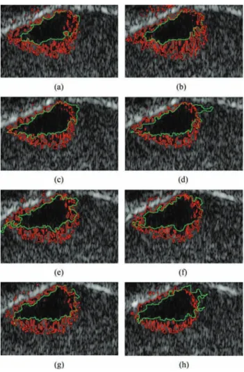
The proposed algorithm was also applied to a 3-D B-mode image using a tridimensional random Þeld. The results for eight slices of the image associated with the ROI depicted in Fig. 10(a) are shown in Fig. 11(a)–(h). The same color code is used for the contours as in the 2-D experiment. The regular shape of the contour obtained by the proposed method is more visible and the recovered lesion Þts better the area depicted by the expert. Finally, Fig. 12 shows a 3-D reconstruction of the lesion’s surface (see [55] for more viewpoints). We observe that the tumor has a semi-ellipsoidal shape which is cut at the upper left by the epidermis–dermis junction. The tumor grows from this junction towards the deeper dermis, which is at the lower right.
Finally, it should be noted that in the in vivo experiments the proposed algorithm has been applied to ROI, as opposed to en-tire 3-D images. This has been motivated by the fact that der-matological ultrasound imaging is used to examine speciÞc re-gions that have been previously identiÞed by the dermatologist. The method presented in this work should be understood in that clinical context and is not intended to be used in unsupervised applications.
4) Computational Complexity: Table II provides averaged
execution times for 500 iterations of the proposed algorithm for several image sizes in 2-D and 3-D and several numbers of classes. The time required to reach convergence can be calcu-lated by multiplying these values by , which corresponds to a burn-in period of 900 iterations. These tests have been computed on a workstation equipped with an Intel Core 2 Duo @2.1 GHz
Fig. 11. 3-D segmentation of an eight-slice image. (a) Slice 1. (b) Slice 3. (c) Slice 5. (d) Slice 7. (e) Slice 9. (f) Slice 11. (g) Slice 13. (h) Slice 15.
Fig. 12. 3-D reconstruction of the melanoma tumor.
processor, 3 MB L2 and 3 GB of RAM memory. The main loop of the Gibbs sampler has been implemented on MATLAB R2010b (The MathWorks Inc., Natick, MA, 2010). However, C-MEX functions have been used to compute the likelihood and to draw samples of from (15). The average execution times of the LS method [25] are provided in [55].
TABLE II
COMPUTINGTIMES(INSECONDS)OF500 ITERATIONS FOR
DIFFERENTIMAGESIZES ANDNUMBER OFCLASSES
VI. CONCLUSION
A spatially coherent Þnite mixture of -Rayleigh distri-butions was proposed to represent the statistics of envelope ultrasound images backscattered from multiple tissues. Spatial correlation was introduced into the model by a Markov random Þeld that promotes dependence between neighbor pixels. Based on the proposed model, a Bayesian segmentation method was derived. Bidimensional and tridimensional implementations of this segmentation method were presented using a Markov chain Monte Carlo algorithm that jointly estimates the un-known parameters of the mixture model and classiÞes voxels into different tissues. The method was successfully applied to several high-frequency 3-D ultrasound images. Experimental results showed that the proposed technique outperforms a state of the art method in the segmentation of in vivo lesions. A tridimensional reconstruction of a melanoma tumor suggested that the resulting segmentations can be used to assess lesion penetration in dermatologic oncology. Future work includes the characterization of the performance of the segmentation algorithm and the study of estimation algorithms for the gran-ularity coefÞcient deÞning the Markov random Þeld prior. A comparison with a maximum likelihood estimator followed by median Þltering is also considered to be an area of interest for potential future work.
ACKNOWLEDGMENT
This work was developed as part of the CAMM4D project, supported by the French FUI and the Midi Pyrenees Regional Council. We would like to acknowledge the support of the Hos-pital of Toulouse, Pierre Fabre Laboratories and Magellium for the ultrasound image acquisition. The authors would particu-larly like to thank Dr. N. Meyer, Dr. S. Lourari, and J. Georges.
REFERENCES
[1] M. A. Pereyra, N. Dobigeon, H. Batatia, and J.-Y. Tourneret, “Labeling skin tissues in ultrasound images using a generalized Rayleigh mix-ture model,” in Proc. IEEE Int. Conf. Acoust., Speech, Signal Proc.
(ICASSP), Prague, Czech Republic, May 2011, pp. 729–732.
[2] M. A. Pereyra, N. Dobigeon, H. Batatia, and J.-Y. Tourneret, “Seg-mentation of ultrasound images using a spatially coherent generalized Rayleigh mixture model,” in Proc. Eur. Signal Process. Conf.
(EU-SIPCO), Barcelona, Spain, Sep. 2011, pp. 664–668.
[3] J. Noble and D. Boukerroui, “Ultrasound image segmentation: A survey,” IEEE Trans. Med. Imag., vol. 25, no. 8, pp. 987–1010, Aug. 2006.
[4] A. Belaid, D. Boukerroui, Y. Maingourd, and J.-F. Lerallut, “Phase-based level set segmentation of ultrasound images,” IEEE Trans. Inf.
Technol. Biomed., vol. 15, no. 1, pp. 138–147, Jan. 2011.
[5] R. Schneider, D. Perrin, N. Vasilyev, G. Marx, P. de Nido, and R. Howe, “Mitral annulus segmentation from 3-D ultrasound using graph cuts,”
IEEE Trans. Med. Imag., vol. 29, no. 9, pp. 1676–1687, Sep. 2010.
[6] K. Somkantha, N. Theera-Umpon, and S. Auephanwiriyakul, “Boundary detection in medical images using edge following algo-rithm based on intensity gradient and texture gradient features,” IEEE
Trans. Biomed. Eng., vol. 58, no. 3, pp. 567–573, Mar. 2011.
[7] P. Yan, S. Xu, B. Turkbey, and J. Kruecker, “Adaptively learning local shape statistics for prostate segmentation in ultrasound,” IEEE Trans.
Biomed. Eng., vol. 58, no. 3, pp. 633–641, Mar. 2011.
[8] G. Unal, S. Bucher, S. Carlier, G. Slabaugh, T. Fang, and K. Tanaka, “Shape-driven segmentation of the arterial wall in intravascular ultra-sound images,” IEEE Trans. Inf. Technol. Biomed., vol. 12, no. 3, pp. 335–347, May 2008.
[9] G. Carneiro, B. Georgescu, S. Good, and D. Comaniciu, “Detection and measurement of fetal anatomies from ultrasound images using a constrained probabilistic boosting tree,” IEEE Trans. Med. Imag., vol. 27, no. 9, pp. 1342–1355, Sep. 2008.
[10] P. Paramanathan and R. Uthayakumar, “Tumor growth in the fractal space-time with temporal density,” in Control, Computation and
Infor-mation Systems, ser. Communications in Computer and InforInfor-mation Science. Berlin, Germany: Springer, 2011, vol. 140, pp. 166–173. [11] K. Horsch, M. L. Giger, L. A. Venta, and C. J. Vyborny, “Automatic
segmentation of breast lesions on ultrasound,” Med. Phys., vol. 28, no. 8, pp. 1652–1659, 2001.
[12] I.-S. Jung, D. Thapa, and G.-N. Wang, “Automatic segmentation and diagnosis of breast lesions using morphology method based on ultra-sound,” in Fuzzy Systems and Knowledge Discovery, L. Wang and Y. Jin, Eds. Berlin, Germany: Springer, 2005, vol. 3614, Lecture Notes in Computer Science, pp. 491–491.
[13] A. Madabhushi and D. Metaxas, “Combining low-, high-level and em-pirical domain knowledge for automated segmentation of ultrasonic breast lesions,” IEEE Trans. Med. Imag., vol. 22, no. 2, pp. 155–169, Feb. 2003.
[14] Y.-L. Huang and D.-R. Chen, “Watershed segmentation for breast tumor in 2-d sonography,” Ultrasound Med. Biol., vol. 30, no. 5, pp. 625–632, 2004.
[15] X. Guofang, M. Brady, J. Noble, and Z. Yongyue, “Segmentation of ultrasound B-mode images with intensity inhomogeneity correction,”
IEEE Trans. Med. Imag., vol. 21, no. 1, pp. 48–57, Jan. 2002.
[16] D. Boukerroui, A. Baskurt, J. Noble, and O. Basset, “Segmentation of ultrasound images-multiresolution 2-D and 3-D algorithm based on global and local statistics,” Pattern Recognit. Lett., vol. 24, no. 4–5, pp. 779–790, 2003.
[17] J. Dias and J. Leitao, “Wall position and thickness estimation from se-quences of echocardiographic images,” IEEE Trans. Med. Imag., vol. 15, no. 1, pp. 25–38, Feb. 1996.
[18] R. Wagner, S. Smith, J. Sandrik, and H. Lopez, “Statistics of speckle in ultrasound B-scans,” IEEE Trans. Sonics Ultrason., vol. 30, no. 3, pp. 156–163, May 1983.
[19] E. Brusseau, C. de Korte, F. Mastik, J. Schaar, and A. van der Steen, “Fully automatic luminal contour segmentation in intracoronary ultra-sound imaging-a statistical approach,” IEEE Trans. Med. Imag., vol. 23, no. 5, pp. 554–566, May 2004.
[20] C. Chesnaud, P. Refregier, and V. Boulet, “Statistical region snake-based segmentation adapted to different physical noise models,” IEEE
Trans. Pattern Anal. Mach. Intell., vol. 21, no. 11, pp. 1145–1157, Nov.
1999.
[21] M. H. R. Cardinal, J. Meunier, G. Soulez, R. L. Maurice, E. Therasse, and G. Cloutier, “Intravascular ultrasound image segmentation: A three-dimensional fast-marching method based on gray level distri-butions,” IEEE Trans. Med. Imag., vol. 25, no. 5, pp. 590–601, May 2006.
[22] S. Osher and J. A. Sethian, “Fronts propagating with curvature-de-pendent speed: Algorithms based on Hamilton-Jacobi formulations,”
J. Comput. Phys., vol. 79, no. 1, pp. 12–49, 1988.
[23] L. Saroul, O. Bernard, D. Vray, and D. Friboulet, “Prostate segmenta-tion in echographic images: A variasegmenta-tional approach using deformable superellipse and Rayleigh distribution,” in Proc. IEEE Int. Symp.
Biomed. Imag. (ISBI), Paris, France, May 2008, pp. 129–132.
[24] F. Destrempes, J. Meunier, M. F. Giroux, G. Soulez, and G. Cloutier, “Segmentation in ultrasonic B-mode images of carotid arteries using mixture of Nakagami distributions and stochastic optimization,” IEEE
Trans. Med. Imag., vol. 28, no. 2, pp. 215–229, Feb. 2009.
[25] A. Sarti, C. Corsi, E. Mazzini, and C. Lamberti, “Maximum likelihood segmentation of ultrasound images with Rayleigh distribution,” IEEE
Trans. Ultrason. Ferroelect. Freq. Contr., vol. 52, no. 6, pp. 947–960,
Jun. 2005.
[26] T. Chan and L. Vese, “Active contours without edges,” IEEE Trans.
Image Process., vol. 10, no. 2, pp. 266–277, Feb. 2001.
[27] F. Lecellier, J. Fadili, S. Jehan-Besson, G. Aubert, M. Revenu, and E. Saloux, “Region-based active contours with exponential family obser-vations,” J. Math. Imag. Vis., vol. 36, pp. 28–45, Jan. 2010. [28] M. A. Pereyra and H. Batatia, “Modeling ultrasound echoes in skin
tissues using symmetric -stable processes,” IEEE Trans. Ultrason.
Ferroelect. Freq. Contr., vol. 59, no. 1, pp. 60–72, Jan. 2012.
[29] F. Y. Wu, “The Potts model,” Rev. Mod. Phys., vol. 54, no. 1, pp. 235–268, Jan. 1982.
[30] O. Eches, N. Dobigeon, and J.-Y. Tourneret, “Enhancing hyperspec-tral image unmixing with spatial correlations,” IEEE Trans. Geosci.
Remote Sens., vol. 49, no. 11, pp. 4239–4247, Nov. 2011.
[31] D. Van de Sompel and M. Brady, “Simultaneous reconstruction and segmentation algorithm for positron emission tomography and trans-mission tomography,” in Proc. 5th IEEE Int. Symp. Biomed. Imag.:
From Nano to Macro, Paris, France, May 2008, pp. 1035–1038.
[32] B. Scherrer, F. Forbes, C. Garbay, and M. Dojat, “Distributed local MRF models for tissue and structure brain segmentation,” IEEE Trans.
Med. Imag., vol. 28, no. 8, pp. 1278–1295, Aug. 2009.
[33] L. Risser, J. Idier, P. Ciuciu, and T. Vincent, “Fast bilinear extrapola-tion of 3-D ising Þeld partiextrapola-tion funcextrapola-tion. Applicaextrapola-tion to fMRI image analysis,” in Proc. ICIP, Cairo, Egypt, 2009, pp. 833–836.
[34] J. Marroquin, E. Santana, and S. Botello, “Hidden Markov measure Þeld models for image segmentation,” IEEE Trans. Patt. Anal. Mach.
Intell., vol. 25, no. 11, pp. 1380–1387, Nov. 2003.
[35] M. Woolrich, T. Behrens, C. Beckmann, and S. Smith, “Mixture models with adaptive spatial regularization for segmentation with an application to fMRI data,” IEEE Trans. Med. Imag., vol. 24, no. 1, pp. 1–11, Jan. 2005.
[36] P. Morse and K. Ingard, Theoretical Acoustics. Princeton, NJ: Princeton Univ. Press, 1987.
[37] D. Salas-Gonzalez, E. E. Kuruoglu, and D. P. Ruiz, “Finite mixture of -stable distributions,” Digit. Signal Process., vol. 19, pp. 250–264, Mar. 2009.
[38] E. E. Kuruoglu and J. Zerubia, “Modeling SAR images with a general-ization of the Rayleigh distribution,” IEEE Trans. Image Process., vol. 13, no. 4, pp. 527–533, Apr. 2004.
[39] A. Achim, E. E. Kuruoglu, and J. Zerubia, “SAR image Þltering based on the heavy-tailed Rayleigh model,” IEEE Trans. Image Process., vol. 15, no. 9, pp. 2686–2693, Sep. 2006.
[40] S. Geman and D. Geman, “Stochastic relaxation, Gibbs distributions, and the Bayesian restoration of images,” IEEE Trans. Patt. Anal. Mach.
Intell., vol. 6, no. 6, pp. 721–741, Nov. 1984.
[41] J. Besag, “Spatial interaction and the statistical analysis of lattice sys-tems,” J. Roy. Stat. Soc., vol. 36, no. 2, pp. 192–236, 1974.
[42] R. Kindermann and J. L. Snell, Markov random Þelds and their
appli-cations. Providence, RI: Amer. Math. Soc, 1980.
[43] Z. Zhou, R. Leahy, and J. Qi, “Approximate maximum likelihood hy-perparameter estimation for Gibbs prior,” IEEE Trans. Image Process., vol. 6, no. 6, pp. 844–861, Jun. 1997.
[44] X. Descombes, R. Morris, J. Zerubia, and M. Berthod, “Estimation of Markov random Þeld prior parameters using Markov chain Monte Carlo maximum likelihood,” IEEE Trans. Image Process., vol. 8, no. 7, pp. 945–963, Jun. 1999.
[45] J. Moller, A. N. Pettitt, R. Reeves, and K. K. Berthelsen, “An efÞcient Markov chain Monte Carlo method for distributions with intractable normalising constants,” Biometrika, vol. 93, no. 2, pp. 451–458, Jun. 2006.
[46] C. McGrory, D. Titterington, R. Reeves, and A. Pettitt, “Variational Bayes for estimating the parameters of a hidden Potts model,” Stat.
Comput., vol. 19, pp. 329–340, 2009.
[47] C. P. Robert and G. Casella, Monte Carlo Statistical Methods. New York: Springer-Verlag, 1999.
[48] A. P. Dempster, N. M. Laird, and D. B. Rubin, “Maximum likelihood from incomplete data via the EM algorithm,” J. R. Stat. Soc., vol. 39, no. 1, pp. 1–38, 1977.
[49] J. Diebolt and E. H. S. Ip, “Stochastic EM: Method and application,” in Markov Chain Monte Carlo in Practice, W. R. Gilks, S. Richardson, and D. J. Spiegelhalter, Eds. London, U.K.: Chapman & Hall, 1996. [50] N. Dobigeon and J.-Y. Tourneret, “Bayesian orthogonal component analysis for sparse representation,” IEEE Trans. Signal Process., vol. 58, no. 5, pp. 2675–2685, May 2010.
[51] N. Dobigeon, A. Hero, and J.-Y. Tourneret, “Hierarchical Bayesian sparse image reconstruction with application to MRFM,” IEEE Trans.
Image Process., vol. 18, no. 9, pp. 2059–2070, Sep. 2009.
[52] T. Vincent, L. Risser, and P. Ciuciu, “Spatially adaptive mixture mod-eling for analysis of fMRI time series,” IEEE Trans. Med. Imag., vol. 29, no. 4, pp. 1059–1074, Apr. 2010.
[53] K. Kayabol, E. Kuruoglu, and B. Sankur, “Bayesian separation of im-ages modeled with MRFs using MCMC,” IEEE Trans. Image Process., vol. 18, no. 5, pp. 982–994, May 2009.
[54] M. Mignotte, “Image denoising by averaging of piecewise constant simulations of image partitions,” IEEE Trans. Image Process., vol. 16, no. 2, pp. 523–533, Feb. 2007.
[55] M. Pereyra, N. Dobigeon, H. Batatia, and J.-Y. Tourneret, Segmenta-tion of skin lesions in 2-D and 3-D ultrasound images using a spatially coherent generalized Rayleigh mixture model Univ. Toulouse, France, IRIT/INP-ENSEEIHT, 2011 [Online]. Available: http://pereyra.perso. enseeiht.fr/pdf/Pereyra_TMI_TR_2011.pdf
[56] J. Gonzalez, Y. Low, A. Gretton, and C. Guestrin, “Parallel Gibbs sam-pling: From colored Þelds to thin junction trees,” in Proc. Artif. Intell.
Stat. (AISTATS), Ft. Lauderdale, FL, May 2011.
[57] G. O. Roberts, “Markov chain concepts related to sampling algo-rithms,” in Markov Chain Monte Carlo in Practice, W. R. Gilks, S. Richardson, and D. J. Spiegelhalter, Eds. London, U.K.: Chapman Hall, 1996, pp. 259–273.
[58] Z. Sun and C. Han, “Heavy-tailed Rayleigh distribution: A new tool for the modeling of SAR amplitude images,” in Proc. IEEE Int. Geosci.
Remote Sens. Symp., Boston, MA, Jul. 2008, vol. 4, pp. 1253–1256.
[59] C. L. Nikias and M. Shao, Signal Processing with Alpha-Stable
Distri-bution and Applications. New York: Wiley, 1995.
[60] A. Gelman and D. Rubin, “Inference from iterative simulation using multiple sequences,” Stat. Sci., vol. 7, no. 4, pp. 457–511, 1992. [61] C. P. Robert and S. Richardson, “Markov chain Monte Carlo methods,”
in Discretization and MCMC Convergence Assessment, C. P. Robert, Ed. New York: Springer Verlag, 1998, pp. 1–25.
[62] A. Gelman, J. B. Carlin, H. P. Robert, and D. B. Rubin, Bayesian Data
Analysis. London, U.K.: Chapman Hall, 1995.
[63] T. Hergum, S. Langeland, E. Remme, and H. Torp, “Fast ultrasound imaging simulation in k-space,” IEEE Trans. Ultrason. Ferroelect.
Freq. Contr., vol. 56, no. 6, pp. 1159–1167, Jun. 2009.
[64] T. Szabo, Diagnostic Ultrasound Imaging. Boston, MA: Academic, 2004.

![Fig. 8. Log-compressed US images of skin lesion and the corresponding estimated labels (white represents healthy white, red represents lesion) [1]).](https://thumb-eu.123doks.com/thumbv2/123doknet/3633806.106946/9.892.465.828.385.698/compressed-images-corresponding-estimated-labels-represents-healthy-represents.webp)