Identification et optimisation des propriétés dynamiques des matériaux viscoélastiques

(1)

m WlVBRStrfijM

1 3 SHERBROOKE

Faculte de genie

Departement de genie mecanique

IDENTIFICATION ET OPTIMISATION DES PROPRIETES DYNAMIQUES DES MATERIAUX VISCOELASTIQUES

These de doctorat Specialite: genie mecanique

Zhiyong REN

Jury : Francois CHARRON (rapporteur) Noureddine ATALLA (directeur) Raymond Panneton

Franck SGARD Sebastian GHINET

(2)

**1*1**

Library and Archives Canada Published Heritage Branch Bibliothgque et Archives Canada Direction du Patrimoine de l'6dition 395 Wellington Street Ottawa ON K1A 0N4 Canada 395, rue Wellington Ottawa ON K1A 0N4 Canada

Your file Votre reference ISBN: 978-0-494-62821-8 Our file Notre reference ISBN: 978-0-494-62821-8

NOTICE: AVIS:

The author has granted a

non-exclusive license allowing Library and Archives Canada to reproduce, publish, archive, preserve, conserve, communicate to the public by

telecommunication or on the Internet, loan, distribute and sell theses

worldwide, for commercial or non-commercial purposes, in microform, paper, electronic and/or any other formats.

L'auteur a accorde une licence non exclusive permettant a la Bibliotheque et Archives Canada de reproduce, publier, archiver, sauvegarder, conserver, transmettre au public par telecommunication ou par I'lnternet, preter, distribuer et vendre des theses partout dans le monde, a des fins commerciales ou autres, sur support microforme, papier, electronique et/ou autres formats.

The author retains copyright ownership and moral rights in this thesis. Neither the thesis nor substantial extracts from it may be printed or otherwise reproduced without the author's permission.

L'auteur conserve la propriete du droit d'auteur et des droits moraux qui protege cette these. Ni la these ni des extraits substantiels de celle-ci ne doivent etre imprimis ou autrement

reproduits sans son autorisation.

In compliance with the Canadian Privacy Act some supporting forms may have been removed from this thesis.

While these forms may be included in the document page count, their removal does not represent any loss of content from the thesis.

Conformement a la loi canadienne sur la protection de la vie privee, quelques formulaires secondares ont ete enleves de cette these.

Bien que ces formulaires aient inclus dans la pagination, il n'y aura aucun contenu

manquant.

(3)

IDENTIFICATION AND OPTIMIZATION OF THE DYNAMIC

PROPERTIES OF VISCOELASTIC MATERIALS

ABSTRACT

In the automotive, railway and aerospace industries, interior noise is an important consideration in design and operation. Among the available technologies to reduce the structure-borne vibration and noise, the use of Metal-Polymer Sandwich (MPS) panels is attracting more interest from Original Equipment Manufacturers (OEMs). As for constrained-layer damping (CLD) treatments, besides developing more accurate models (theoretical and finite element) to simulate the vibroacoustic performance, it is very important to accurately identify the properties of the constituent materials of an MPS. Since the core materials in MPS exhibit viscoelastic properties which vary significantly with temperature and frequency, it is necessary to develop experimental and/or optimization methods to characterize the dynamic properties so that they may be well matched to specific noise and vibration control applications. This is the objective of this thesis. In this thesis, a simple free-free beam based setup, together with an identification algorithm has been developed to identify the dynamic properties of core materials from the measured frequency response functions. The setup involved circumventing some drawbacks of the traditional clamped-free setup. In particular, a new optimization method is brought forward wherein a four-parameter fractional derivative model plus a three-parameter Williams-Landel-Ferry (WLF) equation are used to describe the temperature and frequency dependent behaviour of core materials. Therefore, few parameters are optimized for the temperature and frequency dependent properties. The objective function in the optimization is based on the so-called amplitude correlation coefficient which can be calculated directly by the frequency response functions. The normal mode superposition method taking the added mass into account, as well as Ross-Kerwin-Ungar (RKU) equations, as a solver, is used to calculate the predicted frequency response functions. The Pattern Search algorithm is used to find the best values of design parameters. This algorithm is a global optimization algorithm and is less sensitive to the initial values of design parameters.

Numerical examples and tests on several MPS panels were used to validate the free-free setup and optimization method by systematic comparison with the ASTM E756-04 Standard and with DMA when the latter is possible. However, with some MPS panels, the proposed method failed to provide satisfactory results. It was further postulated that the manufacturing process of these MPS panels may somehow have modified the properties or the constitutive law of the polymer itself.

Keywords: viscoelastic materials, constrained-layer damping treatments, optimization, dynamic properties

(4)

IDENTIFICATION ET OPTIMISATION DES PROPRIETES

DYNAMIQUES DES MATERIAUX VISCOELASTIQUES

RESUME

Dans les industries automobiles, ferroviaires et aerospatiales, le bruit interieur est une consideration importante dans la conception et le fonctionnement. Parmi les technologies permettant de reduire les vibrations et les bruits d'origine solidien, les panneaux sandwich metal-polymere -metal (MPS) ont de plus en plus d'applications. Pour les traitements

amortissant contraints, en plus de developper des modeles plus precis (theorique et

elements finis) pour simuler les performances vibroacoustiques, il est tres important d'identifler les proprietes du polymere constituant le coeur du MPS. Etant donne que ce coeur presente des proprietes viscoelastiques qui varient de fa?on significative avec la temperature et la frequence, il est necessaire de mettre au point des methodes experimentale et/ou d'optimisation pour caracteriser precisement les proprietes dynamiques de sorte qu'ils puissent etre bien adapte au controle du bruit et des vibrations. C'est l'objectif de cette these. Elle a permis de developper une methode d'identification basee sur un montage du poutre de libre libre et une methode d'optimisation operant directement sur directement les fonctions de reponse en frequence mesurees a differentes temperatures. En particulier, la methode d'optimisation utilise le modele de derivee fractionnaire a quatre parametres ainsi que 1'equation Williams-Landel-Ferry (WLF') de trois parametres pour decrire la loi de comportement du polymere en fonction de la temperature et de la frequence permettant ainsi de limiter 1'optimisation a peu de parametres.

Des exemples numeriques et plusieurs mesures sur des MPS sont presentes pour illustrer la validite de la methode d'identification proposee. En particulier, lorsque possible, une comparaison systematiquement avec la norme en vigueur (ASTM E756-04) et la methode

DMA est presentee. Toutefois, pour certains MPS, la methode proposee ne donne pas de

resultats satisfaisants. II est alors possible d'imaginer que le processus de fabrication du MPS ait pu modifier les proprietes ou la relation contrainte-deformation du polymere.

Mots Cles: materiaux viscoelastiques, traitements amortissant contraints, optimisation, proprietes dynamiques

(5)

ACKNOWLEDGEMENTS

I would like to express my gratitude to my supervisor, Professor Noureddine Atalla, for his valuable advice, interest, encouragement and guidance throughout the duration of this project.

I would like to thank my past and present colleagues of GAUS, especially Dr. Sebastian Ghinet, who by their enthusiasm and their fruitful discussions provided insight into related fields of interest and an enjoyable working environment.

I also highly appreciate the members of the jury, Professors Francois Charron, Noureddine Atalla, and Raymond Panneton, and Drs. Franck Sgard and Sebastian Ghinet, for evaluating my research and providing valuable comments and advice.

Special thanks are due to my family for their love and support. Without them this thesis would not have been brought to completion.

(6)

LIST OF FIGURES

Figure 1.1 Damping applications in the automotive body structure 2 Figure 1.2 Classical models of viscoelastic behaviour: (a) Maxwell (b) Voigt (c)

standard 6 Figure 1.3 Variation of storage modulus and loss factor of a viscoelastic material

with temperature 10 Figure 1.4 Free layer damping 13

Figure 1.5 Constrained layer damping 14 Figure 1.6 Free layer treatment (non-deformed and deformed) 15

Figure 1.7 Constrained layer treatment (non-deformed and deformed) 16

Figure 1.8 Iterative modal strain energy algorithm 21

Figure 2.1 How a DMA works 33 Figure 2.2 DMA data and master curves (a) modulus versus frequency (b) master

curves 36 Figure 2.3 Test specimens (1) bare beam specimen (2) Oberst beam specimen (3)

modified Oberst beam specimen (4) sandwich beam specimen 37 Figure 2.4 Experimental setup with clamped-free configuration 38

Figure 2.5 Cantilever beam used in the Standard 41 Figure 2.6 Similarity between a free-free beam excited in its center and a

cantilever beam excited by its base 42

Figure 2.7 WJP setup 43 Figure 2.8 VBT with free-free configuration for mobility measurement 44

Figure 2.9 Experimental setup: (a) added mass (b) input mobility (c) Data

acquisition system 45 Figure 2.10 Frequency-dependent complex added mass: (a) amplitude (b) phase 46

Figure 2.11 Experimental and corrected input mobilities: (a) 10°C (b) 30°C (for

each subfigure, the top is for bare beam and the bottom for sandwich beam) 47

Figure 2.12 Added mass: (a) amplitude (b) phase 48 Figure 2.13 Experimental and corrected data for aluminum beams: (a) Aluminum

1 (b) Aluminum 2 (c) Aluminum 3 (d) Aluminum 4 49 Figure 2.14 Young's modulus and loss factors for four aluminum beams: (a)

modulus versus frequency (b) loss factor versus frequency 49 Figure 2.15 Added mass, experimental and corrected input mobilities for skin and

sandwich beams: (a) mass (amplitude) (b) mass (phase) (c) input mobilities of

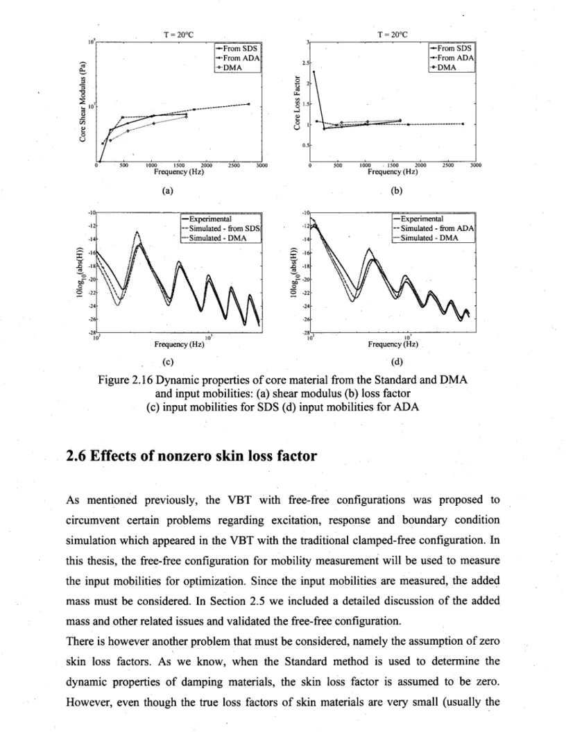
steel and SDS (d) input mobilities of aluminum and ADA 52 Figure 2.16 Dynamic properties of core material from the Standard and DMA and

(10)

Figure 2.17 Reference dynamic mechanical properties of the core material 55

Figure 2.18 Clamped-free configuration 55 Figure 2.19 Comparison of the reference and Standard results for zero skin loss

factor: (a) 7,= - 1 0oC ( b ) r = 1 0 ° C ( c ) 7,= 30°C(d) master curves 58

Figure 2.20 Comparison of the reference and Standard results for the 0.007 skin

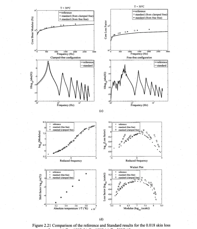
loss factor: (a) T= -10°C (b) T= 10°C (c) T = 30°C (d) master curves 60 Figure 2.21 Comparison of the reference and Standard results for the 0.018 skin

loss factor: (a) T= -10°C (b) T= 10°C (c) T= 30°C (d) master curves 62

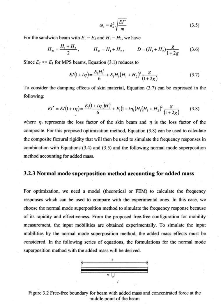
Figure 3.1 Comparison of the Standard and proposed methods 66 Figure 3.2 Free-free boundary for beam with added mass and concentrated force

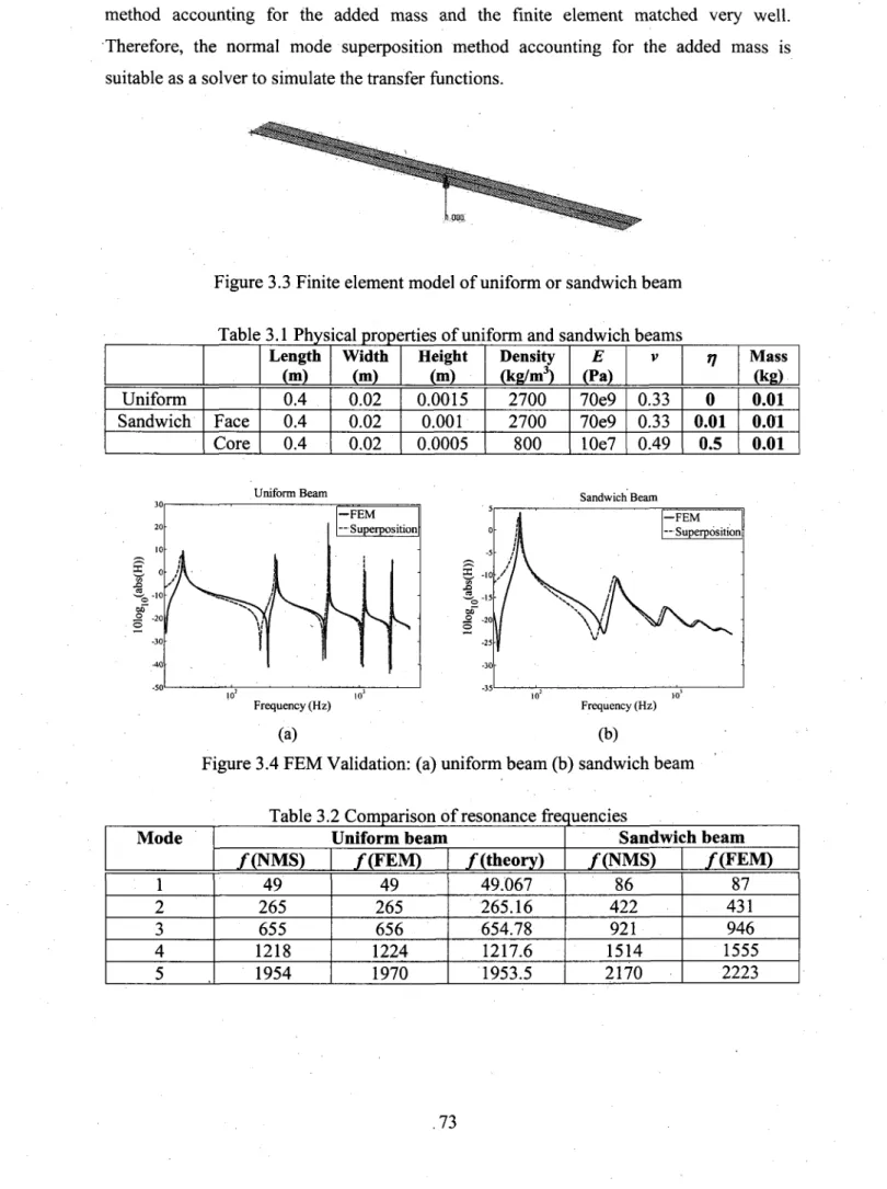
at the middle point of the beam 69 Figure 3.3 Finite element model of uniform or sandwich beams 73

Figure 3.4 FEM Validation: (a) uniform beam (b) sandwich beam 73

Figure 3.5 Proposed method 79 Figure 3.6 Shear modulus and loss factors of PIB: (a) shear modulus (b) loss

factors 85 Figure 3.7 Comparison of the reference, optimization and Standard results for

PIB: (a) 0°C (b) 20°C (c) 30°C (d) master curves using optimized WLF (e) master

curves using reference WLF 87 Figure 3.8 Comparison of the reference, optimization and Standard results for the

material for zero skin loss factor: (a) -10°C (b) 10°C (c) 30°C (d) master curves 92 Figure 3.9 Comparison of the reference, optimization and Standard results for the

material for the 0.007 skin loss factor: (a) -10°C (b) 10°C (c) 30°C (d) master

curves 94 Figure 3.10 Comparison of the reference, optimization and Standard results for

the material for the 0.018 skin loss factor: (a) -10°C (b) 10°C (c) 30°C (d) master

curves 96 Figure 3.11 Master curves using the reference ('*'), optimized ( ' • ' ) and Standard

('o') data for various skin loss factors: (a) zero skin loss factor (b) 0.007 skin loss

factor (c) 0.018 skin loss factor 97 Figure A.l Dynamic properties of core material (at glassy region): (a) shear

modulus (b) loss factor 101 Figure A.2 Input mobilities of 50 samples at -10°C: (a) 10% (b) 25% 101

Figure A.3 Dynamic properties of core material (at transition region): (a) shear

Figure A.5 Dynamic properties of core material (at rubbery region): (a) shear

(11)

Figure 4.1 Optimized Young's modulus and loss factors and comparison of bare

beam input mobilities: (a) 8°C (b) 32°C 106 Figure 4.2 Comparison of dynamic properties of core material and sandwich input

mobilies: (a) 8°C (b) 16°C (c) 24°C (d) 32°C 110 Figure 4.3 Master curves of core material: (a) core shear modulus (b) core loss

factors ('o' and ' • ' represent the core properties from the optimization and

Standard, respectively) 111 Figure 4.4 Optimized Young's modulus and loss factors and comparison of bare

beam input mobilities: (a) 0°C (b) 30°C 112 Figure 4.5 Comparison of dynamic properties of core material and sandwich input

mobilities: (a) 0°C (b) 10°C (c) 20°C (d) 40°C 115 Figure 4.6 Master curves of Deltane 350: (a) core shear modulus (b) core loss

factors ('*', 'o' and ' • ' represent the optimization, Standard and DMA data,

respectively) 116 Figure 4.7 Comparison of dynamic properties and sandwich input mobilities: (a)

core Young's modulus (b) core loss factors (c) input mobilities (solid line,' ', ' ' and • - ' represent the input mobilities obtained from the experiment,

optimization, Standard and DMA data, respectively) 117 Figure 4.8 Optimized Young's modulus and loss factors and comparison of bare

beam input mobilities: (a) 16°C; (b) 32°C 119 Figure 4.9 Comparison of dynamic properties of core material and experimental

and simulated input mobilities at typical temperatures (a) 16°C; (b) 32°C 121 Figure 4.10 Master curves of material T: (a) core shear modulus; (b) core loss

factors ('o' and '*' represent the data from optimization and Standard,

respectively) 122 Figure 4.11 Dynamic properties of core material and experimental and simulated

input mobilies: (a) 0°C; (b) 40°C (for input mobilities, solid line, ' . . . ' and ' — ' represent the input mobilities obtained from the experiment, optimization and

Standard data, respectively) 123 Figure 4.12 Master curves of A l l : (a) core shear modulus (b) core loss factors

('o' and '*' represent the optimization and Standard data, respectively) 124

Figure 4.13 Master curves for the Standard results 125 Figure 4.14 Dynamic properties of core material and experimental and simulated

input mobilies: (a) 0°C; (b) 40°C (for input mobilities, solid line, ' .', ' - - ' and ' - • - ' represent the input mobilities obtained from the experiment, optimization,

Standard and DMA data, respectively) 126 Figure 4.15 Master curves of A l l : (a) core shear modulus; (b) core loss factor

('o', '*' and ' • ' represent the optimization, Standard and DMA data, respectively) 127 Figure 4.16 Dynamic properties of core material and experimental and simulated input mobilities: (a) 0°C (b) 40°C (solid line, ' ', and ' - represent the input mobilities obtained from the experiment, optimization, and Standard data,

(12)

Figure 4.17 Master curves of M i l : (a) core shear modulus (b) core loss factors

('o' and '*' represent the optimization and Standard data, respectively) 130

Figure 4.18 Master curves for standard results 130 Figure 4.19 Dynamic properties of core material and experimental and simulated

input mobilies: (a) 0°C; (b) 40°C (solid line, ' ' and ' — ' represent the input mobilities obtained using the experiment, optimization and Standard data,

respectively) 131 Figure 4.20 Master curves of M i l : (a) core shear modulus; (b) core loss factors

(13)

LIST OF TABLES

Table 1.1 Automotive applications 2 Table 2.1 Summary of techniques and calculations used to determine dynamic

mechanical properties 34 Table 2.2 Comparison of DMA and VBT 40

Table 2.3 Geometrical and physical properties of aluminum beams 48 Table 2.4 Geometrical and physical properties of the steel/Deltane 350/steel beam 50

Table 2.5 Geometrical and physical properties of the aluminum/Deltane

350/aluminum beam 50 Table 2.6 Geometrical and physical properties of the MPS beam (clamped-free

configuration) 54 Table 2.7 Geometrical and physical properties of the MPS beam (free-free

configuration) 54 Table 3.1 Physical properties of uniform and sandwich beams 73

Table 3.2 Comparison of resonance frequencies 73

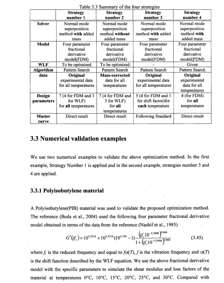
Table 3.3 Summary of the four strategies 84 Table 3.4 Geometrical and physical properties of skin and sandwich beams and

core material 85 Table 3.5 Initial, identified and reference parameters for the material 88

Table 3.6 Comparison of some parameters for reference and optimization 89 Table 3.7 Geometricaland physical properties of the sandwich beam 89 Table A. 1 Geometrical and physical properties of the structure 100 Table 4.1 Geometrical and physical properties of beams A and C and core

material 105 Table 4.2 Geometrical and physical properties of base, sandwich beams and core

material 111 Table 4.3 Geometrical and physical properties of bare, sandwich beams and T 118

Table 4.4 Geometrical and physical properties of material A l l 122 Table 4.5 Geometrical and physical properties of material Ml 1 128

(14)

CHAPTER 1 INTRODUCTION

1.1 Backgrounds

Interior noise is an important consideration in the design and operation of automotive, railway and aerospace vehicles. Interior noise in automobiles is mainly due to the vibration of different systems such as floor panels, body panels* engine mounts and suspensions, under various excitations (engine, power train, road inputs, wind, etc.). The vibration of these components is responsible for about 90% of the harshness-related acoustical energy in the vehicle interior. The interior noise is primarily controlled by the properties and complexity of the panels responsible for the acoustic radiation and the effectiveness of the attached soundproofing and damping materials. However, modern weight and space constraints require the optimal use of these materials and thus the development of new noise and vibration control strategies (Atalla, 2005). Vibration and noise in a dynamic system can be reduced by a number of means. These can be broadly classified into active, passive, and semi-active methods. Active control involves the use of certain active elements such as speakers, actuators, and microprocessors to produce an "out-of-phase" signal to electronically cancel the disturbance. The traditional passive control methods for airborne noise include the use of absorbers, barriers, mufflers, silencers, etc. For reducing structure-borne vibration and noise, several methods are available. Sometimes just changing the system's stiffness or mass to alter the resonance frequencies can reduce the unwanted vibration as long as the excitation frequencies do not change. But in most cases, the vibrations need to be isolated or dissipated by using isolator or damping materials. In semi-active methods, active control is used to enhance the damping properties of passive elements. Examples include electro-rheological (ER) and magneto-rheological (MR) fluids, and active constrained layer damping (ACLD) in which the traditional constraining layer is replaced by a smart material. The full-scale implementation of active and semi-active control technology in vehicles and commercial airplanes has been slowed down because of the high costs and the complexity of the sound field in the cabin interior.

Passive damping is, in general, simpler to implement and more cost-effective than semi-active and semi-active techniques which require on-line control. Damping can be added to a system by using special viscoelastic materials in a number of ways (Rao, 2002). Passive damping as a technology has been dominant in the non-commercial aerospace industry

(15)

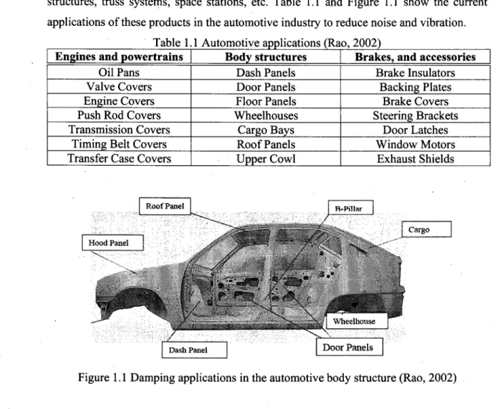
since the early 1960s. Advances in materials technology, along with newer and more efficient analytical and experimental tools for modeling the dynamic behaviour of materials and structures have led to many applications such as inlet guide vanes of jet engines, helicopter cabins, exhaust stacks, satellite structures, equipment panels, antenna structures, truss systems, space stations, etc. Table 1.1 and Figure 1.1 show the current applications of these products in the automotive industry to reduce noise and vibration.

Engines and powertrains Body structures Brakes, and accessories

Oil Pans Dash Panels Brake Insulators

Valve Covers Door Panels Backing Plates

Engine Covers Floor Panels Brake Covers

Push Rod Covers Wheelhouses Steering Brackets

Transmission Covers Cargo Bays Door Latches

Timing Belt Covers Roof Panels Window Motors Transfer Case Covers Upper Cowl Exhaust Shields

Figure 1.1 Damping applications in the automotive body structure (Rao, 2002)

For optimal passive damping treatments, damping can be added explicitly in the form of added treatments (spray, baked-on mastics, asphalt sheets, viscoelastic constrained layer patches, tuned viscoelastic dampers, etc.), embedded in the design of the structure (laminated steel), or indirectly added through the use of sound packages (damping added by foams, fibres, etc.). Damping treatments are believed to be most effective in reducing structure-borne noise at low frequencies. At high frequencies, they work in conjunction with the sound package to reduce air-borne transmission paths. Currently, the actual damping treatment and its nature vary with vehicle platforms and overall Original

(16)

There is a need to develop a robust strategy to select, locate and optimize the damping treatment over broader frequencies and temperatures. The first step into this direction concentrates on constrained and free layer treatments with an emphasis on Metal-Polymer Sandwich (MPS) panels. Indeed, the recent scale availability and use of steel/polymer/steel sandwich panels has motivated the need for the development of accurate prediction methods for vibration and acoustic performance. Optimizing and designing such materials requires a detailed and fundamental investigation of the mechanisms of damping materials and their interaction with the underlying vibration structures.

1.2 Objectives of the thesis

This thesis is part of a larger effort by the Groupe d'Acoustique et de Vibrations de 1'Universite de Sherbrooke (GAUS) to develop in-depth knowledge of MPS panels and optimize their structural characteristics and vibroacoustic performance. The main objective is to develop, implement and validate a simple hybrid experimental-numerical method to identify the dynamic properties of polymer cores used in MPS panels. The specific tasks are:

(1) Use of an experimental setup with free-free configuration for mobility measurement to obtain the accurate experimental input mobilities of MPS panels. In particular, the setup circumvents the drawbacks of the current ASTM E756-04 standard;

(2) Development of an optimization method to accurately identify the dynamic mechanical properties of viscoleastic materials sandwiched between two metal beams, by directly using the measured frequency response functions at various temperatures. Applying the temperature-frequency superposition principle, this optimization method should provide the temperature and frequency dependent properties of viscoelastic materials in the form of a nomogram (master curves); (3) Validate and discuss the advantages and limitations of the proposed method using

various MPS and viscoleastic materials. A systematic comparison with the ASTM E756-04 Standard method and DMA when available should be used to make the comparison.

(17)

1.3 Literature review

1.3.1 Damping mechanism

Damping refers to the extraction of mechanical energy from a vibrating system, usually by conversion of this energy into heat. Damping serves to control the steady-state resonant response and to attenuate traveling waves in the structures. There are two types of damping: material damping and system damping. Material damping is the damping inherent in the material, while system or structural damping includes the damping at the supports, boundaries, joints, interfaces, etc., in addition to material damping. Various terms such as viscous damping, hysteretic damping, Coulomb damping, linear and proportional damping, etc. are used in the literature to represent vibration damping. There are various damping mechanisms available. One is the linear viscous damping mechanism, in which the viscous damping is linear so that the observed response does not change qualitatively as the amplitude of excitation increases, but only changes amplitude by the same ratio as the excitation changes. Another is the internal material damping mechanism which comes into play when metals, alloys and many other structural materials are deformed during vibration. This mechanism of damping is often very complex, and depends upon the metallurgical processing of the alloy as well as the exact composition (Zener, 1937, 1948, Nowick, 1953, Kimball et al., 1927, Lazan 1968). There is another damping mechanism, known as nonlinear friction damping which is very different from both viscous and internal material damping. When two rigid plane surfaces are in contact and slide along one another, the forces of interaction are generally very complex, arising from an extremely large number of interactions between microscopic 'hills' and 'valleys' during the sliding motion. It is generally neither feasible nor profitable to analyse such interactions in great detail, because this would require knowledge of the microscopic surface features, which is generally unavailable. Sliding friction can be used as a damping mechanism in vibrating systems, and can sometimes be very effective, particularly at high temperatures where other mechanisms may not be effective or desirable. However, the nonlinear nature of the equations of motion does lead to greater mathematical complications than are generally encountered. For details, see the references (Barron et al.,

(18)

Viscoelastic damping is a property exhibited by a wide variety of polymeric materials, ranging from natural or synthetic rubbers, through various adhesives to industrial plastics. Due to the long-range molecular order associated with their giant molecules, polymers and elastomers exhibit rheological behaviour intermediate between a crystalline solid and a simple liquid. Of particular importance is the marked dependence of both stiffness and damping on frequency and temperature. These polymeric materials offer a wide range of possibilities for producing the desired levels of damping in structures and machines, provided that the designers have sufficient understanding of the mechanical behaviour features which must be exploited efficiently in any damping design process.

1.3.2 Modeling the dynamic mechanical behaviour of viscoelastic

materials

There are many models to describe the mechanical behaviours of viscoelastic materials, such as the complex modulus model, Maxwell model, Kelvin-Voigt model, the standard model which combines the Maxwell and Kelvin-Voigt model, fractional derivative model (Nashif et al., 1985, Jones, 2005, Ferry, 1970, Williams, 1964, Bagley et al„ 1979, 1983, Rouse, 1953, Ferry et al. 1955, Caputo, 1971, Bagley et al., 1979, 1983, 1986, Rogers, 1983, Torvik et al., 1984, 1987, Pritz, 1996, 2003) and the Havriliak-Negami (HN) model (Havriliak et al., 1966), etc.

When the strain-time history and the stress-time history are both harmonic, there exists a time or phase lag between the strain and the corresponding stress. For a viscoelastic solid, the phase lag implies that a velocity dependent term exists in the stress-strain relationship. The complex modulus model is motivated by observing the relationship between sinusoidal stress and sinusoidal strain in viscoelastic materials. The strain lags the stress and the imaginary part of the complex constant adequately describes this phenomenon. The limitation of the complex modulus model is that it is restricted to sinusoidal motion of the material. Crandall has shown that application of this method to the general motion of the material leads to serious mathematical problems (Jones, 2005, Bagley et al., 1983 Crandall, 1963)

There are some mathematical models to describe the behaviours of rheological systems. The simplest ones are single-parameter models: (i) an idealized spring which exhibits a restoring force linearly proportional to displacement and thus displays no damping

(19)

whatsoever, and (ii) an idealized dashpot, which produces a force linearly proportional to velocity. Obviously, neither of these models is adequate in representing the behaviour of most real materials.

k ki

c k2 c2

(a) Maxwell model (b) Voigt model (c) Standard model

Figure 1.2 Classical models of viscoelastic behaviour: (a) Maxwell (b) Voigt (c) standard

The next most complicated models of rheological systems are the two-parameter models: (i) the Maxwell model, which consists of a spring and dashpot mechanical series and (ii) the Kelvin-Voigt model, which is comprised of a spring in parallel with a dashpot, as shown in Figure 1.2. The Maxwell model is a fair approximation to the behaviour of a viscoelastic liquid. However, as a model for a viscoelastic solid, it has several very serious drawbacks (Lazan, 1968): there are no means to provide for internal stress and for afterworking. The Kelvin-Voigt model overcomes these deficiencies and is a first approximation to the behaviour of a viscoelastic solid. However, it has the following disadvantage (Lazan, 1968): there is no elastic response during application or release of loading; the creep rate approaches zero for long durations of loading; and there is no permanent set irrespective of the loading history. It should be mentioned that the Kelvin-Voigt model is the simplest one which permits representation as a complex quantity when subjected to sinusoidal motion.

The standard 'classical' element, a combination of both Maxwell and Voigt elements, is a three-parameter model and models with many parameters and different combinations of both Maxwell and Voigt elements also appear. When only a very few elements are involved in the models, calculations are relatively simple, but the agreement with observed behaviour is usually poor, since the constant dashpot coefficient used implies a far too rapid variation of complex modulus properties with frequency. When distributions representing an infinite number of infinitesimal elements are used, the agreement with

(20)

a finite but substantial number of elements, typically from four to ten, does allow for modeling real complex modulus behaviour quite well, but a large number of parameters must be identified, and this can be quite tedious, though by no means impossible. An excellent account of the development of the classical models, based on spring-dashpot elements, for describing viscoelastic material behaviour has been provided by Williams (Williams, 1964).

The classical models are still of valuable theoretical interest. However, modeling viscoelastic material behaviour has been greatly simplified in recent years, particularly with respect to the frequency domain, using the fractional derivative model instead of the classical approach. The fractional derivative model is based on the observed mechanical behaviour of many materials (Bagley et al. 1983). It is important to note that there is a link between molecular theories that predict the macroscopic behaviour of certain viscoelastic media and the fractional calculus approach to viscoelasticity. These molecular theories include the molecular theory for a dilute polymer solution developed by Rouse (Rouse, 1953), and modified by Ferry, Landed and Williams (Ferry et al., 1955) for concentrated polymer solution and for polymer solids. The existence of a theoretical basis would be of substantial significance to the engineering application of these models, for it would enhance the degree of confidence with which one could extend their application to other materials and to other loading conditions (Bagley 1983).

The general form of the fractional derivative viscoelastic model is:

where D" <•> represents the a-order time derivative of the quantity; a„, and are fractional numbers; Eq and Et are material parameters. In Equation (1.1), the

time-dependent stress fields are related to time-time-dependent strain fields through series of derivatives of fractional order. Experimental observations indicated that many viscoelastic materials could be modeled by retaining only the first fractional derivative term in each series in Equation (1.1). The result is a viscoelastic model with five parameters: b, Eo, E\,

a and /?. After transforming the equation from time domain to frequency domain, the

fractional derivative constitutive equation can be expressed as

M N

(J{t) + < <7(0 >= E0s(t) +^EnDa" < £{t) > (1.1)

m=1

(21)

where a and s are the stress and strain in frequency domain, to is angular frequency, and

i is the square root of -1. This model suggests that the frequency dependent modulus is a

function of fractional powers of frequency. The five parameters are determined by a least squares fit of this model to the frequency-dependent mechanical properties of the material. In many cases, taking a = (5produced a very satisfactory fit (Bagley et al., 1983).

The fractional derivative models have proven to be a powerful tool in describing the dynamic behaviour of various materials, namely metals, geological strata and glass (Caputo et al., 1971), especially polymers for vibration control (Bagley, 1979, 1983, Rogers, 1983, Bagley et al., 1979, 1984, Torvik et al., 1987). The advantage of the fractional derivative models is not only their capability for describing real dynamic behaviour, but that they are causal and simple enough for engineering calculations. Moreover, it has been established that the fractional derivative model with only four parameters can be used for describing the variation of dynamic elastic and damping properties in a wide frequency range, provided that there is only one loss peak (Pritz, 1996); and the fractional derivative model with five parameters can be used to describe asymmetrical loss factor peak and the high-frequency behaviour of polymeric damping materials (Pritz, 2003).

Another five parameter model was developed by Havriliak and Negami (HNM) (Havriliak et al., 1966). It is also the most widely used equation to describe the viscoelastic behaviour of materials. The complex shear modulus G* in HNM can be expressed in the following

where Go and Gx are the lower and upper limits of dynamic shear modulus; / a n d fo are the

analysis and reference frequencies and 0 < a and /? < 1. When a = p, it is equivalent to the four parameter fractional derivative model.

1.3.3 Behaviours and typical properties of polymeric materials

Unlike many other damping mechanisms, such as those discussed in the previous section, most homogeneous isotropic polymeric materials exhibit damping behaviour which depends strongly upon temperature and frequency, but is linear with respect to vibration equation:

(22)

and cross-linked molecular chains, each containing thousands or even millions of atoms. The internal molecular interactions which occur during deformation in general, and vibration in particular, give rise to macroscopic properties such as stiffness and energy dissipation during cyclic deformation, which is the damping mechanism for polymers. The specific mechanical behaviour of each polymeric compound is intimately related to the structure of the molecular chains and the links between adjacent chains. When a polymer specimen is subjected to a load, such as a step load, the molecules are disturbed from their initial equilibrium positions and, over time, they rearrange until a new equilibrium state is reached which creates the internal forces needed to balance the applied load. The time required to approach a specified close approximation to this state, for example 99%, is finite and depends on temperature as well as composition. Similarly, if the specimen is subjected to harmonically varying (sinusoidal) loads, the molecules will after some time reach a state of 'dynamic equilibrium' and respond 'in sympathy' with the exciting load. Again, the time to reach this state depends upon temperature and composition, but in this case it will also depend upon the frequency.

Effects of temperature

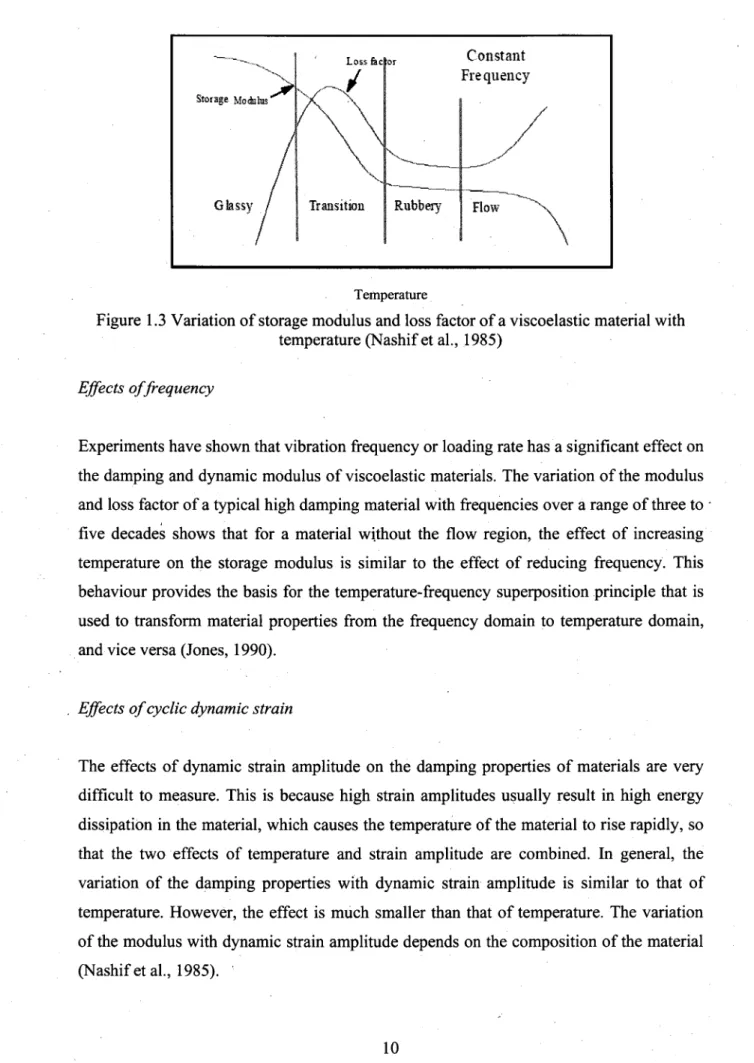
The temperature is perhaps the most important environmental factor affecting the dynamic properties of damping materials. This effect is shown in Figure 1.3 for a typical polymeric material with four distinct regions. The first region is the glassy state where the material has a very large storage modulus (dynamic stiffness) but very low damping. The storage modulus in this region changes slowly with temperature, while the loss.factor changes significantly with increasing temperature. In the transition region where the material changes from a glassy state to a rubbery state, the material modulus decreases rapidly with increasing temperature because the material softens and this increases the loss factor. Damping usually peaks at or around the glass transition temperature of the material. Some polymers can be made to have more than one transition region by changing the polymeric structure and composition to take advantage of the peak damping capacity in this region. In the rubbery state both the modulus and loss factor take somewhat low values and vary rather slowly with temperature. The flow region is typical for a few damping materials such as vitreous enamels and thermoplastics, where the material continues to soften as the temperature increases while the loss factor reaches very high values.

(23)

Constant Frequency

Rubbery Flow

\

Temperature

Figure 1.3 Variation of storage modulus and loss factor of a viscoelastic material with temperature (Nashif et al., 1985)

Effects of frequency

Experiments have shown that vibration frequency or loading rate has a significant effect on the damping and dynamic modulus of viscoelastic materials. The variation of the modulus and loss factor of a typical high damping material with frequencies over a range of three to five decades shows that for a material without the flow region, the effect of increasing temperature on the storage modulus is similar to the effect of reducing frequency. This behaviour provides the basis for the temperature-frequency superposition principle that is used to transform material properties from the frequency domain to temperature domain, and vice versa (Jones, 1990).

. Effects of cyclic dynamic strain

The effects of dynamic strain amplitude on the damping properties of materials are very difficult to measure. This is because high strain amplitudes usually result in high energy dissipation in the material, which causes the temperature of the material to rise rapidly, so that the two effects of temperature and strain amplitude are combined. In general, the variation of the damping properties with dynamic strain amplitude is similar to that of temperature. However, the effect is much smaller than that of temperature. The variation of the modulus with dynamic strain amplitude depends on the composition of the material (Nashif et al., 1985).

(24)

Effects of static preload

The effects of static preload on the dynamic properties of materials are usually most important in the rubbery region. In general, the modulus increases with increasing preload, whereas the loss factor decreases (Nashif et al., 1985).

Other environmental effects

Not only do the complex modulus properties of polymers vary with frequency, temperature and strain amplitude, usually in a reversible manner, but various factors in the operational environment can lead to irreversible changes in the complex modulus. For example, exposure to hydrocarbon fluids, such as fuels and lubricants, may progressively and irreversibly damage the molecular structure over time, and this will be reflected as changing complex modulus behaviour with respect to temperature, frequency and strain, as well as deteriorating tensile, shear and tear strengths.

Other environmental factors of concern include radiation (ultraviolet or nuclear, for example) and humidity in the atmosphere surrounding the application. If radiation is present, the damage may be progressive. If it is a case of humidity, the process may in some cases be reversible. In all cases, realistic simulations of expected operating conditions can establish whether particular damped products or systems will behave adequately.

The Combined effects of temperature and frequency (Nashif et al., 1985, Jones, 2001)

Using classical characterization methods for viscoelastic materials, the number and range of frequency and temperature data points are limited. It is therefore clear that the process of interpolation to intermediate temperatures, or extrapolation to frequencies outside the measured range could not readily be performed in a direct manner with any degree of accuracy. However, it is often more appropriate to apply the concept of temperature-frequency equivalence (also known as the temperature-temperature-frequency superposition principle). The major hypothesis on which the principle of temperature-frequency equivalence is based is the assumption that complex modulus values at any chosen frequency f and any

(25)

chosen (reference) temperature T\ are identical to those at any other frequency^ at some different temperature T2 which must be selected, so that:

G* ( / , , T]) = G* {f2a(T2)) (1.4)

where ciTi) is to be determined. The factor fa(T) describes a simple operation combining the effect of both frequency and temperature into a single variable, which is referred to as the reduced frequency.

The two most popular shift factors «(7) are used to describe the temperature-frequency superposition principle: WLF (Williams-Landel-Ferry) and Arrhenius Equations. The WLF equation can be expressed (ASTM E756-04, 2005):

iog1 0[«(r)] = c , J (1.5)

C2+T-T0

where Ci and C2 are constants, and To is the reference temperature, all to be determined for the specific material. The reference temperature To can be chosen arbitrarily, but note that the values of the other parameters which best fit the test data will vary with the value chosen for Tq.

The Arrhenius shift factor relationship is written as (ASTM E756-04, 2005): log w[a(T)] = TA

vT tqJ

(1.6) where T is the current temperature and T0 is any arbitrarily selected reference temperature

(both in absolute degrees). TA is the activation temperature and it is related to the activation

energy. In most practical cases, the difference between the 'best-fit' WLF equation and the 'best-fit' Arrhenius equation is not very great (Jones, 2001 and ASTM E756-04, 2005). Once the parameters of the WLF or Arrhenius equations are obtained, the master curves (also known as the nomogram) which can display the modulus and loss factors in one diagram and make the data easy to be read will be created (ASTM E756-04, 2005).

1.3.4 Damping treatment design

Generally, viscoelastic materials are used to enhance the damping of a structure in two different ways: free-layer damping treatment and constrained-layer or sandwich-layer damping treatment. Although these designs have been used for over forty years, recent improvements in the understanding and application of the damping principles, together

(26)

successful applications. The key point in any design is to recognize that the damping material must be applied in such a way that it is significantly strained whenever the structure is deformed in the vibration mode under investigation.

Free-Layer Damping (FLD)

Figure 1.4 illustrates a portion of a structure with a free-layer, which is sometimes called extensional type damping treatment. The damping material is either sprayed on the structure or bonded using a pressure-sensitive adhesive. Examples include undercoating of automobiles and application of "mastics" to body and floor panels to provide damping. When the base structure is deflected in bending, the viscoelastic material deforms primarily in extension and compression in planes parallel to the base structure. The hysteresis loop of the cyclic stress and strain dissipates the energy. The degree of damping is limited by thickness and weight restrictions.

Dam ping Material

Base Structure /

Figure 1.4 Free layer damping (Jones, 1996)

The vibration analysis of a beam with a viscoelastic layer was first conducted by Kerwin and his colleagues (Kerwin, 1959, Ross et al., 1959). The viscoelastic characteristic of the material was modeled using the complex modulus approach. The system loss factor in a free-layer system increases with the thickness, storage modulus, and loss factor of the viscoelastic layer. Another interesting feature of the free-layer treatment is that the damping performance is independent of the mode shape of vibration for full coverage by the viscoelastic layer. It is however possible to optimize partial coverage for a particular mode or a limited number of modes (Lall et al., 1988, Kung et al., 1999).

Constrained-Layer Damping (CLD)

Figure 1.5 shows an arrangement of a constrained-layer damping treatment. This consists of a sandwich composed of two outer elastic layers with a viscoelastic material as the core.

(27)

When the base structure undergoes bending vibration, the viscoelastic material is forced to deform in shear because of the upper stiff layer. The constrained-layer damping is more effective than the free-layer design since more strain energy is consumed and dissipated into heat in the work done by the shearing mode within the viscoelastic layer. The symmetric configuration in which the base and the constraining layers have the same thickness and stiffness is by far the most effective design as it maximizes the shear deformation in the core layer. The constrained-layer design can simply be extended to include a) a stand-off damper in which a spacer is used in between the viscoelastic material and the base layer, and b) multiple damping layers, which are very effective for obtaining damping over wider temperature and frequency ranges.

Constraining layer ~ Damping Material

Base Structure

Figure 1.5 Constrained layer damping (Jones, 1996)

1.3.5 Theoretical and numerical models for sandwich and laminated

structures

There are many theoretical and numerical models to represent the mechanical behaviours of sandwich and laminated structures. The best known theoretical models have been put forward by Oberst (Oberst et al., 1952), Ross, Kerwin and Ungar (RKU) (Kerwin, 1959, Ross et al., 1959), DiTaranto (DiTaranto,1965), Mead and Markus (Mead et al., 1969), Yan and Dowell (Yan et al., 1972), Yu (Yu, 1962) and Ghinet and Atalla (Ghinet 2005). Mead (Mead 1983) provided a good review of the previous theories (DiTaranto, 1965, Mead et al., 1969, Yan et al., 1972). Among the best known numerical models are: the Golla-Hughes-McTavish (GHM) model; the Augmenting Thermodynamic Fields (ATF) model; the Anelastic Displacement Fields (ADF) model; the Augmented Hooke's Law (AHL) model; the Iterative Modal Strain Energy model, the Amichi and Atalla model (Amichi et al. 2009) and the Shorter's Spectral Finite Element Model (Shorter, 2004), among others.

(28)

The Oberst Equations

Oberst appears to have been the first to investigate and apply free layer damping treatments (Oberst et al., 1952). He published a set of equations describing the damping contribution of a free layer damping treatment applied to a beam or plate, the 'Oberst equations', and used them to predict the performance of such damping treatments, and in reverse, to predict the damping properties of polymers from measurements of vibrating beams coated with the treatment.

i A i B ^ Polymer y

Metal 'A' 'B'

Undeformed Deformed

Figure 1.6 Free layer treatment (non-deformed and deformed) (Jones, 1996)

Figure 1.6 shows the configuration of a free layer treatment in the deformed and non-deformed states. The Oberst equations are based on the assumption that plane sections remain plane and the amplitudes of vibration are small, as illustrated. The Oberst equation in complex format is then usually written as:

EI (1 + iJj) = 1 + e2h2 (1 + irj2) + 3(1 + h2)' e 2h2 (1 + it]2) 1 + e2h2 (l + irj2) (1.7) V i

where Hi, E\, p\ and H2, £2, pi are the thicknesses, Young modulus and densities of base beam and polymer material, respectively; h2 = H2 / H\, and e2 = E2 / E\. It is clear that, for

free layer treatments, both e2 and h2 should be as large as possible, at least up to a certain

point. The Oberst equations, while strictly applicable only to complete coverage of non-stiffened beams or plates, are very useful even today for making rapid estimates of the effect of free layer treatments on modal damping, even for complex structures.

The RKU Equations (Jones, 1996, Ross etal., 1959, Kerwin, 1959)

Ross, Kerwin and Ungar appear to be the first to have published an analysis of a constrained layer treatment on a beam or plate (Ross et al., 1959). Mead (Richards et al.,

(29)

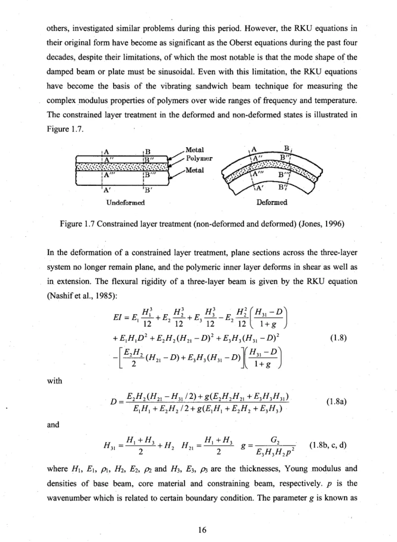
others, investigated similar problems during this period. However, the RKU equations in their original form have become as significant as the Oberst equations during the past four decades, despite their limitations, of which the most notable is that the mode shape of the damped beam or plate must be sinusoidal. Even with this limitation, the RKU equations have become the basis of the vibrating sandwich beam technique for measuring the complex modulus properties of polymers over wide ranges of frequency and temperature. The constrained layer treatment in the deformed and non-deformed states is illustrated in Figure 1.7. >A <B j A " }R" 1 A'f j zv 1 1 jB'" 'A' Undeformed 'B' Metal Polymer Metal

Figure 1.7 Constrained layer treatment (non-deformed and deformed) (Jones, 1996)

In the deformation of a constrained layer treatment, plane sections across the three-layer system no longer remain plane, and the polymeric inner layer deforms in shear as well as in extension. The flexural rigidity of a three-layer beam is given by the RKU equation (Nashif etal., 1985): „ , _ M? _ H\ _ H EI = E, + E2 -2- + — 1 12 2 12 3 12 3 -H. 12 1 + g + EXHXD2 + E2H2(H2X -D)2 + E3H3{H3X -D)2 E-.H {H2X-D) + E3H3{H3X-D) with and D E2H2(H2l -H3X /2) + g(E2H2H2l +E3H3H31) ElHl+E2H2/2 + g(ElHl +E2H2 +E3H3) Hn=——l + H2 H2l HX+H3 g = -(1.8) (1.8a) (1.8b, c, d) 2 . 2 E3H3H2p

where H\, E\, p\, H2, E2, pi and Hj, E-}, pi are the thicknesses, Young modulus and densities of base beam, core material and constraining beam, respectively, p is the

(30)

the shear parameter. Due to the deformation mechanisms, the constrained layer damping treatment is more effective than the free layer damping treatment.

Other Theoretical Models

To establish the complex stiffness Equation (1.8) of a composite beam, Kerwin (Kerwin, 1959) put forward to the following assumptions: (1) for the beam cross section, there was a neutral axis, whose location varies with frequency; (2) there was no slipping between the elastic and viscoelastic layers at their interfaces; (3) the major part of the damping was due to the shearing of the viscoelastic material, whose shear modulus was represented as

G* = Gc(l + it]); (4) the elastic layers displaced laterally by the same amount; (5) the beam

was simply supported and vibrated at a natural frequency, or the beam was infinitely long so that the end effects (beam fixation) could be neglected. Using the first four of the abovementioned considerations, DiTaranto (DiTaranto, 1965) proposed a sixth-order, complex, homogeneous differential equation in terms of the longitudinal displacement at the constrained elastic layer for the free vibrations of a three-layer beam. Damping of the beam is due to the complex shear modulus of the viscoelastic material. The solution of this sixth-ordef, complex, homogeneous differential equation subject to satisfying boundary conditions, yields the desired natural frequencies and associated composite loss factors. Based on the assumptions that shear strains in the face-plates are negligible, that longitudinal direct stresses in the core are negligible, and that transverse direct strains in both core and face-plates are also neglected, Mead and Markus (Mead et al., 1969) derived a sixth-order differential equation of motion in terms of the transverse displacement (other than the longitudinal displacement in DiTaranto's paper) for a three-layer sandwich beam with a viscoelastic core. They also found the mathematical expressions in terms of the transverse displacement for a variety of beam boundary conditions.

Yan and Dowell (Yan et al., 1972) developed a fourth-order equation of motion for beams and plates. The face-plates' shear deformation effects, and longitudinal and rotary inertia were included to obtain sixth-order equations and then neglected so as to obtain a simplified four-order equation of motion.

Mead (Mead, 1983) reviewed the previous theories of Yan and Dowell, DiTaranto, and Mead and Markus and stated that most authors have made the same basic assumptions: (i) the core which carried shear, but no direct stress, was linearly viscoelastic and had the

(31)

complex shear modulus Gc{\+irj)\ (ii) the face-plates were elastic and isotropic and

suffered no shear deformation normal to the plate surfaces; (iii) the inertia forces of transverse flexural motion were dominant, with negligible longitudinal and rotary inertia of the face-plates and core; (iv) all points On a normal to the plate moved with the same transverse displacement; (v) no slip occurred at the interfaces of the core and face-plates. This set of assumptions is termed in the literature as the Mead and Markus (MM) model. In the reference (Mead 1983), special attention is devoted to the simplified Yan and Dowell model as well as the DiTaranto and the Mead and Markus models to be validated and compared with a more accurate differential equation that account for shearing and rotational inertia in the face-plates as well as a discrete displacement field of the layers. Mead also discussed the conditions and the ranges of validity for these models in comparison with the new accurate theory. He pointed out that the DiTaranto and the Mead and Markus equations yield reliable values provided the flexural wavelength is greater than about four face-plate thicknesses. The Yan and Dowell equations yield reliable values only at much greater wavelengths or when the central layer in the sandwich is very thick (Mead 1983).

An analytical method considering flexural, longitudinal, rotational and shear deformations ' in all layers of sandwich beams with multiple constrained layer damping patches was

proposed by Kung and Singh (Kung et al., 1999). The method was verified by comparing results for a single patch with those reported in the literature by Lall (Lall et al., 1988) and Rao (Rao, 1978). Examples of experimental validation were also presented.

Recently, two wave-based approaches have been proposed by Ghinet and Atalla (Ghinet 2005). The first concerned the modeling of a thick flat sandwich composite; it used a discrete displacement field for each layer and allowed for out-of-plane displacements and shearing rotations. Good results were obtained compared to experimental data. The second concerned the modeling of thick laminate structures. Each layer was described by a Reissner-Mindlin displacement field, and equilibrium relations accounted for membrane, transversal shearing, bending, and the full inertial terms. The discrete displacement of each layer led to accuracy over a wide frequency range. The model was successfully validated with numerical classical spectral finite elements and experimental results.

The analysis procedures discussed above are useful for examining the basic mechanisms of surface damping treatments and are applicable to problems involving specialized geometry, loadings, and boundary conditions. Even for simple geometries, algebraic or

(32)

numerical solution of the problem tends to be complicated and lengthy. In any case, these methods are not usable when the base beam or plate is a generally laminated composite (except Ghinet and Atalla (Ghinet 2005)). Practical problems usually involve complicated structural geometries and boundary conditions, and only a portion of the structure has damping treatment applied to it. Since much of the difficulty of analyzing a constrained layer damping treatment is due to complicated geometries, it is normal, as in the case of undamped structures, to look at finite element techniques for solutions to the problems. Using the finite element method, arbitrary boundary conditions and loadings can be modeled quite easily.

To apply finite element analysis to the sandwich or laminated structures with viscoelastic cores, the key problems are the description of constitutive relationships of viscoelastic cores and the selection of elements of face and core structures. Another consideration is the computational cost. It is also an important issue.

Among the finite element analysis of sandwich and/or laminated structures, Golla-Hughes-McTavish (GHM) model (Golla et al., 1985, Golla-Hughes-McTavish et al., 1992, 1993) is the most famous one to model the viscoelastic structures. The GHM model represented sandwich and laminate structures with a viscoelastic core by introducing internal variables to account for viscoelastic relaxation and, thus, damping behaviour. The material shear modulus function in the model can be represented as a series of mini-oscillatory terms, in the Laplace domain, as follows (McTav-ish et al., 1993)

sG(s) = G( l + Z ai (1-9)

^ V s2+2^o)iS + cof J

where Gx represents the relaxed modulus, or static modulus. It should be noted that, from

(1.9), the unrelaxed modulus may be written as G0 = Gx( 1 + ^ . a , ) . Each mini-oscillatory

term in the series is dependent on three material constants, namely a, , col and C,t,

evaluated from curve-fitting of the viscoelastic material master curves. This method allows for both a good representation of the frequency-dependence of viscoelastic materials and time-domain analyses of the augmented systems, since all of its matrices are constants. The Augmenting Thermodynamic Fields (ATF) modeling method (Lesieutre, 1989, 1992, Lesieutre et al., 1989, 1991) was a time-domain continuum model of material damping that preserved the characteristic frequency-dependent damping and modulus of real materials. Motivated by results from materials science, the augmenting thermodynamic fields were introduced to interact with the usual mechanical displacement field. The methods of

(33)

irreversible thermodynamics were used to develop coupled material constitutive relations and partial differential equations of evolution. These equations were implemented for numerical solution within the computational framework of the finite element method. Like GHM, ATF employed additional coordinates to more accurately model damping. The primary difference between the ATF method and the GHM method is that ATM is a direct time-domain formulation, not transform-based, and yields finite elements using conventional methods. In addition, the 'dissipation coordinates' of GHM are internal to individual elements, while the augmenting fields of ATF are continuous from element to element, reflecting its basis as a field theory. Finally, because it was intentionally developed with second-order dynamics, the GHM method was quite compatible with current analysis methods, and has proven to be useful in practice. However, because of its second-order form, GHM is perhaps less efficient as a general model of material behaviour.

The Anelastic Displacement Fields (ADF) model, proposed in these references (Lesieutre et al., 1995, 1996a, 1996b, Bianchini et al., 1995), was a time domain model for linear viscoelasticity. It was based on a decomposition of the total displacement field into two parts: elastic and anelastic. The anelastic displacement field was used to describe that part of the strain that was not instantaneously proportional to stress. The coupled material constitutive equations described the relationships between the total and anelastic stresses and the corresponding strains. The differential equations governing the behaviour of anelastic displacement field (relaxation equations) were developed in a form similar to those that governed the behaviour of a total displacement field (equations of motion), both involving the divergence of appropriate stress tensor. The boundary conditions for the total displacement field are the familiar ones of elastodynamics. The anelastic displacement field is effectively an internal field, as it is driven exclusively through coupling to the total displacement field, and could not be directly affected by applied loads. Because the total displacement field and the anelastic displacement fields can be treated similarly, the ADF model has led to more direct finite element development.

Dovstam (Dovstam, 1995) proposed an isothermal, fully three-dimensional material damping modelling technique, to some extent an alternative to classic viscoelasticity. The method is formulated in the frequency domain as an augmented Hooke's law (AHL) with a constitutive matrix in which material damping was introduced by adding frequency dependent, complex valued terms to the classical material modulus matrix of Hooke's

(34)

directly implemented, as a complex valued constitutive matrix, in any finite element code incorporating complex node variables, complex element (material) properties and a complex equation solver. Spatial (i.e. element) and frequency dependent damping could be introduced in finite element models in a natural way without need for extra degrees of causality freedom. Problems in the damping description were avoided completely because the basic assumptions were formulated in the time domain, even though the resulting AHL formulation was a frequency domain method. Numerical tests and comparisons to one-dimensional analytical solutions have been done with quite satisfactory results. For a more detailed review of the above models, see reference (Trindade et al., 2000).

Bagley and Torvik (Bagley et al., 1983) introduced the fractional derivative model to the viscoelastical materials and applied this model to the analysis of viscoelastically damped structures combined with the finite element method. Galucio, Deu and Ohayon (Galucio et al., 2004) proposed a finite element formulation of viscoelastic sandwich beams using fractional derivative operators. In their model, the sandwich configuration was composed of a viscoelastic core (based on Timoshenko theory) sandwiched between elastic faces (based on Euler-Bernoulli assumptions). The viscoelastic model used to describe the behaviour of the core was a four-parameter fractional derivative model. To solve the equation of motion, a direct time integration method based on the implicit Newmark scheme was used. Numerical applications showed its effectiveness.

Figure 1.8 Iterative modal strain energy algorithm (Trindade et al., 2000)

Another method, known as the iterative modal strain energy model (Trindade et al., 2000) has also been proposed. In this model, the modal loss factor is approximated as the product of the viscoelastic material loss factor by the fraction of the dissipative energy, present in

(35)

the viscoelastic material, to the total strain energy. Following this definition, the iterative algorithm is proposed in Figure 1.8. Using this algorithm, undamped eigenfrequencies and eigenvectors can be correctly evaluated and a good approximation for modal low damping is obtained. In this method, the convergence was very fast, however, evaluation must be repeated for each frequency of interest.

The above discussed the finite element method of sandwich structures with viscoelastic core. Several constitutive relations about the viscoelastic core materials have been brought forward to apply the finite element methods to the sandwich structures. Another important issue is the selection of the finite elements for sandwich structures. The classical modeling strategy uses solid elements for both the core and the skins. To save the cost of computation, the combination of beam (or plate, shell) elements and solid elements is used to discretize the sandwich structures. The beam (or plate, shell) elements are used for elastic face structures and the solid elements for viscoelastic core materials. In these cases, the beam (or plate, shell) element must be offset to account for coupling between stretching and bending deformation. Reference (Sun et al., 1995) by Sun and Lu has provided a detailed discussion on this issue. Further discussion can be found in references (Plouin et al., 2000, Balmes et al., 2002a, 2002b, 2004).

Some authors have used the existing general purpose finite element analysis codes (such as MSC/NASTRAN) to study the sandwich structures with viscoelastic cores. Johnson and Kienholz (Johnson et al., 1982) used solid elements (Hexa8) for the viscoelastic core and quadrilateral thick shell element (Quad4) with offsets for the face sheets. Soni (Soni, 1981) used isoparametric thin shell elements (8-20 nodes) for the face sheets and solid elements (Hexa8) for the viscoelastic core that were fully compatible. Experimental data demonstrated these two methods on simple problems with good results. However, Mace (Mace, 1994) criticized these approaches as being too complex and costly to use. He developed a model based on the sandwich beam theory. His finite element analysis focused on a sandwich beam with only a very thin viscoelastic layer. He used five degrees of freedom per node. Good results were obtained compared to numerical methods. However, it was found to be less accurate compared to Johnson et al.'s method (Johnson et al., 1982). Moreover, Baber et al (Baber et al., 1998) presented a finite element model derived in much the same manner as the Mace model. It allowed for both thin and moderately thick viscoelastic cores and was accurate over a wide range of frequencies. However, this model contains 12 degrees of freedom per element so it is costly to use.