Any correspondence concerning this service should be sent to the repository administrator:
[email protected]
Identification number: DOI: 10.1016/j.ymssp.2014.01.006
Official URL:
http://dx.doi.org/10.1016/j.ymssp.2014.01.006
This is an author-deposited version published in:
http://oatao.univ-toulouse.fr/
Eprints ID: 11047
To cite this version:
Picot, Antoine and Obeid, Ziad and Régnier, Jérémi and Poignant, Sylvain and
Darnis, Olivier and Maussion, Pascal Statistic-based Spectral Indicator for
Bearing Fault Detection in Permanent-Magnet Synchronous Machines using the
Stator Current. (2014) Mechanical systems and signal processing, vol. 46 (n°
2-3). pp. 424-441. ISSN 0888-3270
O
pen
A
rchive
T
oulouse
A
rchive
O
uverte (
OATAO
)
OATAO is an open access repository that collects the work of Toulouse researchers and
makes it freely available over the web where possible.
Statistic-based spectral indicator for bearing fault detection
in permanent-magnet synchronous machines using
the stator current
A. Picot
a,n, Z. Obeid
a, J. Régnier
a, S. Poignant
b, O. Darnis
b, P. Maussion
aa
Université de Toulouse, CNRS, INPT, UPS, LAPLACE (Laboratoire Plasma et Conversion d'Energie), ENSEEIHT, 2 rue Charles Camichel, BP 7122, F-31071 Toulouse cedex 7, France
bSAFRAN-Technofan, 10, place Marcel Dassault, BP 30053, ZAC du Grand Noble 31702 Blagnac cedex, France
Keywords:
Current-based diagnostic Bearing fault detection Synchronous machine Current spectral analysis Student's t test Welch's periodogram
a b s t r a c t
In this paper, an original method for bearing fault detection in high speed synchronous machines is presented. This method is based on the statistical process of Welch's periodogram of the stator currents in order to obtain stable and normalized fault indicators. The principle of the method is to statistically compare the current spectrum to a healthy reference so as to quantify the changes over the time. A statistic-based indicator is then constructed by monitoring specific harmonic family. The proposed method was tested on two experimental test campaigns for four different speeds and compared to a vibration indicator. The method was evaluated using a rigorous perfor-mance evaluation metric. A threshold evaluation was performed and shows that the proposed method is very tolerant to the machine speed. Thus, the use of a unique fault threshold whatever the speed can be considered. Results showed excellent agreement as compared with the vibration indicator, with an overall correlation of r ¼0.74 and only 4% of false alarms. Performance demonstrated by this novel method was superior to those of a classical energy-based indicator in terms of correlation with the vibration indicator and detection stability. Moreover, results also showed a better robustness of the proposed method since good performance can be obtained with the same detection threshold whatever the speed or the measure campaign whereas it needs to be redefined for each case with the classical indicator. This work shows the advantages of a statistic-based approach in order to increase the robustness of bearing fault detection in permanent-magnet synchronous machines.
1. Introduction
Over the past few years, electrical machines are more and more used in many industrial applications. So, monitoring has become an important industrial research area in order to assess their safety and reliability. There are a lot of different causes for failures in electrical machines such as eccentricity, load torque oscillations, and stator turn short circuit. A review of these different causes can be found in[1]. Among them, it has been shown in[2]that ball bearing defects are responsible for 40% of machine failures. Bearing faults can lead to critical events such as abnormal temperature or vibration level, rotor
http://dx.doi.org/10.1016/j.ymssp.2014.01.006
nCorresponding author.
locking, or stator friction. Therefore, manufacturers show more and more interests in monitoring their health state in order to guarantee the availability and the predictive maintenance in actuator elements like machine for example.
Bearing faults are part of mechanical defaults. So, the first approach used to monitor bearing faults has been to analyze the vibrations of electrical machines. The traditional technique is to monitor characteristic frequencies of specific bearing damages in the vibration spectrum as presented in [3–5]. The spectrum is generally computed using the Fast Fourier Transform (FFT). These techniques imply however to know precisely the resonance frequencies for bearing faults and a mathematical of model of the machine is often needed to identify them. This point can be partly solved using the Spectral Kurtosis in order to detect the frequency bands with the maximum impulsivity[6]. Other representation modes have been proposed such as wavelet [7]or Empirical Mode Decomposition [8] in order to detect changes in the vibration spectral content. The statistical analysis of the spectral content has also been proven to be very efficient with tools such as Spectral Kurtosis evaluating the distribution of different frequency components[9]or more recently extreme value theory evaluating the distribution of spectrum excesses[10].
Nevertheless, the expensive cost of vibration sensors (such as piezoelectric accelerometers) makes these solutions often difficult to implement. Consequently, several studies [11–13] have successfully suggested to process the stator current signals. One of the advantages is that stator current measurements are often available in electrical machines for control purposes. In the same way as vibration signals, specific signatures linked to bearing faults appear on the stator current spectrum. A general review of the different techniques based on the stator current spectrum analysis is presented in[14]. These techniques are mainly based on the analysis of the stator current spectral content assessed by time–frequency[13,15] or time-scale techniques[16]. Recent works have shown that statistical approaches such as Spectral Kurtosis[6,17]were very efficient to monitor machine faults. These detection techniques mainly concern the induction machine. However, a few work deals with bearing fault detection in permanent magnet machines[16,17].
Energy-based methods have been proved to be efficient in order to dissociate healthy and faulty cases afterwards but they are often very weak when it comes to predict which threshold value to use. Statistical approaches have proven to be efficient to overcome this issue as statistic-based indicators can be normalized[10,18,19]. More details on the computation details of the main bearing diagnostic approaches are given in[20]. Moreover, most of these works only deal with one type of machine at a certain speed and the question of reproducibility (for different speeds, for different machine of a same type) is very rarely addressed. From this point of view, the statistical approach presented in[18]shows encouraging results using center-reduced variables.
This paper focuses on bearing fault detection for a high speed permanent magnet synchronous machine PMSM belonging to an air conditioning fan used in aeronautic. Classical stator current signatures related to the vibration bearing frequencies are not suitable for such applications due to their low level. However, some frequencies multiple of the rotation frequency in the stator current spectrum have been proved to be sensitive to the considered faults [17]. Here, an indicator based on center-reduced spectral components is proposed. The interest of such a methodology is to normalize the different frequency components in order to detect and evaluate significant modifications of the spectrum without any a priori knowledge on healthy and faulty levels for the different spectral components. This technique is tested on 2 different experimental campaigns, for 4 different speeds.
The outline of the paper is the following.Section 2starts with a description of the experimental test bench and protocol, followed by a description of theoretical signatures of bearing defects on the current spectrum. The traditional energetic indicator as well as the proposed statistic-based indicator are then detailed. The evaluation protocol is presented at the beginning ofSection 3. The optimization of the proposed method as well as the results obtained with energy-based and statistic-based indicators are presented in this section. These results are then compared and discussed inSection 4.
2. Materials and methods
2.1. System description and experimental protocol
The studied system is an air conditioning fan (Technofan LP2). It is used in most of the commercial aircrafts to provide air conditioning and renewing. The whole fan is showed in Fig. 1a. Its power is 5 kVA and its maximum speed Vmax is
14,100 rpm (rotations per minute).
This machine consists of a high-speed permanent magnet synchronous machine with sinusoidal back electromotive forces and fed by a pulse width modulation (PWM) current source inverter operating sequentially to provide 1201 square wave currents in the three phases. The block diagram of the whole system is depicted inFig. 2where Ibus, Iinv, and I1;2;3are
respectively the DC bus current, the inverter current, and the stator current for the 3 phases, Icis the capacitor current and Ve
is the inverter speed used for the system regulation. This kind of control avoids using an accurate position sensor such as a resolver. The PWM is synchronized thanks to three Hall effect sensors. Cris the resistant torque of the machine.
The experimental protocol is separated into two measurement parts. The first part is performed with a healthy bearing, and the second one with a faulty bearing. The faulty bearing is artificially aged by a burning grease process at 200 1C during 60 h and a broken cage. This protocol of degradation has been designed by machine industrial specialists from the fan manufacturer SAFRAN-Technofan in order to be representative of real bearing degradations. This protocol was designed as part of the PREMEP project[21]. Moreover, it guarantees a vibrational level very close to the healthy level for several hours
of operation before the first signs of failure. Two test campaigns have been conducted with bearings having followed the same degradation protocol. The experimental bench is presented inFig. 1b and c.
Current signals are measured by a PowerDNA Ethernet acquisition system PPC8, with 3 ! 4 18-bit analog inputs DNA-AI-205 with a sampling frequency of 200 kHz. Data are recorded every hour for 5 s. The measurements have been performed for 4 different mechanical rotation speeds: 8000, 10,000, 12,000 and 14,100 rpm. Data are stored in the text format using LABVIEW, and then converted into the MATLAB format for usage.
For the first campaign, the whole dataset consists of 200 recordings in the healthy case and 487 recordings in the faulty case. For the second campaign on the same machine but with different faulty bearings, the whole dataset consists of 160 recordings in the healthy case and 902 recordings in the faulty case. The number of healthy and faulty recordings for each campaign and speed is summed up inTable 1.
Moreover, a vibration sensor has been inserted close to the bearing. A vibration indicator is thus automatically computed through a FFT by using the RMS (Root Mean Square) value of the signal in a frequency range from 1 to 19 kHz. This indicator is used as a reference of the bearing degradation level.
2.2. Spectral effects of bearing defects 2.2.1. Theoretical spectral content
As mentioned inSection 2.1, the PMSM is fed by a three phase inverter. This inverter has a classical three leg architecture synchronized thanks to three Hall effect sensors (C1, C2, C3) shifted of 401 one another. The PWM is operating sequentially to
provide 1201 square wave currents in the three phases. An example of the stator current generated by the PWM is shown inFig. 3.
Fig. 2. Block diagram of the PMSM.
Table 1
Number of healthy and faulty recordings for each campaign and speed.
Campaign Speed (rpm) Healthy Faulty
1 8000 33 106 10,000 51 108 12,000 53 102 14,100 63 171 2 8000 40 168 10,000 40 165 12,000 40 161 14,100 40 408
If the switching of the PWM is ignored, the square wave form of the stator current on phase 1 I1can be expressed as I1¼ ∑ 1 n ¼ 1 4 πn sin πn 2 sin πn 3 ! sin 2πntfs " # ð1Þ with fsbeing the supply frequency. Its Fourier transform ^I1 is then
^I1¼ ∑ 1 n ¼ 1 2 πn sin πn 2 sin πn 3 ! δ"f 7 fs# ð2Þ The study of Eq.(2)leads to the identification of the ð6k7 1Þfsharmonic family in the stator current spectrum as it clearly
appears that ^Is¼ 0 for n multiple of 2 or 3. This family can be modulated around the switching frequency fswibecause of the
PWM. This is expressed by the fswi7ð6k 7 1Þfsharmonic family in the current spectrum. In the case of a speed oscillation at
foscfrequency, it can be demonstrated that the ð6k71Þfsfamily can be modulated around oscillation multiples nfoscwhich is
expressed by the apparition of the nfosc7ð6k 7 1Þfsharmonic family in the current spectrum. The reasoning is the same for the stator currents of the two other phases but with a phase shifting of 2π=3 and 4π=3 respectively.
In the case of bearing failures, the characteristic frequencies of the rolling elements[22]may also modulate the previous harmonic families. These frequencies are linked to classic parts of the bearing: cage, balls, inner and outer races. As the degradation protocol includes a broken cage, it can be expected to observe modulation at the cage fault frequency fc,
defined as fc¼ fr 2 1% Db cos θ Dc $ % ð3Þ where fris the mechanical rotational frequency, Nbthe number of balls, Dbthe ball diameter, Dcthe ball pitch diameter and θ
is the ball contact angle. The rotor mechanical frequency frcan be expressed as fr¼ fs=Np, where Npis the number of pole
pairs in the machine.
2.2.2. Stator current analysis
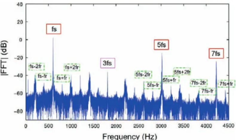
Experimental spectra in the case of healthy and faulty bearings are analyzed in this section in order to validate the theoretical spectral signatures defined inSection 2.2.1. The analysis is presented on current signals at 12,000 rpm where the current supply frequency is 600 Hz, but similar observations can be made on other speeds. The studied machine in this paper has 3 pole pairs which implies fr¼ 200 Hz at 12,000 rpm. According to the bearing characteristics (Nb¼ 8; Db¼
6.75 mm; Dc¼ 28.5 mm; θ ¼ 171), the cage fault frequency is fc¼ 77 Hz.Fig. 4shows the stator current spectrum in the case
of a healthy bearing.
It can be seen inFig. 4that harmonics in the current spectrum at fs, 5fs, and 7fscorresponding to the ð6k7 1Þfsfamily are
present. Moreover, harmonics can be observed at fs7nfr, 5fs7nfr, and 7fs7nfr. It seems to be part of the nfosc7ð6k 7 1Þfs
harmonic family with a speed oscillation at the rotor mechanical frequency fr. Since fs¼ 3fr, this harmonic family is
considered as the kfrharmonic family in the following.
Fig. 5shows the stator current spectrum in the case of a faulty bearing (close to its death). This spectrum (red plain line) is drawn on the top of the healthy spectrum presented inFig. 4(blue line) in order to enlighten the differences between the two.
As expected inSection 2.2.1, an increase is observed at fs7fc¼ 600 7 77 Hz: þ 5.3 dB at fs% fc and þ 9.5 dB at fsþ fc.
This increase is explained by the fact that the bearing degradation includes a broken cage. Increases are also observed on the spectrum for the kfr¼ k ! 200Hz harmonics: þ8.6 dB at fs% frand þ8.5 dB at fsþ fr along with increases at fsþ 3fr,
fsþ 5fr, 5fs, 5fs7frand 5fs% 5fr. This could be explained by the appearance of a speed modulation caused by the misplacing
of the grease in the rolling element. Moreover, this frequency can be seen as a multiple of the rotation frequency since it is Fig. 3. Example of stator current I1 on phase 1 generated by the PWM.
the case for the fundamental stator current frequency. Consequently, the proposed approach is focused on the components at kfras they seem to present the best sensitivity to the investigated bearing defaults.
2.3. Energy-based indicator
To compare the performance of the proposed method, a reference energy-based indicator is used. It is based on the classic approach of tracking spectral energy in specific frequency bands linked to bearing fault as described in[23]. For each recording, the stator current spectrum is computed using the FFT algorithm. The energy-based indicator E is then computed as the sum of the energy for the kfrharmonic family. A tolerance 7 Δf is added around the frequencies kfrin order to be
robust to potential shifts of considered frequencies. The algorithm is presented inFig. 6.
Fig. 5. Stator current spectrum in faulty (red plain line) and healthy (blue line) cases at 12,000 rpm. (For interpretation of the references to color in this figure caption, the reader is referred to the web version of this paper.)
Fig. 6. Energy-based indicator computation.
2.4. Statistic-based indicator 2.4.1. Stator current processing
In the proposed method, the spectrum stator current signal is computed using Welch's periodogram method[24]. This processing technique is an extension of Bartlett's averaging periodogram estimating the power spectrum of a signal as the average of the power spectra computed on subsegment of this signal. Welch's method adds overlapping between the different subsegment and windowing of the subsegment in order to reduce side effect. Let x(n) be a signal of length nsigand
w(n) be a window function. Considering subsegments of length L with 50% overlap, Welch periodogram Pwis the average of
the periodograms Picomputed on the K ¼ N=ð2Lþ1Þ subsegments and expressed as
Pw¼ 1 K ∑ K % 1 i ¼ 0 Pi ð4Þ
with Pibeing the periodogram computed on the ith subsegment as
Pi¼ & &∑L % 1 n ¼ 0w nð Þx n þiL2 " #e% jnω& & 2 ∑L % 1 n ¼ 0jwðnÞj 2 ð5Þ
The advantage of this method is to reduce power spectrum variance. According to[25], the variance estimation of the Welch periodogram Pw(assuming 50% overlap) can be expressed as
Var Pð wÞ C 9 16 L NP 2 x ð6Þ
with N being the total length of the signal, L the length of the subsegments and Pxthe power spectrum of the signal. The
analysis of Eq.(6)shows that the shorter the ratio of L=N is, the shorter the variance is. This means that a high number of subsegments (with a constant overlap) decrease the variance of the spectrum and so L has to be chosen short compared to N. In the same time, the frequency resolution depends only on the length L so a too short L implies a poor frequency resolution and increases the spectrum bias. Consequently, a compromise between L and N is to be found. This question is discussed inSection 3.2.
The next step is the statistical processing of the periodogram Pwin order to center and to reduce it. The spectral power in
dB at the frequency fi, taking values within ( % 1; þ 1½, is considered as a random variable following a normal distribution
N ðμi; siÞ over the recordings and noted P^wðfiÞ ¼ 20 logðPwðfiÞÞ. The centering of the random variable is calculated by
subtracting its mean μi. The variable ^PwðfiÞ % μiis then centered around 0. The operation of reduction is done by dividing
the centered variable by the standard deviation si. This operation can be seen as a normalization step. The mean and the
standard deviation of ^PwðfiÞ are computed on the first nref recordings in order to constitute a reference of the ^PwðfiÞ
distribution according to Eqs.(7) and (8) where E½X( denotes the expected value of X (here the average). μi¼ ∑ nref j ¼ 1 ^ Pw ðjÞ ðfiÞ nref ð7Þ si¼ ffiffiffiffiffiffiffiffiffiffiffiffiffiffiffiffiffiffiffiffiffiffiffiffiffiffiffiffiffiffiffiffi E½ð ^PwðfiÞ % μiÞ2( q ð8Þ For each frequency fi, the centered reduced spectrum PCRis then computed on every recording as the difference between the
current spectrum ^PwðfiÞ and the reference average μidivided by the standard deviation siaccording to
PCR fi
"
# ¼P^wðfiÞ % μi
si
ð9Þ Thus, PCRhas the same average μ ¼ 0 and standard deviation s ¼ 1 for each frequency bin. Spectral variations are easier to
detect as spectrum values are normalized and a statistical meaning can be associated to them. The operation performed to center and reduce spectral content can be assimilated to a Student t-test performed on each frequency bin evaluating how close is the spectral value from the reference distribution. The null hypothesis H0is that the considered sample is part of the
reference distribution and the hypothesis H1is that it is part of a different distribution. So, if the reference is taken on the
healthy working of the machine, it can be considered as a reference of the healthy behavior of the machine. If the hypothesis
H0is accepted, the sample is considered as “healthy”. If rejected, the sample is then considered as “faulty”. The choice of the
threshold λ to differentiate healthy and faulty cases can then be chosen according to the t-test table to differentiate H0and
H1, depending on the number of recordings used to build the reference which determines the degrees of freedom (dof).
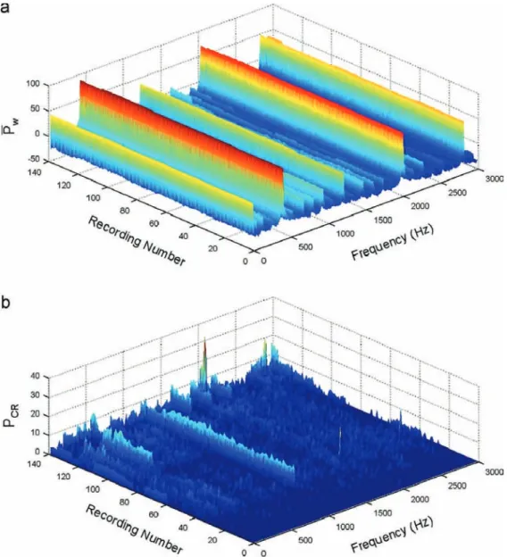
Fig. 7shows examples of a periodogram before (a) and after (b) being centered and reduced at 8000 rpm (campaign 1). The reference was computed on nref¼ 15 recordings (dof ¼ 14). According the Student t-test table[26], if a value is greater
than λ ¼ 2:98, it has a probability p¼0.01 to be part of healthy distribution, which means 99% chance to be part of another distribution that is considered as faulty. Only components greater than λ are shown inFig. 7b.
Fig. 7 shows that although no evident change appears in the spectral representation (a), the centered reduced representation (b) shows that the stator current spectrum moves away from the reference over time, which seems to match with the bearing deterioration. According toTable 1, the bearing has been changed after the 33rd recording in the
present case (campaign 1, 8000 rpm). It can indeed be seen inFig. 7b that there are only a very few components greater than λ¼ 2:98 till recording 33 whereas there are a lot of them after. Moreover, the values of these components seem to increase over the time at certain frequencies along with the bearing degradation. The proposed representation seems therefore well suited to monitor bearing degradations.
2.4.2. Indicator construction
According to the analysis inSection 2.2.2, it is decided to monitor the kfrharmonic family. The statistic-based indicator S
is computed in the following way. For each recording r, the Welch's periodogram Pw(f) of the stator current is computed. The
first nrefperiodograms are stored in order to compute the reference averages and standard deviations for each frequency.
The number nrefmust be large enough to consider the distribution by following a normal law and to correctly estimate its
mean and its standard deviation. This point can be easily confirmed by applying the Shapiro–Wilk test[27]. In practice, nref
must not be less than 15. Once the reference has been built, the next periodograms are centered and reduced as described in Section 2.4.1. The indicator is calculated as the sum of the centered reduced spectrum PCR(f) amplitude around the
frequencies kfrwith a tolerance 7 Δf according to
S rð Þ ¼∑
k
PCRðkfr7Δf Þ
nbins
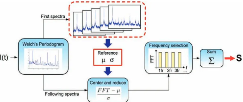
ð10Þ It is normalized by the number of frequency bins nbinsused in the calculation. The principle of the method is depicted in
Fig. 8andAlgorithm 1gives the computation procedure.
Algorithm 1. Statistical-based indicator. for eachrecording r do
^
Pw’20 logðFFTWelchðiðtÞÞÞ
if r r nref then Ptmp’½Ptmp;P^w( else if r ¼ nrefþ 1 then μ’∑Ptmpn ref s’ ffiffiffiffiffiffiffiffiffiffiffiffiffiffiffiffiffiffiffiffiffiffiffiffiffiffiffi E½ðPtmp% μÞ2( q end if PCR’ ^ Pw% μ s S¼ 0 for f ’kfrdo S’Sþ∑f þ Δff % ΔfPCR end for return S end if end for 2.4.3. Method relevance
Monitoring current spectral content can be difficult since current measures can be noisy. This noise might be due to the acquisition system, connectors, digital conversion or interferences with other electrical devices. It impacts that the current spectrum and the noise will also be found on spectral measures. As a result, harmonic amplitudes are not exactly constant and might fluctuate a bit. In this context, bearing fault detection based on spectral signatures may lead to false alarms due to noise. Using the Welch peridogram to assess spectral content will help minimizing this noise and so to decrease the number of possible false alarms. The integration of several spectra over time will indeed filter noise. Meanwhile, too much integration may also filter spectral increases due to bearing defects. A compromise is to be found through the choice of the number of windows used to compute the Welch spectrum. This point is addressed inSection 3.2.
Another point that might be difficult to address is the choice of a threshold to differentiate healthy and faulty functioning. The threshold choice depends on the harmonic amplitude and its variation range which often leads to an empirical threshold definition. To center and reduce the current spectrum allow us to have the same amplitude and the same standard deviation for all spectral components at the reference working conditions. This operation can be assimilated to a Student t-test and the threshold for abnormal functioning can be statistically defined using the Student table. All spectral components have the same threshold. Moreover, the visual representation is easier to analyze than the classic time– frequency representation since all components vary within the same range: the higher the value is, the further from the healthy reference the component is. So, a high value is likely to be a fault signature (if the reference is taken on healthy signals). On the contrary, it is sometimes not easy to appreciate harmonics variations on the classic time–frequency representation since variations on low amplitude harmonics might be visually attenuated due to high amplitude harmonics. Last, the inter- and intra-variability of electrical machines makes bearing fault detection system hardly reproducible since all parameters are proper to a specific machine and cannot be used on another one. The interest in building a healthy reference during the normal functioning of the machine is to have a picture of the machine current spectral content under healthy conditions. Then, the center and reduce operation normalizes the next spectrum to this healthy reference. Since the detection threshold is statistically defined and data are normalized, the same threshold can be used from one machine to another.
3. Results
3.1. Performance evaluation metrics
The performance of the energy-based and the statistic-based indicators is evaluated on data from campaigns 1 and 2. Campaign 1 is used as a training dataset in order to optimize the different parameters of the methods. These optimized criteria are then evaluated on campaign 2 to test if they are reproducible with different bearings. The vibration indicators recorded during both campaigns are used as references to compare the performance of the different methods because they are traditionally used to monitor bearing state of health.
The correlation coefficient r between spectral indicators and vibration indicators is computed for both energy-based and statistically-based indicators to evaluate if they are evolved in the same way than the vibration indicators. The correlation coefficient measures the extent to which two variables are correlated. The absolute value of this coefficient varies between 0 and 1. The closer to 1 the absolute value is, the stronger the linear relationship between the two variables is. Correlation was chosen because the indicators have different natures so it was not possible to directly compare the values obtained.
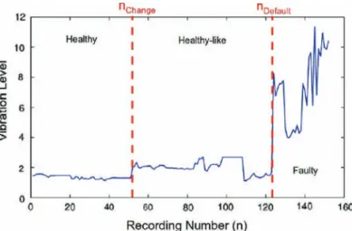
As explained inSection 2.1, the bearing degradation protocol used has been designed to guarantee a vibrational level very close to the healthy level for several hours of operation before the first signs of failure. So, when the bearing is changed, its behavior is still close to healthy for several hours and becomes really faulty only during the last working hours. The recording number when the bearing has been replaced by a faulty one has been marked during the campaign and is noted
nChange. Another marker is used to evaluate indicator performance when the vibration indicator starts highly reacting and
is noted nDefault. An illustration of these two markers is presented inFig. 9. The bearing is considered as “healthy” before
nChange, as “healthy-like” between nChangeand nDefaultand as “faulty” after nDefault.
Indicators are evaluated on their ability to detect faulty cases (after nDefault). Four metrics are then defined. The first one is
just a boolean saying if yes or no the indicator was able to detect the faulty behavior of the machine. It is noted Fault
Detection. The second metric is the false alarm rate FPratewhich is the ratio between the number of false detection (detection
before nDefault) and the number of healthy and healthy-like cases computed as
FPrate¼
Number of false detections
Total number of healthy and healthy%like cases ð11Þ
The third metric is the percentage of delay for the fault detection. It is computed as the difference between the time nDetection
when the fault is detected by the indicator for the first time and the marker nDefaulton the number of recordings elapsed
between nDefaultand the last recording nFinalwhen the bearings break according to
Delay ¼nDetection% nDefault nFinal% nDefault
ð12Þ The closer to 0 the FPrateand the delay are, the more accurate the detection is. The last metric is the indicator stability which
evaluates the quality of the detection continuity. It is computed as the number of correct detections between the first fault detection and the bearing break. It is expressed as
Stability ¼Number of correct detections nFinal% nDetection
ð13Þ The closer to 1 the stability, the more accurate the detection is.
The different indicators are labeled according to the recording numbers n. Since the recording time has been saved for each recording and data were recorded every hours, it is easily possible to deduce the time from the recording number.
3.2. Method optimization
The different indicators are computed on each 5 s recording. The frequency tolerance used was Δf ¼ 10 Hz. The kfr
frequencies were computed till k¼12 in order to have the same number of frequency bins at each speed and to restrain the indicator to frequencies lower than ð6 %1Þfs. The reference is computed on half the healthy recordings in order to keep the
other half to test the indicators on. In that way, a reference of the healthy working of the machine is built. Depending on the degree of freedom dof ¼ nref% 1, the threshold λ above which there is a probability p ¼ 0.01 to be part of the reference
healthy distribution is chosen in the Student table. This means that if a value is greater than λ, it has 99% chance not to be part of the healthy distribution so it can be considered as part of some “faulty” distribution. Only the components greater than λ are taken into account, the other components are forced to 0. When the statistic-based indicator S is greater than λ, then the bearing is considered as faulty. The detection threshold depends only on the number of recordings used to compute the reference. So, the same threshold can be used whatever the speed or the machine supposing the references has the same length.
It has been shown inSection 2.4through the analysis of Eq.(6)that a compromise is to be found for the choice of L the length of window used to compute the Welch periodogram. The length of this window determines the number of periodograms that are averaged to compute the spectrum and so its variance. Several ratios of L=N with N being the total length of the signal are tested in order to evaluate the impact of this criteria. The length N is kept to 5 s in order to have a better frequency resolution. The different ratio tested are f1;1
2; 1 4; 1 8; 1 10; 1
20g. An overlap of 50% is chosen as assumed in
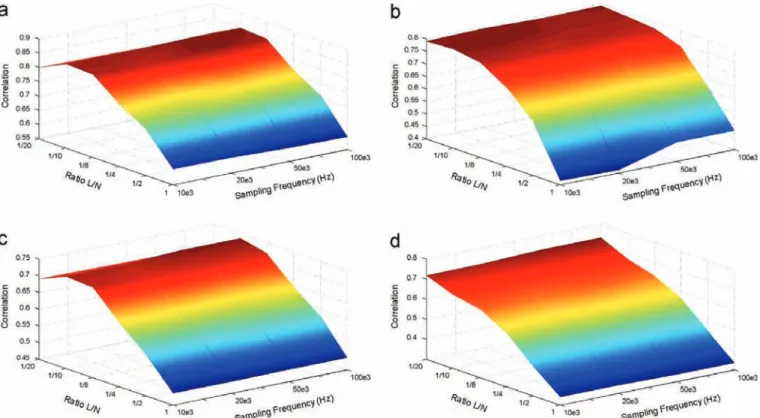
Section 2.4.1. In the same time, the influence of the sampling frequency is also evaluated as a 200 kHz sampling frequency that is not conceivable for on-line industrial applications. The current signal has been down-sampled to the following frequencies: {10, 20, 50, 100} kHz. The correlation coefficients between the statistic-based indicator and the vibration indicator for campaign 1 at the different speeds are presented inFig. 10.
It can be seen inFig. 10that the worst results are obtained when no averaging is done (L=N ¼ 1). In this case correlation is very low (r o 0:5) which means that the statistic-based indicator does not evolve like the vibration indicator. This is due to a high variance which makes difficult to differentiate variations that are statistically significant and those that are due to noise. Decreasing the ratio L=N increases the performance at all speeds and gives good correlation rates at around 0.75. This means that statistic-based indicators and vibration indicators evolve globally the same way. Decreasing L=N increases the number of windows used in the computation of Welch periodogram and decreases its variance as shown in Eq.(6). As the variance is low, the reference is less noisy and it is then easier to detect statistically significant variations. As expected,Fig. 10 shows that too much averaging attenuates variations due to bearing defect. Results start indeed decreasing for L=N ¼ 1
20 at
speeds 8000 and 12,000 rpm. The statistic-based indicator is not impacted by the sampling frequency. This was expected
Fig. 10. Correlation results of the statistic-based indicator for different window sizes and sampling frequencies at 8000 rpm (a), 10,000 rpm (b), 12,000 rpm (c) and 14,100 rpm (d).
because the monitored frequencies are low ( o5fs¼ 3525 Hz at 14,100 rpm) so a sampling frequency fe¼ 10 kHz is sufficient.
In the following, results are presented for a sampling frequency fe¼ 10 kHz with a ratio L=N ¼101 . The Welch window length
is L ¼ 5
10¼ 0:5 s and 10 ! 2 % 1 ¼ 19 spectra are used to compute the Welch periodogram with 50% overlap.
It is obvious from Fig. 10 that the sampling frequency has no influence on the performance of the statistic-based indicator. For a given ratio L=N, the correlation coefficient between the statistic-based indicator and the vibration one stays the same whatever the sampling frequency. This result was predictable since only harmonics lesser than 5fs(¼3525 Hz at
14,100 rpm) are monitored. The Shannon sampling theorem is verified even at the lowest sampling frequency of 10 kHz. Using a greater sampling frequency does not add useful information to the indicator. For this reason, the sampling frequency is set to 10 kHz in the following.
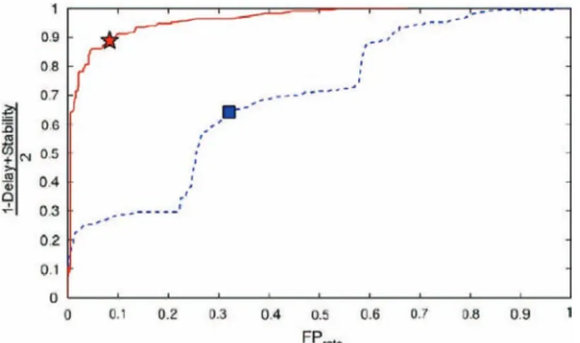
The choice of the detection threshold is an important issue. This threshold is empirically defined on campaign 1 for both indicators in order to minimize both the delay of detection and the false alarm rate while ensuring the bearing fault detection and maximizing the stability. The aim here is to study the robustness of the indicators to different speeds and their reproducibility. In this purpose, several threshold values have been evaluated on both energy-based and statistic-based indicator at the four different speeds for campaign 1. The results are plotted inFig. 11. It displays the average value between 1 %Delay and Stability (which can be seen as a compromise between a early detection and a stable detection) in function of the false alarm rate FPratefor each threshold value. The right part ofFig. 11corresponds to lower threshold values while the
left part corresponds to higher threshold values. This is coherent: increasing the threshold value will diminish the number of false alarms while decreasing also the number of correct of detection. Threshold values vary from %125 to % 75 dB for the energy-based indicator (dashed blue line) and from 0 to 5 for the statistic-based indicator (plain red line).
The optimal threshold value soptis defined fromFig. 11as the value minimizing false alarms and delay while maximizing
the stability of the indicator. Graphically, this value can be defined by the one corresponding to the closest point to the up-left corner. It is pictured as a red star for the statistic-based indicator and a blue box for the energy-based indicator inFig. 11. These values are sopt¼ % 106:5 dB for the energy-based indicator and sopt¼ 0:45 for the statistic-based one. The choice of a
threshold value for the statistic-based indicator is pretty obvious fromFig. 11as the red curve presents a clear elbow point. This can be explained because the statistic-based indicator is normalized and evolves in the same range whatever the speed. This point shows that the proposed indicator is robust to the different speeds. It is then possible to define a common threshold value for the different speed even it seems illusory to think of a universal threshold value. On the contrary, the shape of the blue curves shows three elbow points which indicate that it is difficult to define a common threshold value for the energy-based indicator. The three elbow points show that the threshold value depends on the speed for the energy based indicator. This point is confirmed when looking at the optimal threshold values at each speed for the energy based indicator. These values, presented inTable 2, are indeed a little distant from each other.
Fig. 11. Results of the bearing fault detection on campaign 1 in terms of false alarms, delay and stability with different threshold values for energy-based (dashed blue) and statistic-based indicators (plain red). The optimal points are pictured as a box and a star respectively. (For interpretation of the references to color in this figure caption, the reader is referred to the web version of this paper.)
Table 2
Optimized threshold for bearing fault detection on campaign 1 with the energy-based indicator.
Speed (rpm) Fault detection threshold (dB)
8000 % 112.9
10,000 % 106.2
12,000 % 101.5
In order to evaluate the robustness of the different indicators, the threshold values defined in this section (on campaign 1) are used on campaign 2 in the following.
3.3. Performance of the energy-based indicator
The energy-based indicator is computed on both campaigns for the four different speeds. The indicators obtained on campaign 1 are shown in Fig. 12and the ones obtained on campaign 2 inFig. 13. The vibration indicators are plotted in dotted red line in both figures. They are scaled in order to evolve in the same range as the energy-based indicator.
It can be seen inFigs. 12and13that the energy-based indicators have globally the same shape as the vibration indicators. They are nevertheless very noisy which might lead to false alarms and a lack of stability.Tables 3and4show the results of the energy-based indicators on campaigns 1 and 2 respectively. These values are obtained using the optimal threshold values defined inTable 2.
The first point showed byTable 3is that the bearing fault is detected in all cases. The analysis ofTable 3points out that the correlation results are average with an overall r¼0.58. It confirms the observation done in Fig. 12: the energy-based indicator shape is about the same as the vibration indicator one. The average value can be explained by the high variability of the indicator. The delay value is good with an overall 1.6% which means that the indicator is reacting at the same time than the vibration indicator. Meanwhile, the stability value is decent with almost 70%. It means that once the fault has been detected, it stays detected for 70% of the time which might make it difficult to differentiate from false alarms if the indicator is oscillating after the detection. The false alarm rate varies from 1.8% to 21.7%. The overall value is acceptable (FPrate¼ 10:9%) but still a little high which can be explained by the variability of the indicator. Except for the false alarms
rate, results are very stable with the speed which is a good point but this point is biased by the fact that they have been obtained with threshold values optimized for each speed.
The analysis ofTable 4shows that bearing fault is detected in all cases in campaign 2 with no delay (overall 0%) and a perfect stability (overall 100%) but the overall FPrate¼ 99:4% demonstrates that the threshold values are wrong. These values
have indeed been optimized for indicators on campaign 1 and are not suitable on campaign 2 since the energy-based indicator is always greater than the threshold value. In order to evaluate these indicators, the optimal threshold values for campaign 2 are computed the same way as described inSection 3.2. The results obtained with these new values are
Fig. 12. Energy-based indicators (plain blue line) and vibration indicators (dotted red line) obtained on campaign 1 at different speeds. (For interpretation of the references to color in this figure caption, the reader is referred to the web version of this paper.)
presented inTable 5. Concerning the correlation results, they are less stable than for campaign 1. These results are correct at speeds 8000 and 14,100 rpm (r¼0.59 and r¼0.71 respectively) but the correlation is very weak at 10,000 and especially at 12,000 rpm where there seems to be no correlation at all (r ¼ %0:49) between the energy-based and the vibration indicators.
The threshold values optimized on campaign 2 are presented inTable 5. Their values are very different from the one optimized on campaign 1 (displayed inTable 2) although both campaigns have been performed on the same machine with the same bearing ageing protocol. This point is a downside concerning the reproducibility of the energy-based indicator. Fig. 13. Energy-based indicators (plain blue line) and vibration indicators (dotted red line) obtained on campaign 2 at different speeds. (For interpretation of the references to color in this figure caption, the reader is referred to the web version of this paper.)
Table 3
Results of the energy-based indicator on campaign 1.
Speed (rpm) 8000 10,000 12,000 14,100 Overall
Detection Yes Yes Yes Yes Yes
Correlation 0.63 0.60 0.57 0.53 0.58
Delay (%) 3.5 0 0 2.9 1.6
Stability (%) 57.1 82.7 65.5 73.5 69.7
FPrate(%) 1.8 21.7 11.4 8.6 10.9
Table 4
Results of the energy-based indicator on campaign 2 with threshold optimized on campaign 1.
Speed (rpm) 8000 10,000 12,000 14,100 Overall
Detection Yes Yes Yes Yes Yes
Correlation 0.59 0.41 % 0.49 0.71 0.30
Delay (%) 0 0 0 0 0
Stability (%) 100 100 100 100 100
The bearing fault is detected in all cases but the threshold values have been optimized to do so. The correlation results are obviously unchanged from Table 4 since the correlation does depend not only on the threshold value but also on the indicator's shape. The delay is varying a lot from one speed to another. The delay is equal to 85% at 8000 rpm while there is none at 14 100 rpm. It is interesting to note that the stability results evolve the opposite way than the delay results. It can indeed be seen inTable 5that the later the fault is detected, the more stable the detection is. This can be explained by the strong variations of the indicator. This fact points out the need to find a compromise between an early detection and a stable detection for the energy-based indicator. At last, the number of false alarms remains low with an overall FPrate¼ 5:8%.
3.4. Performance of the statistic-based indicator
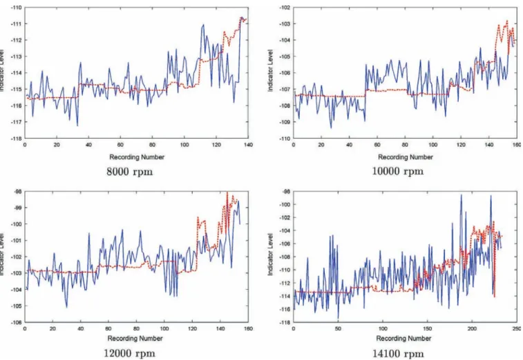
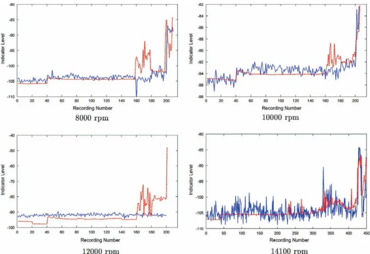
The statistic-based indicator is computed on both campaigns for the four different speeds. The indicators obtained on campaign 1 are shown in Fig. 14and the ones obtained on campaign 2 inFig. 15. The vibration indicators are plotted in dotted red line in both figures. They are scaled in order to evolve in the same range as the statistic-based indicator.
Figs. 14and15show that the statistic-based indicators evolve in the same way as the vibration indicators. Moreover they present a clear distinction between the healthy (on the left) and the faulty (on the right) recordings and their levels are
Table 5
Results of the energy-based indicator on campaign 2 with threshold optimized on campaign 2.
Speed (rpm) 8000 10,000 12,000 14,100 Overall
Threshold (dB) % 100.0 % 92.7 % 90.9 % 101.1 % 96.2
Detection Yes Yes Yes Yes Yes
Correlation 0.59 0.41 % 0.49 0.71 0.30
Delay (%) 85.2 40.5 17.9 0 35.9
Stability (%) 100 60.0 18.7 29.3 52.0
FPrate(%) 0 8.6 11.2 3.3 5.8
Fig. 14. Statistic-based indicators (plain blue line) and vibration indicators (dotted red line) obtained on campaign 1 at different speeds. (For interpretation of the references to color in this figure caption, the reader is referred to the web version of this paper.)
globally stable. The fault detection results of the statistic-based indicators are respectively presented inTables 6and7. These values have been obtained using the optimal threshold value sopt¼ 0:45 defined inSection 3.2.
The analysis ofTable 6shows that correlation is strong between statistic-based and vibration indicators on campaign 1 with an overall correlation r¼0.79. This point confirms that the statistic-based and the vibration indicators evolve the same way as observed in Fig. 14. Bearing faults are detected in all cases. The delay is very short ( r 3:4%) except at speed Fig. 15. Statistic-based indicators (plain blue line) and vibration indicators (dotted red line) obtained on campaign 2 at different speeds. (For interpretation of the references to color in this figure caption, the reader is referred to the web version of this paper.)
Table 6
Results of the statistic-based indicator on campaign 1.
Speed (rpm) 8000 10,000 12,000 14,100 Overall
Detection Yes Yes Yes Yes Yes
Correlation 0.85 0.80 0.84 0.67 0.79
Delay (%) 0 51.7 3.4 2.8 14.5
Stability (%) 86.2 100 57.1 100 85.8
FPrate(%) 0 3.1 0 8.1 2.8
Table 7
Results of the statistic-based indicator on campaign 2.
Speed (rpm) 8000 10,000 12,000 14,100 Overall
Detection Yes Yes Yes Yes Yes
Correlation 0.77 0.69 0.50 0.84 0.70
Delay (%) 20.8 40.4 2.5 0 15.9
Stability (%) 81.5 100 65.8 62.9 78.6
10,000 rpm. In this particular case, the delay is quite important (Delay ¼ 51:7%) but the detection remains very stable (Stability ¼ 100%) which means that even if the statistic-based indicator reacts later than the vibration one, once the default has been detected, the detection is sure. On the whole, the statistic-based indicator remains very stable with an overall stability of 85.8%. The stability is a bit low at speed 12,000 rpm with only 57.1% but this can be explained by the particular indicator shape at this speed. The statistic-based indicator reacts a first time, goes down and then reacts a second time which explains that the fault is not detected during the down part. Nevertheless, the vibration indicator reacts the same way as attested by the strong correlation coefficient r¼0.84. At last, the false alarm rate is very low with an overall FPrates¼ 2:8%.
The fact that the threshold value has been optimized on this campaign may temper these very good results. Nevertheless, it is interesting to note that all these results have been obtained with the same threshold value.
The analysis of the results obtained on campaign 2 and presented inTable 7is quite similar to observations done on campaign 1. Bearing faults are detected at all speeds. The correlation results are a bit lower than the ones obtained for campaign 1. This can be explained by the fact that the statistic-based indicator reacts later than the vibration indicator at speeds 8000 and 10,000 rpm. It can also be explained by the average correlation coefficient r¼ 0.50 at 12,000 rpm showing the fact that the statistic-based indicator moderately reacts in this case. The overall correlation result is however good with
r¼0.70. As already mentioned, the indicator reacts lately at 8000 rpm and 10,000 rpm which explains the delay results at
these speeds, even if they remain very low ( o 3%) for the other speeds. The overall stability is very good with 78.6%. The stability is higher with the delay which is a good point. It means that when the fault is detected later, the detection is surer. It enlightens the need to find a compromise between a fast and a sure fault detection. The false alarm rate remains low at all speed with an overall FPrate¼ 5:6%. It is important to note that the overall performance is very close to the ones obtained on
campaign 1 although they have been obtained using the same threshold value as in campaign 1. 4. Discussion
Bearing faults are detected at each speed for both campaign either by energy-based or statistic-based indicators. The comparison between the results obtained with the energy-based indicator (Section 3.3) and with the statistic-based indicator (Section 3.4) shows that the use of the statistic-based indicator leads to a more accurate detection of bearing faults. Table 8resumes the overall results on campaigns 1 and 2 for both indicators. The results presented inTable 8are the average of the ones presented inTables 3and5for the energy-based indicator and the average of the ones presented inTables 6 and7for the statistic-based indicator.
The correlation coefficient is stronger for the statistic-based indicator than for the energy-based one. This point confirms that the shape of the statistic-based indicators is closer to the one of the vibration indicators as it can be seen inFigs. 14 and15. Concerning the delay of detection,Table 8seems to indicate is equivalent for both indicators. Nevertheless, a look at the detailed results shows that the delay fluctuates more for the energy-based indicator (1.6% on campaign 1 and 30.4% on campaign 2) than for the statistic-based indicator (14.5% on campaign 1 and 15.9% on campaign 2). Concerning the campaign 1, the better delay results obtained with the energy-based indicator must be weighted against the stability of 69.7% while the statistic-based indicator has a stability of 85.8%. So, even if the statistic-based fault detection is a little later (Delay ¼ 14:5%) the energy-based fault detection, it is compensated by very good stability which makes the detection surer. In the case of campaign 2, the statistic-based detection presents better delay and stability results.Table 8shows that the statistic-based indicator is more stable than the based indicator. This point was predictable because the energy-based indicator is noisier according toFigs. 12and13. Moreover, a detection delay of about 15% represents about 3 h and a half when the bearing stays in a faulty state for about 25 h. Consequently, the delay of detection is not a critical issue because the bearing degradation evolves quite slowly. The good stability results of the statistic-based indicator compensate for its short delay of detection. The number of false alarms is twice smaller for the statistic-based indicator than for the energy-based indicator (4.2% against 8.3%) which can be explained by the fact that the statistic-based indicator shows less variability than the energy-based indicator.
An important point is the fact that all the results of the statistic-based indicator are obtained with the same threshold value whereas the threshold values used for the energy-based indicator are optimized for each speed and campaign. Moreover results of the statistic-based indicator are very stable from campaigns 1 to 2 with the same threshold when results of the energy-based detection fluctuate a lot between the 2 campaigns. A major advantage of the statistic-based indicator is that it is a normalized indicator. This is an important point as it allows us to use the same threshold value at all speeds in contrast to the energy based indicator where the threshold has to be tuned for every speed. Moreover, the differences between both campaigns on the frequency content (threshold values are very different for the energy-based indicator) and
Table 8
Overall results of the energy-based and the statistic-based indicators on both campaigns.
Indicator Detection Correlation Delay (%) Stability (%) FPrate(%)
Energy-based Yes 0.44 18.7 60.8 8.3
on the vibratory signals (vibratory levels at the bearing break is different in the 2 campaigns) whereas they have been performed on the same machine with the exact same ageing process, points out the need of normalized detection methods. It is demonstrated inSection 3.3that it is not possible to use the same threshold values from one campaign to another for the energy-based indicator whereas the statistic-based indicator reaches very good performance whatever the campaign or the speed with a unique threshold value.
The statistic-based indicator presents a short delay of detection compared to the vibration indicator. This can be seen in particular inFig. 14at 10,000 rpm and inFig. 15at speeds 8000 and 10,000 rpm where the vibration indicator starts reacting earlier than the statistic-based one. It seems to be due to the frequency content of the current signal since this is also the case for the energy-based indicator. An explanation might be that the early burst of the vibration indicator could be due to high frequencies. The vibration indicator is indeed computed in a frequency range from 1 to 19 kHz (as specified in Section 2.1) while the statistic-based indicator is computed on frequencies less than 4 kHz. Nevertheless, computing the statistic-based indicator on the same frequency range than the vibration one would impose a high sampling frequency (at least 40 kHz) which is not a good point for the implementability of the proposed method. A higher sampling frequency would mean more memory needed to store the data as well as a higher computation cost. In the same time, the delay of detection of the statistic-based indicator is not very important (overall Delay ¼ 15:2%). Even if the statistic-based indicator reacts a few recordings after the vibration indicator, the bearing fault is detected soon enough before the bearing breaks (about 30 recordings before which is about 20 h of working). Moreover, this detection delay is compensated by a very good stability and a low false alarm rate which implies that once the fault is detected, it is detected for good.
The performance of the statistic-based indicator could be improved with the computation of a longer reference. The reference is computed here on about 20 recordings (less than 15 h of working) so it might not be rich enough to compute complete reference. For example, it can be seen inFig. 14at 14,100 rpm that some detections happen during the beginning of the indicator while the bearing is still healthy. This mean that some behavior of the healthy bearing is not taken into account during the reference computation. This will lead to false alarms. The computation of a longer reference could lead to a better differentiation between healthy and faulty bearings and a decrease of the false alarms number. It has been decided here to keep a short reference in order to keep some healthy recordings to evaluate the proposed indicators. Nevertheless, the computation needs to be done on a constant operating point and the detection is processed at this operating point. A transient (at variable speed) will be seen as a change of behavior by the statistic-based indicator and considered as a fault because the frequency content will change with the operating point.
5. Conclusion
An original method for bearing fault detection in permanent magnet synchronous machine is designed and evaluated in this paper. This method statistically processes the stator current spectrum in order to detect changes from a reference frequency content. The stator current spectrum is computed according to Welch's method in order to minimize its variance. A reference is then built on a set of spectra by calculating the mean and the standard variation for each frequency bin. As this reference is built during the healthy working of the machine, it is considered as a “healthy” reference. The following spectra are centered and reduced according to this reference. The centered reduced spectrum gives an indication on how much the stator current spectrum changed from the reference, similar to a Student t-test. An indicator is then computed by summing the centered reduced spectrum contributions on the kfrfrequency family as it has been found to be the most reacting family
to bearing faults.
The proposed method is optimized and evaluated on 2 different test campaigns for 4 different speeds with a standard-ized bearing ageing process. As compared to the vibration indicator, the statistic-based indicator shows a strong correlation (r¼ 0.74) and provides with an accurate estimation of the bearing state of health. It demonstrates a good overall performance with a detection delay of 15.2%, a stability of 82.2% and only 4.2% of false alarms according to the evaluation metrics. Comparison of these results with those obtained with a traditional energy-based indicator revealed that the statistic-based indicator is closer to the vibration indicator. It is more stable than the energy-based indicator and results in twice less false alarms. Moreover, the better performance of the statistic-based indicator is emphasized by the fact that it is obtained with the same threshold value for all campaigns and speeds while the energy-based detection threshold has to be optimized on every campaign and every speed. The rigorous performance evaluation metrics used in this study lead to the conclusion that the statistic-based indicator achieves a more accurate bearing fault detection as it is more stable and more reproducible. The impossibility of using the same threshold on the energy-based indicator from one campaign to another enlightens the need of normalized indicator such as provided by the proposed method.
In machine diagnostic, existing work has validated energy-based indicators for bearing fault detection but have most of the time evaluated their technique on only one machine. The present work shows that bearing faults were hardly reproducible from one machine to another. It highlights the need to develop normalized indicators whose performance is reproducible. Further work should explore adjustment of the proposed method to induction machines. The slipping phenomena specific to this kind of machine should provide with an interesting problematic the proposed method will have to adapt to. In a more general way, the question of how to adapt this technique to applications with variable operating points is still very challenging.
Acknowledgments
This work is part of the French national project PREMEP[21](PRojEt Moteur Electronique de Pilotage), labeled by the Aerospace Valley cluster and involving the LAPLACE and Airbus suppliers such as Technofan, Liebherr Aerospace, CIRTEM, DELTY and ADN. It was founded by the Fond Unique d'Investissement, and the Aquitaine and Midi Pyrénées regions. References
[1]P.J. Tavner, Review of condition monitoring of rotating electrical machines, IET Electr. Power Appl. 2 (4) (2008) 215–247.
[2] S. Jeevanand, B. Singh, B. Panigrahi, V. Negi, State of art on condition monitoring of induction motors, in: Proceedings of the Joint International Conference on Power Electronics, Drives and Energy Systems (PEDES), 2011, pp. 1–7.
[3]S. McInerny, Y. Dai, Basic vibration signal processing for bearing fault detection, IEEE Trans. Educ. 46 (1) (2003) 149–156.
[4] A. Sadoughi, M. Ebrahimi, E. Razaei, A new approach for induction motor broken bar diagnosis by using vibration spectrum, in: Proceedings of the International Joint Conference SICE-ICASE, 2006.
[5] W. Zhaoxia, L. Fen, Y. Shujuan, W. Bin, Motor fault diagnosis based on the vibration signal testing and analysis, in: Proceedings of the 3rd International Symposium of Intelligent Information Technology Application, Nanchang, China, 2009, pp. 433–436.
[6]J. Antoni, R. Randall, The spectral kurtosis: application to the vibratory surveillance and diagnostics of rotating machines, Mech. Syst. Signal Process. 20 (2) (2006) 308–331.
[7]J. Chebil, G. Noel, M. Mesbah, M. Deriche, Wavelet decomposition for the detection and diagnosis of faults in rolling element bearings, Jordan J. Mech. Ind. Eng. 3 (4) (2009) 260–267.
[8] S. Ai, H. Li, Y. Zhang, Condition monitoring for bearing using envelope spectrum of EEMD, in: Proceedings of the International Conference on Measuring Technology and Mechatronics Automation 2009, ICMTMA'09, vol. 1, 2009, pp. 190–193.
[9] V. Vrabie, P. Granjon, C.-S. Maroni, B. Leprettre, Application of spectral kurtosis to bearing fault detection in induction motors, in: Proceedings of the 5th International Conference on Acoustical and Vibratory Surveillance Methods and Diagnostic Techniques, Senlis, France, 2004.
[10] A. Hazan, M. Verleysen, M. Cottrell, J. Lacaille, Probabilistic outlier detection in vibration spectra with small learning dataset, in: Proceedings of the International Conference Surveillance, vol. 6, 2011.
[11] H. Henao, H. Razik, G.-A. Capolino, Analytical approach of the stator current frequency harmonics computation for detection of induction machine rotor faults, IEEE Trans. Ind. Appl. 41 (3) (2005) 801–807.
[12] M. Blodt, M. Chabert, J. Regnier, J. Faucher, Mechanical load fault detection in induction motors by stator current time-frequency analysis, IEEE Trans. Ind. Appl. 42 (6) (2006) 1454–1463.
[13] B. Trajin, J. Regnier, J. Faucher, Comparison between vibration and stator current analysis for the detection of bearing faults in asynchronous drives, IET Electr. Power Appl. 4 (2) (2010) 90–100.
[14] W. Zhou, T. Habetler, R. Harley, Stator current-based bearing fault detection techniques: a general review, in: Proceedings of the IEEE International Symposium on Diagnostics for Electric Machines, Power Electronics and Drives, Cracow, Poland, 2007, pp. 7–10.
[15] E.H. El Bouchikhi, V. Choqueuse, M. Benbouzid, J.F. Charpentier, Induction machine fault detection enhancement using a stator current high resolution spectrum, in: Proceedings of the 38th Conference on IEEE Industrial Electronics Society, IECON'12, Montreal, Canada, 2012.
[16] J. Rosero, J. Romeral, J. Cusido, J. Ortega, A. Garcia, Fault detection of eccentricity and bearing damage in a PMSM by means of wavelet transforms decomposition of the stator current, in: Proceedings of the 23rd IEEE Applied Power Electronics Conference and Exposition, Austin (TX), USA, 2008, pp. 111–116.
[17] Z. Obeid, A. Picot, S. Poignant, J. Regnier, O. Darnis, P. Maussion, Experimental comparison between diagnostic indicators for bearing fault detection in synchronous machine by spectral kurtosis and energy analysis, in: Proceedings of the 38th Conference on IEEE Industrial Electronics Society, Montreal, Canada, 2012.
[18] A. Picot, Z. Obeid, S. Poignant, J. Regnier, O. Darnis, P. Maussion, Bearing fault detection in synchronous machine based on the statistical analysis of stator current, in: Proceedings of the 38th Conference on IEEE Industrial Electronics Society, IECON'12, Montreal, Canada, 2012.
[19] E. Fournier, A. Picot, J. Regnier, M. Tientcheu Yamdeu, J. Andrejak, P. Maussion, On the use of spectral kurtosis for diagnosis of electrical machines, in: Proceedings of 9th IEEE International Symposium on Diagnostics for Electric Machines, Power Electronics and Drives (SDEMPED), Valencia, Spain, 2013, pp. 77–84.
[20] R. Randall, J. Antoni, Rolling element bearing diagnostics—a tutorial, Mech. Syst. Signal Process. 25 (2011) 485–520.
[21] O. Darnis, S. Poignant, K. Benmachou, M. Couderc, Z. Obeid, M. Nguyen, J. Régnier, D. Malec, D. Mary, P. Maussion, PREMEP, a research project on electric motor optimization, diagnostic and power electronics for aeronautical applications, in: Proceedings of the International Conference on Recent Advances in Aerospace Actuation Systems and Components, Toulouse, France, 2010, pp. 127–132.
[22] J. Stack, T. Habetler, R. Harley, Fault classification and fault signature production for rolling element bearings in electric machines, IEEE Trans. Ind. Appl. 40 (3) (2004) 735–739.
[23] Z. Obeid, S. Poignant, J. Régnier, P. Maussion, Stator current based indicators for bearing fault detection in synchronous machine by statistical frequency selection, in: Proceedings of the 37th Conference on IEEE Industrial Electronics Society, Melbourne, Australia, 2011, pp. 2036–2041. [24] P. Welch, The use of fast Fourier transform for the estimation of power spectra: a method based on time averaging over short, modified periodograms,
IEEE Trans. Audio Electroacoust. 15 (1967) 70–73.
[25] M.H. Hayes, Statistical Digital Signal Processing and Modeling, John Wiley and Sons, New York, 1996. [26] S.S. Wilks, Mathematical Statistics, J. Wiley and Sons, New York–London, 1962.
[27] S. Shapiro, M. Wilk, An analysis of variance test for normality (complete samples), Biometrika 52 (3) (1965) 591–611. –