To link to this article
: DOI: 10.1111/str.12054
http://onlinelibrary.wiley.com/doi/10.1111/str.12054/abstract
This is an author-deposited version published in:
http://oatao.univ-toulouse.fr/
Eprints ID: 10589
To cite this version:
Amiot, Fabien and Bornert, Michel and Doumalin, Pascal and Dupré,
Jean-Christophe and Fazzini, Marina and Orteu, Jean-José and Poilane,
Christophe and Robert, Laurent and Rotinat, René and Toussaint, Eveline
and Wattrisse, Bertrand and Wienin, Jean-Samuel Assessment of digital
image correlation measurement accuracy in the ultimate error regime:
main results of a collaborative benchmark. (2013) Strain, vol. 49 (n°6).
pp. 483-496. ISSN 1475-1305
O
pen
A
rchive
T
oulouse
A
rchive
O
uverte (
OATAO
)
OATAO is an open access repository that collects the work of Toulouse researchers and
makes it freely available over the web where possible.
Any correspondence concerning this service should be sent to the repository
administrator:
[email protected]
Assessment of Digital Image Correlation Measurement
Accuracy in the Ultimate Error Regime: Main Results of
a Collaborative Benchmark
F. Amiot
*, M. Bornert , P. Doumalin , J. -C. Dupré , M. Fazzini , J. -J. Orteu , C. Poilâne
, L. Robert ,
R. Rotinat
§§, E. Toussaint
¶¶, B. Wattrisse
*0and J. S. Wienin
***FEMTO-ST, CNRS-UMR 6174, UFC/ENSMM/UTBM, Besançon, France
†Laboratoire Navier (UMR 8205), CNRS, ENPC, IFSTTAR, Université Paris-Est, Marne-la-Vallée, France ‡Institut P’, UPR 3346 CNRS, Université de Poitiers, SP2MI, Futuroscope Chasseneuil, France
§INP/ENIT, LGP EA 1905, Université de Toulouse, Tarbes, France
¶Mines Albi, INSA, UPS, ISAE; ICA (Institut Clément Ader), Université de Toulouse, Campus Jarlard, F-81013, Albi Cedex 09, France ††CIMAP, UMR6252, Université de Caen Basse-Normandie, CNRS, CEA, ENSICAEN, Caen, France
‡‡LAUM, UMR 6613, CNRS, Université du Maine, Le Mans, France §§LMPF, Arts et Metiers ParisTech, Châlons en Champagne, France
¶¶Institut Pascal, UMR6602, Université Blaise Pascal – IFMA, Aubière, France
*0Laboratoire de Mécanique et Génie Civil, UMR CNRS 5508, Université Montpellier 2, Montpellier, France **École des Mines d’Alès, Alès, France
ABSTRACT: We report on the main results of a collaborative work devoted to the study of the uncertainties associated with Digital image correlation techniques (DIC). More specifically, the dependence of displacement measurement uncertainties with both image characteristics and DIC parameters is emphasised. A previous work [Bornert et al. (2009) Assessment of digital image correlation measurement errors: methodology and results. Exp. Mech. 49, 353–370] dedicated to situations with spatially fluctuating displacement fields demonstrated the existence of an ‘ultimate error’ regime, insensitive to the mismatch between the shape function and the real displacement field. The present work is focused on this ultimate error. To ensure that there is no mismatch error, synthetic images of in-plane rigid body translation have been analysed. Several DIC softwares developed by or in use in the French community have been used to explore the effects of a large number of settings. The discrepancies between DIC evaluated displacements and prescribed ones have been statistically analysed in terms of random errors and systematic bias, in correlation with the fractional part τof the displacement component expressed in pixels. Main results are as follows: (i) bias amplitude is almost always insensitive to subset size, (ii) standard deviation of random error increases with noise level and decreases with subset size and (iii) DIC formulations can be split up into two main families regarding bias sensitivity to noise. For the first one, bias amplitude increases with noise while it remains nearly constant for the second one. In addition, for the first family, a strong dependence of random error with τ is observed for noisy images.
KEY WORDS: Digital Image Correlation (DIC), image matching, random error, synthetic images, systematic error
Introduction
Digital image correlation (DIC) is a full-field kinematic measurement technique, which has recently become one of the most standard tools in the field of experimental solid mechanics [1, 2]. Among the optical contactless full-field techniques [3, 4] including interferometric methods (e.g. speckle or grating interferometry, holography interferometry) or non-interferometric methods such as the grid method, the DIC method has become very attractive and is now commonly used for measurements of surface deformation. The rapid diffusion of this technique can mostly be explained by operability, flexibility and (apparent) ease of use in comparison with techniques that require, for instance, coherent sources of light and highly controlled optical and
vibration-free environments. DIC is based on image processing and on the assumption that the deformation of the recorded images reflects the actual mechanical transformation of the specimen. The popularity of DIC stems from the simplicity of the experimental setup and of the specimen preparation. In case the natural contrast of the sample is not sufficient, this preparation mainly consists in a deposit of an appropriate speckle pattern (e.g. spray painting). Another reason for DIC popularity originates from its applicability to various image sources covering a large range of spatial and temporal scales, including digital cameras (combined with classical optics for macroscopic observations or optical microscopy), scanning electron microscopy, atomic force microscopy, etc. Digital images recorded by all these techniques can be processed by DIC algorithms to provide quantitative full-field displacement maps and, after differentiation, strain maps. Note, however, that for the analysis of any image provided by a 2D imaging technique, a great care should be taken to avoid or at least to limit (or to correct when necessary) any additional apparent deformation
On behalf of the Workgroup ‘Metrology’ of the French CNRS research network 2519 ‘Mesures de Champs et Identification en Mécanique des Solides/Full-field measurements and identification in solid mechanics’. URL: http:// www.gdr2519.cnrs.fr
that could arise from out-of-plane displacements or misalignments. Whenever necessary, a classical way to take account of these artefacts is to use stereoscopic techniques [1]. Despite its versatility and apparent ease of use, the DIC technique suffers from some disadvantages in comparison with well-established techniques, such as strain gauges, because the measurement chain in DIC involves a large number of components, each of which introducing its own set of error sources. Indeed, DIC measurement errors strongly depend on (i) the quality of the imaging system, (ii) the characteristics of the sample’s natural or artificially applied speckle pattern, (iii) the DIC algorithm itself and (iv) the particular choice of parameters controlling the chosen algorithm. Although a large literature on DIC formulations and applications can be found, very few contributions address in a systematic way their metrological performances. The collaborative work carried out by the workgroup ‘Metrology’ of CNRS research network 2519 ‘Full-field measurement and identification in solid mechanics’ aims at contributing to a systematic approach to this question [5–7] and at proposing general procedures to assess the measurement errors of DIC methods.
Several approaches have been reported in the literature to evaluate measurement errors of DIC methods, often in view of testing new DIC algorithms, or evaluating a particular DIC method for some experimental conditions. The first natural way to evaluate performances of DIC measurements is to apply them to controlled real experiments. Linear or rotation stages have for instance been used to impose a set of in-plane rigid body motions (translation and rotation) to the sample or the camera [8–11] or even out-of-plane motions [12]. Whereas this approach takes into account all components of a particular measurement chain (optics, camera, speckle pattern, lighting conditions, image processing, etc.) relative to some real experimental setup, it suffers from difficulties to experimentally prescribe well-controlled displacement or strain fields, both in terms of uniformity and intensity. Indeed, the uniformity of a prescribed apparent translation strongly depends on the alignment of the camera and on the stability of its mount. The control or measurement of the displacement amplitude requires a very precise mechanical setup, with a resolution at least one order of magnitude better than the one of the DIC method, which is in general not available on the experimental setup under consideration. In-plane rotations are even harder to prescribe and control. Out-of-plane motions generate more uniform transformations, whose characteristics can be determined from the image itself [12] but are limited in intensity by the depth of field and optical distortions. The set of well-controlled transformations is thus very limited, and, in addition, such procedures do not allow us to easily explore the dependence of the errors with image characteristics.
Another approach consists in taking any real image extracted from a real experiment and to numerically transform it with a known displacement or strain field. The advantage of this approach results from the use of an image that includes all the characteristics of the speckle pattern and is thus representative of the experiment. This approach has been extensively used, first to prescribe rigid body subpixel translations in order to obtain the well-known S-shape bias and standard deviation curves first discussed by Sutton et al. [9]. It has also been used to apply some arbitrary artificial deformation to images. Transformation can be generated in the frequency domain by applying a Fourier filter according to the shift theorem [13–16] or in the space domain by applying some image interpolation methods [17–20]. However, it is important to note that the interpolation technique in use might induce its own set of errors, so that the conclusions about DIC-related errors might be biassed [21]. Indeed, it has recently been shown by Reu [22] that the numerical shifting of images has an impact on the quantification of the systematic error [9, 10,23] associated with the interpolation filter of some DIC algorithms. Unfortunately, the interpolation error cannot be quantified in practice for real images.
Although real images from experiments are representatives, the control of their speckle characteristics (histogram, size, spectral contents, image gradients, etc.) can be difficult to achieve. In order to study the influence of image parameters on DIC errors, one may thus generate synthetic images and numerically shift or deform them with procedures similar to those described above. However, as discussed previously, some additional errors (even small ones) could be added by the procedure and cannot be separated from the DIC measurement errors.
To avoid adding any error in the images, it is preferable to generate reference and deformed images by means of algorithms, which do not rely on any interpolation process. This can be achieved by algorithms that mimic as closely as possible the generation of images within a real camera. One way of doing so is to sample an analytic function representing a continuous physical pattern on a specimen, on a regularly spaced grid corresponding to the CCD array, with procedures that mimic the spatial signal integration of a real sensor. The transformed image is simply obtained by the sampling of the continuous transformation of the analytic function. The difficulty arises from the definition of the noise function that should produce a speckle pattern as realistic as possible. Wattrisse et al. [17] and Zhou and Goodson [24] have proposed to define the analytic function as a sum of individual Gaussian-shaped speckles for the purpose of testing their own DIC codes. This kind of synthetic images has also been exploited for example in [16, 25–27]. Orteu et al. [28] have proposed an image generator based on a modified Perlin noise texture function. Such synthetic images have already been used in a previous work by the workgroup ‘Metrology’
of CNRS research network 2519 for DIC methods error assessments [5–7]. Note that in the case, only image pairs linked by some particular rigid body translations or homogeneous strain fields are needed, it is possible to create such artificially subpixel transformed images, without any additional interpolation error, by means of a numerical binning of a ultra-high resolution image, which is either synthetically generated [29] or recorded by means of a very high resolution digital camera [22].
In most of the previously cited papers, the assessment of DIC measurement errors, based on either numerical or experimental approaches, is in general performed with the purpose of evaluating or testing a particular DIC code or algorithm. Thus, published results are highly dependent on the considered DIC implementation. For studies focused on sensitivity to DIC parameters or on sensitivity to specific DIC algorithms or software implementations, results are also relative to the tested code. In this paper, nine DIC codes are used in order to give this study a more generic character. The analysis is based on displacement error assessment derived from the analysis of synthetic pairs of speckle images. Series of synthetic reference and deformed images with random patterns have been generated [28], assuming a known displacement field. Displacements are evaluated by the following nine DIC packages developed by or used in the French community: Vic-2D (L. Robert, ICA, Mines Albi), JH ( J. Harvent/J.-J. Orteu, ICA, Mines Albi), 7D (P. Vacher, SYMME, ESIA), Aramis 2D (M. Fazzini, LGP, ENIT), Correla ( J.-C. Dupré/P. Doumalin, PPRIME PEM, Poitiers), CMV (M. Bornert, Lab. Navier, Marne-la-Vallée), Kelkins (B. Wattrisse, LMGC, Montpellier), CinEMA (J.-S. Wienin, EMA) and SPA (C. Poilâne, CIMAP, Caen). These academic or commercial packages are based on a wide range of DIC formulations and different implementations.
In a previous work [5, 6] based on (almost) the same set of correlation packages and making use of simulated images submitted to sinusoidal displacement fields with varying spatial frequencies, it has been shown that correlation computations are associated with three main error regimes depending on the correlation formulation and the real image transformation. The first error regime, which is a known limiting situation for DIC, is for high frequency fields, for which no measurement can be performed when the period of the signal is smaller than the subset size. For lower frequencies, two error regimes can be encountered. The first one, referred to as the ‘mismatch error regime’, is reached when the adopted shape function does not fit the actual displacement field in the subset (see also [30]). In this regime, the error is proportional to the first-order term of the discrepancy between the adopted shape function and the actual displacement field, whatever the shape function, and increases with either increasing window size or increasing speckle size. The second one, referred to as the ‘ultimate error regime’, corresponds to the opposite situation where the
adopted shape function fits the actual displacement field accurately enough. The error then neither depends on the frequency of the signal nor on the amplitude of the displacement gradient. Consequently, it is no longer linked to the shape function mismatch. A first precise observation of this regime has shown that it is essentially governed by the same dependencies as in the case of pure translations for which the local transformation model of the subset naturally matches the real one. In particular, the RMS error increases with noise level and decreases with increasing subset size.
The present work is focused on this ultimate error regime; both the random errors and the so-called systematic errors [9, 10,23] correlated with the fractional part of the displacement expressed in pixels are investigated. We propose to focus on the influence of both (i) the correlation formulations/parameters chosen by the user and/or relative to the image analysis software (essentially correlation criterion, grey level (GL) interpolation and subset size) and (ii) several image characteristics like speckle size (expressed in pixels) and image noise.
The Methodology section will be focused on the description of the adopted error assessment procedure. Results obtained with our synthetic images processed with the above mentioned nine DIC packages are thoroughly presented in the Results section, both in terms of random and systematic errors. The comparison of some of the observed results to existing models available in the literature will be addressed in a subsequent paper, in which some extensions of these approaches will also be proposed.
To conclude this introduction, let us point out that the aim of this work is not to compare the relative performances of these DIC packages (which are often not used at their full capabilities) but rather to analyse the relationships between DIC formulations/parameters and DIC measurements errors and consequently to verify that results are essentially linked to underlying DIC formulations and not to specific software implementations.
Methodology
Synthetic images
The set of synthetic reference and deformed speckle-pattern images is obtained, as in [5], using the TexGen software [28]. This software has been developed to produce synthetic speckle-pattern images, which mimic as realistically as possible real DIC speckle patterns, obtained for instance with spray painting. One of the interests of this software is that any transformation can be applied to a continuous texture function assuming perfect convection of image intensity, and the integration of each pixel is performed by a super sampling technique, which mimics a real image sensor, assuming a 100% fill factor. It is emphasised that the underlying philosophy of TexGen
is not to construct directly virtual images but rather to design a virtual imaging system. TexGen maps and digitises a continuous light intensity distribution which is deformed in a controlled fashion in continuous space, onto a virtual (possibly imperfect) discrete sensor representative of a real sensor.
To ensure that there is no mismatch error whatever the shape function adopted by the tested DIC formulations, only synthetic images of plane rigid body translation have been generated. The imposed displacement uimposed varies from 0 to 1 pixel with a step of 0.02 pixel along the horizontal direction. The size of the speckle pattern has been characterised by the radius r at half height of the auto-correlation function of the images [5]. Speckle patterns of three mean speckle radii r have been generated (r = r0/2 for the fine, r0for the medium and 2r0for the coarse speckle with r0≈2.2 pixels) and uniform Gaussian white noise with four intensity levels (standard deviation n= 0, 2, 4, 8, 16 GL) has been added to the pixel GL. Images were digitised on an eight-bit GL scale (0–255). It should be emphasised that the digitisation operation generates an additional noise due to the rounding operation. Its standard deviation can be evaluated, for noiseless images, to 0.4 GL (see APPENDIX A for more details). Consequently, the actual noise associated with n= 0 is 0.4 GL. For n≥2, the digitisation contribution is less than 2% of the added noise and thus can be neglected.
The size of the images with medium-sized speckles was 1024 × 1024 pixels, while the coarse and fine ones were, respectively, 512 × 512 and 2048 × 2048 pixels, so that the size of the images with respect to the speckle size was constant. Figure 1 shows sub-images (192 × 192 pixels in size) of the three speckle sizes (fine, medium and coarse) images. A six times enlargement of the sub-images (32 × 32 pixels windows) is also presented for cases with n= 0 and n= 16 GL noise. Images used in the paper can be downloaded from the website of the research network at the following URL: http://www.gdr2519.cnrs.fr/image_database/Strain2013/.
DIC parameters
The main DIC parameters of the considered packages are summarised in Table 1. The various settings have been chosen among the possible options of each package. Considered, as in [5] are the following: the order of the shape function ϕ describing the local transformation of the image (from rigid to second order, ϕ 2 {0,1,2}, knowing that it has little impact on simply translated images, see [5]), the correlation window size d chosen in this work to be 8, 16 or 32 pixels (or 9, 15 and 31 for implementations requiring odd subset sizes), the interpolation of image GL i 2 {l,c,q} (linear, cubic or quintic interpolations, either polynomial or spline) and the subpixel optimisation strategy o 2 {f,p,b,F} (full, partial, biparabolic, Fourier), which is relative to the optimisation of the
higher-order (≥1) shape function parameters, which can be full (f) or partial (p) or refers to algorithms based on a biparabolic interpolation of the correlation coefficient with respect to the translation components of the shape function (b) or on an optimisation in Fourier space (F). Note that in case of a zero-order shape function, the optimisation algorithms work similarly for full or partial optimisation.
Note also that for the current study restricted to a pure translation, package 1 based on a biparabolic optimisation (o = b) of the correlation coefficient does not require any interpolation of the GL of the deformed image, in contrast with the other situations (o = f, p). For this optimisation strategy, there is neither any need to specify a tolerance for the convergence, since the optimisation of the quadratic interpolation polynomial is performed exactly. For the other packages, based on classical iterative optimisation algorithms, the convergence criteria where set, whenever possible, to sufficiently restrictive values so that the error on the numerical optimum is at least one order of magnitude lower than the experimental errors discussed hereafter. The same holds for package 4 for which the convergence criterion is based on the increase of spatial frequencies [31, 32].
Furthermore, all these packages are based on so-called ‘local correlation formulations’. None of the tested academic codes was run with a pre-filtering of images, while it is not known what commercial codes actually do with respect to pre-processing of images.
It is emphasised that the ordering in Table 1 does not follow the enumeration of the packages given in the introduction, as the aim of this paper is not to compare the performances of the implementations of the various packages but rather to highlight the influence of the underlying formulations on ultimate errors, as already mentioned in the introduction. In particular, the packages are in general not limited to the set of parameters given in Table 1. These parameters have been selected in order to cover a set of DIC parameter combinations as large as possible.
Statistical analysis
Displacement error at the centre of a correlation window of coordinates (i,j) is obtained by
Δuij¼ umeasured i; j " u
imposed
i; j (1)
where umeasured
i; j is the evaluation of the displacement field provided at this position by the DIC package. Note that for simplicity, the error analysis is restricted to the horizontal component of the displacement.
The standard deviation u(random error) is calculated by
u¼ ffiffiffiffiffiffiffiffiffiffiffiffiffiffiffiffiffiffiffiffiffiffiffiffiffiffiffiffiffiffiffiffiffiffiffiffiffiffiffiffiffi n ∑ i; j Δu2 ij" ∑ i; j Δuij ! "2 n n " 1ð Þ v u u u u t (2)
with n being the number of positions (i,j) where the displacement is evaluated, while the arithmetic mean (systematic error or bias) is obtained as
uΔu ¼ ∑ i; j
Δuij
n (3)
Displacements have been evaluated at all positions of a regular square grid in the initial image, with a pitch such that correlation windows at adjacent positions do not overlap, ensuring the statistical independence of the corresponding errors. Note that the number of positions
depends on the correlation window size and the image size; in the worst case (512 × 512 pixels images and 32 × 32 pixels windows), there are 256 independent evaluations (and much more in other cases), which are sufficient for an accurate quantification of the error statistics.
It is well-known that both arithmetic mean and standard deviation of errors depend periodically on the displacement amplitude with a period of one pixel [8–10,23], as a consequence of the one pixel periodicity of the properties of the image discretisation process (assuming pixels on the sensor behave similarly). So, in this paper, the evolution of these errors is studied for prescribed displacements varying
6x enlargement
32x32 pixels
noise 16 GL
6x enlargement
32x32 pixels
no noise
192x192 pixels
no noise
r
0/2
r
02r
0X
Y
Figure 1: Sub-images (192 × 192 pixels and magnified view of 32 × 32 pixels) of the synthetic images with three speckle sizes (fine, medium and coarse) for both cases of no noise and !n= 16 GL. Subsets with sizes of, respectively, 8, 16 and 32 pixels for, respectively, the fine, medium
and coarse speckle sizes are also drawn
Table 1:Various settings for the used packages
Package Criterion Shape function (ø) Interpolation (i) Optimization (o) P1 ZNCC Second order Not relevant Biparabolic (b) P2 NSSD Zero order Spline quintic (q) Full (f)
P3 ZNCC First order ? Full (f)
P4 SSD in spectral analysis Zero order Linear (l) Fourier (F) P5 NSSD Zero order Spline cubic (c) Full (f) P6 NSSD Zero order Cubic (c) Full (f)
P7 NSSD First order ? ?
P8 NCC First order Cubic (c) Partial (p) P9 ZNCC Zero order Linear (l) Partial (p) Question marks refer to non-documented packages.
ZNCC, zero mean normalised cross-correlation; NSSD, normalised sum of squared differences; SSD, sum of squared differences; NCC, normalised cross-correlation.
between 0 and 1 pixel by 0.02 pixel steps. Consequently, the prescribed displacement is equal to its fractional part, which will be noted τ in the following.
The output of this investigation is thus a set of two curves giving the evolution of the random (Equation [2]) and systematic (Equation [3]) errors as a function of the subpixel displacement along the x-direction of the images (see Figure 1). Note that because of the isotropy of the speckle patterns, the same curves would have been obtained with translations along the y-direction. The coupled dependence of the errors on both x and y subpixel translations has been partially investigated but turned out to be weak, so that only the dependences of the errors on the displacement along x for a vanishing displacement along y have been investigated. Note also that because of the central symmetry of the statistics of the speckle patterns and the image generation procedure, a subpixel translation along x with amplitude u is equivalent to a translation along x with amplitude u, which is itself equivalent to a translation with amplitude 1 u. As a consequence, the systematic error curves should be central-symmetric with respect to the point (0.5, 0) and the standard deviation curves symmetric with respect to the axis x = 0.5. Any deviation from these symmetry properties would indicate that the set of investigated data is not sufficiently statistically representative or be the signature of a non-symmetric behaviour of the used DIC algorithm.
The curves can also be described by some of their overall characteristics. In particular, the systematic error curve will be characterised by its amplitude, A—Δu, which is calculated by the difference between its maximum and minimum over all imposed displacements. The random error curve can be characterised by its maximum, its mean and its quadratic mean, which corresponds to the RMS of the random errors for arbitrary subpixel translation. In addition, the dependence of the random error with the fractional part τ of the displacement can be quantified by the standard deviation of the random error curve. In the next section,
results associated with the random error are characterised in terms of its mean u and its standard deviation u over
all values of subpixel translation τ.
Results
The main results of this analysis, obtained with the nine DIC packages listed in the introduction are presented in this section. It is mostly focused on the above presented systematic and random error curves and their evolutions with image noise and other DIC parameters. In the first step (Section Errors versus imposed displacement), the systematic and random errors are globally and qualitatively compared for specific choices of images properties and DIC parameters. This will allow us to define two main types of behaviours of the DIC packages in terms of the dependence of the errors with image noise. The evolutions of the main characteristics of the error curves with noise level, subset size and speckle size are then more systematically and quantitatively investigated in the following two sections: the evolutions of the amplitude of the systematic errors are discussed in the Systematic errors section while the average and the standard deviation of the random error curve are considered in the Random errors section.
Errors versus imposed displacement
Systematic error curves obtained with the nine packages applied on images with the medium speckle size (r = r0) and for a subset size of 16 pixels are reported in Figure 2, while random errors obtained in the same conditions are given in Figure 3. In each figure, results obtained with the images without additional noise (Figures 2A and 3A) are compared to those obtained with the highest noise level of n= 16 GL (Figures 2B and 3B). These results and their comparisons suggest the following comments.
(pix.) u (pix.) 0 0.5 1 -0.01 0 0.01 pack. 1 pack. 2 pack. 3 pack. 4 pack. 5 pack. 6 pack. 7 pack. 8 pack. 9
(a)
(pix.) u (pix.) 0 0.5 1 -0.2 -0.1 0 0.1 0.2 pack. 1 pack. 2 pack. 3 pack. 4 pack. 5 pack. 6 pack. 7 pack. 8 pack. 9(b)
Figure 2: Bias error for (a) noiseless and (b) noisy images ( n= 16 GL) versus imposed displacements, obtained with the different packages
•
The well-known S-shape of the systematic error curve is recovered for almost all packages and for both noise levels. Curves are in general symmetric with respect to the point (0.5, 0), with the exception of packages 3 and 4 applied on images without additional noise. The shape of the S-curve is in general similar to a sine curve, with maxima and minima close to τ = 0.2 and 0.8. This sine-like shape can evolve into an almost triangular-shaped curve on the noisiest images (see Figure 2B). The most noticeable case is provided by package 9 with extrema below 0.1 or above 0.9. Note that the sign of the systematic error depends on the packages but seems to remain the same for a given package when noise is added.•
The systematic error curve and in particular its amplitude strongly depends on the package in use. This establishes that this error is strongly dependent on the DIC algorithms and their parameters. The amplitude of the systematic errors can vary by a factor of more than 10 between two different packages applied on same images. Note again that this observation is not linked to the performances of the implementations of the various packages but on the algorithms and the particular options that have been selected to run them. Indeed, the same package that runs with different DIC options can lead to very different systematic error curves. At the higher noise level, several packages exhibit similar systematic error curves, but significant differences with other packages are still observed.•
More precisely, a detailed analysis of the evolution of the systematic error curves with noise shows that two very different behaviours are observed. On the one hand, some packages used with the parameter combination given in Table 1, namely, P2, P5, P6, P8 and P9, exhibit a strong dependence of the amplitude with noise. The amplitude is for instance multiplied by 9 when noise is added for P5 and almost 100 for P9. On the other hand, there are packages for which the systematic error seemsto be almost independent on noise level. This is the case of P1 and P7. For these packages and for low noise images, the systematic error is larger than the one exhibited by some of the packages of the first set but is definitively lower for noisy images.
•
Concerning the random error, it is observed that it increases systematically with increasing image noise level. This is expected as DIC algorithms can be considered as filters that operate on images as input and produce displacement fields as output; noisy input naturally generates noisy output. Note that random noise is not null at n= 0, as a consequence of both quantisation error (see APPENDIX A) and discretisation of images. However, random error levels can be very different from one package to the other, especially at low noise levels, for which ratios of 1 to 10 on random errors can be observed. At higher noise, discrepancies are less pronounced.•
A significant difference is observed between packages on the shape of the random error curve as well as on its evolution with noise (see Figure 3). Again, two main behaviours can be defined. The first behaviour consists in a random error level almost independent on τ, for both noise levels, and in a moderate evolution of this almost constant random error with n. Surprisingly, this behaviour coincides with the absence of dependence of the systematic error with noise (as observed previously) and is observed for packages P1 and P7. This behaviour is also observed for packages P3 and P4. All other packages, which coincide with those exhibiting a strong dependence of the systematic error with noise, i.e., P2, P5, P6, P8 and P9, follow another behaviour characterised by a random error dependent on τ and a strong evolution of the shape of this curve with noise. More precisely, for low noise level, the random error is very low for τ close to 0 and 1, while it gets very large for the same values of τfor high noise levels.(a)
(pix.) u (pix.) 0 0.5 1 0 0.01 0.02 pack. 1 pack. 2 pack. 3 pack. 4 pack. 5 pack. 6 pack. 7 pack. 8 pack. 9(b)
0 0.5 1 0 0.1 0.2 (pix.) u (pix.) pack. 1 pack. 2 pack. 3 pack. 4 pack. 5 pack. 6 pack. 7 pack. 8 pack. 9Figure 3: Random error for (a) noiseless and (b) noisy images ( n= 16 GL) versus imposed displacements, obtained with the different
Table 2 summarises the two typical behaviours observed and the packages that follow them. Note that packages P3 and P4 exhibit some intermediate behaviour.
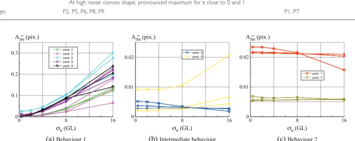
Systematic errors
Let us now focus on the amplitude of the systematic error A—Δu, given in Figure 4 as a function of the standard deviation of the image noise nfor three subset sizes (d = 8, 16 and 32 pixels) and for the intermediate speckle size (r = r0). Results are split into three plots illustrating the observed behaviours as follows: Figure 4A corresponds to behaviour 1 with a strong nonlinear increase of the amplitude with noise level; Figure 4C illustrates behaviour 2 with almost no dependence with noise level. Figure 4B provides results relative to the packages exhibiting some intermediate behaviour. It can be noticed that this error amplitude in general does not depend on the subset size, with the exception of package P4 and, to a limited extent, of package P1, as well as all packages following behaviour 1 at high noise levels. Most packages exhibit a bias amplitude below 0.01 pixel at low noise levels, the maximal amplitude being 0.025 pixel (package P1). At larger noise levels (typically 4 GL on the 256 available levels), the
systematic error can be much larger and becomes a serious limitation of packages following behaviour 1.
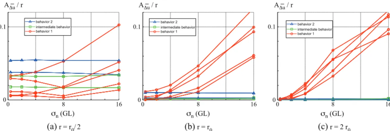
As systematic errors are induced by interpolation procedures aiming at restoring continuous GL (or correlation coefficients) from discrete pixel values, it does make sense to explore the influence of image resolution with respect to speckle size. With this purpose, we compare results obtained with several subsets with the same ratio d/r but different pixel samplings. Three situations are considered as follows: low (r = r0/2 with d = 8 pixels), standard (r = r0and d = 16 pixels) and fine (d = 32 pixels with r = 2r0) spatial image discretisations. This comparison corresponds to the practical situation of the imaging of the same region of interest of a same sample with three different cameras with increasing image definitions (i.e. number of pixels in the image).
In order to compare results in terms of speckle size, systematic error amplitudes are normalised by the speckle size. Results are reported in the three plots in Figure 5, which gives the systematic error amplitude expressed in speckle size as a function of image noise for the three image discretisations. Note that the x and y scales of these plots are the same. The two opposite behaviours in terms of the dependence of the bias amplitude with respect to image noise are again clearly observed on these plots. Packages
Table 2:Summary of observed behaviours. Note that packages P3 and P4 exhibit some intermediate behaviour
Behaviour 1 Behaviour 2 Systematic error Strong dependence of amplitude with noise Almost no dependence with noise Random error -Dependence on n -Less pronounced dependence on n
Very small error at low noise Small error at low noise Similar (average) error at high noise
-Strong dependence on τ -Weak dependence on τ At low noise: concave shape, minimum for τ close to 0 and 1 (Whatever the noise level) At high noise: convex shape, pronounced maximum for τ close to 0 and 1
Packages P2, P5, P6, P8, P9 P1, P7
(a)
Behaviour 1 0 8 16 0 0.1 0.2 0.3 n (GL) Au (pix.) pack. 2 pack. 5 pack. 6 pack. 8 pack. 9 0 8 16 0 0.01 0.02 pack. 3 pack. 4 n (GL) Au (pix.)(b)
Intermediate behaviour 0 8 16 0 0.01 0.02 pack. 1 pack. 7 n (GL) Au (pix.)(c)
Behaviour 2Figure 4: Systematic error amplitude A—Δ
uas a function of noise level nfor three subset sizes (square: d = 8 pixels, triangle: d = 16 pixels, diamond: d = 32 pixels) and standard speckle size (r = r0); behaviour 1 (a), intermediate behaviour (b) and behaviour 2 (c)
following behaviour 1 exhibit in general a lower bias amplitude at low noise, but this tendency is rapidly reversed when image noise increases. In addition, it is observed that for images with low image noise, or for packages following behaviour 2 at any noise level, the bias amplitude can be significantly reduced by increasing the image definition. This reduction is even faster than the decrease in pixel size, which means that a better pixel discretisation leads to a reduced systematic error expressed in pixels (and not only in speckle size). However, for images with high noise levels and for DIC softwares that follow behaviour 1, this reduction of bias amplitude is no longer observed because of the strong influence of image noise for such packages. In such a situation, an increase in image definition, does, in the best case, not lead to any improvement on bias amplitude expressed in speckle size (which means that there is no need in using a higher definition camera) or may even induce an increase of this amplitude. For such packages, there should thus exist some optimal pixel size with respect to speckle size, which would allow us to minimise the bias amplitude. Another implication of these observations is that it does make sense to pre-filter noisy images before processing
them with a package that follows behaviour 1, by means of an N × N binning procedure, which at the same time leads to a reduction of the speckle size with respect to pixel size by a factor N and a reduction of the noise level (assumed independent between adjacent pixels) by the same ratio. An alternative option would be a low-pass pre-filtering (e.g. Gaussian filtering) of the images, which preserve the image definition but reduces both the spatial resolution and the image noise. A thorough examination of the results obtained with commercial codes indeed suggests that some of them, following intermediate behaviour, probably implement such kind of filtering.
Random errors
It has been shown in the Errors versus imposed displacement section that several different behaviours are observed in terms of dependence of random error with imposed displacement τ and noise level (Figure 3). Consequently, random error is now analysed as function of noise level. More particularly, Figures 6, 7 and 8, respectively, present the evolution of the mean random error uover all values of τ for different speckle
0 8 16 0 0.1 behavior 2 behavior 1 intermediate behavior n (GL) A u / r
(a)
r = r0/ 2 0 8 16 0 0.1 n (GL) Au / r behavior 2 behavior 1 intermediate behavior(b)
r = r0 0 8 16 0 0.1 n (GL) Au / r behavior 2 behavior 1 intermediate behavior(c)
r = 2 r0Figure 5: Systematic error amplitude A—Δunormalised by the speckle size as a function of noise level nfor three speckle sizes: (a) r = r0/2, (b)
r = r0, and (c) r = 2r0; subset size proportional to speckle size (i.e. constant d/r, with d = 16 pixels for r = r0)
0 8 16 0 0.05 0.1 u (pix) r = r /2 r = r r = 2r r = r /2 r = r r = 2r n (GL) pack. 2 pack. 5 pack. 6 pack. 8 pack. 9
(a)
Behaviour 1 0 8 16 0 0.05 0.1 u (pix) n (GL) pack. 3 pack. 4(b)
Intermediate behaviour 0 8 16 0 0.05 0.1 u (pix) n (GL) pack. 1 pack. 7(c)
Behaviour 2 r = r /2 r = r r = 2rFigure 6: Mean random error uas a function of noise level for three speckle sizes (square: r = r0/2, triangle: r = r0and diamond: r = 2r0); subset
sizes, the mean random error umultiplied by the subset size d for different subset sizes and the standard deviation uof u,
which quantifies the dependence of this error with τ. To facilitate the interpretation, curves are again presented by distinguishing behaviour 1 (Figures 6A, 7A and 8A), behaviour 2 (Figures 6C, 7C and 8C) and intermediate behaviour (Figures 6B, 7B and 8B), as done in the systematic error analysis presented in the Systematic errors section. It is recalled that the last behaviour corresponds to a behaviour, which generally is intermediate between behaviours 1 and 2 in terms of random error evolution.
For all the packages, the higher the noise level, the higher the mean random error (Figure 6). For low noise levels, u is globally smaller for behaviour 1 than for behaviour 2, particularly for small speckle size (r0/2). For packages related to behaviour 1, u is weakly dependent on speckle size whatever the noise level (and particularly for low noise levels), whereas for packages related to behaviour 2, the quantity u exhibits a more pronounced dependence with speckle size, particularly for low noise levels. For behaviour 2, the smaller the speckle size, the higher the mean random error.
In order to analyse the random error dependency on subset size d, Figure 7 presents the mean random error u multiplied by the subset size d for the standard speckle size r0. This normalisation has been chosen because, at least to first order, random error is essentially inversely proportional to window size. For all the packages, the higher the noise level, the higher the value of (d u), that is to say u decreases with increasing the subset size and increases with the noise level.
For packages following behaviour 1, master curves are obtained with respect to the subset size: for a given package, the evolution corresponding to the three subset sizes are superimposed whatever d (Figure 7A), which confirms, for such procedures, the above mentioned proportionality of u and 1/d. For packages following behaviour 2, higher values of ( d u) are observed for smaller subset sizes than for larger ones, whatever the noise level. Finally, for packages following the intermediate behaviour, no master curve can be extracted either in the evolution of ( d u), although the dependence on the image discretisation seems to be less pronounced than for behaviour 2.
0 8 16 0 8 16 0 8 16 0 1 d = 8 d = 16 d = 32 n (GL) n (GL) n (GL) pack. 2 pack. 5 pack. 6 pack. 8 pack. 9
d u (pix2) d u (pix2) d u (pix2)
(a)
Behaviour 1 0 1 d = 8 d = 16 d = 32 pack. 3 pack. 4(b)
Intermediate behaviour 0 1 d = 8 d = 16 d = 32 pack. 1 pack. 7(c)
Behaviour 2Figure 7: Mean random error multiplied by the subset size (d u) as a function of noise level nfor three subset sizes (square: d = 8 pixels, triangle:
d = 16 pixels and diamond: d = 32 pixels); standard speckle size (r = r0); behaviour 1 (a), intermediate behaviour (b) and behaviour 2 (c)
0 8 16 0 8 16 0 8 16 0 0.025 0.05 0 0.025 0.05 0 0.025 0.05 d = 16 n (GL)
u (pix) u (pix) u (pix)
pack. 2 pack. 5 pack. 6 pack. 8 pack. 9
(a)
Behaviour 1 d = 16 n (GL) pack. 3 pack. 4(b)
Intermediate behaviour d = 16 n (GL) pack. 1 pack. 7(c)
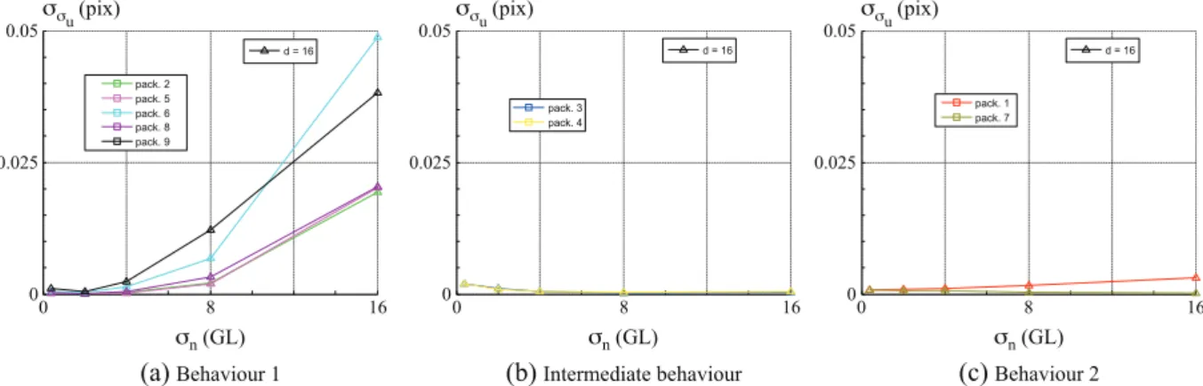
Behaviour 2Figure 8: Standard deviation of the random error uas a function of noise level nfor the standard speckle size r0with d = 16 pixels; behaviour
1 (a), intermediate behaviour (b) and behaviour 2 (c)
The last analysis focuses on the dependence of the random error with the imposed displacement τ. Figure 8 presents the evolution of the standard deviation of the random error u
versus noise level for the case corresponding to subset size d = 16 pixels and standard speckle size r0. Figure 8A corresponding to behaviour 1 clearly shows the strong dependence of the random error with the imposed displacement τ particularly for noisy images. The higher the noise level, the higher the standard deviation of the random error. This trend is a consequence of the evolution of the shape of the random error curve presented in Figure 3 showing that for high noise levels, the random error is very large for τ close to 0 and 1. On the contrary, u is almost independent of the noise level for packages corresponding to behaviour 2 or intermediate behaviour, and values of are at least one order of magnitude below those of packages corresponding to behaviour 1.
Comments and Conclusion
As recalled in the introduction, random and systematic errors observed in the context of the measurement of 2D displacement fields by means of DIC techniques have been addressed by various authors and several strategies. The presently described investigation is based on the analysis of synthetic images, obtained by a numerical process, which closely mimics the image generation in a real digital camera, for both the reference and deformed images. It presents the advantage to be insensitive to image interpolation algorithms which might be used by other methodology to translate images. The error is also quantified exactly because the exact image shift prescribed by the numerical image generation is known, unlike other procedures making use of experimentally recorded images, for which this knowledge depends on the accuracy of the experimental system with which the motion is prescribed or measured. In addition, in our procedure, the dependency of the errors with various image parameters can be investigated separately. Dependence of errors with image noise ( n), speckle size in pixels (r), correlation window size (d) and ratio of correlation windows size to speckle size (d/r) have been established. The most noticeable novelty of the presented benchmark is related to the unprecedented wide range of DIC formulations and packages that have been tested and compared on the same set of images.
This last aspect allows to clearly establish some generic behaviours common to all packages, such as the existence of an S-shaped systematic error curve, the increase of random errors with image noise and its decrease with window size (in the present context of the absence of shape function mismatch error). More importantly, it allowed us to establish clear differences in the behaviour of different algorithms or implementations. The precise shape and amplitude of the systematic error curve are, for instance,
very different from one package to the other. It is however possible to gather most DIC packages into two families exhibiting similar behaviours in terms of evolution of systematic and random errors with respect to image noise n and subpixel displacement τ, as summarised from a qualitative point of view in Table 2. This separation into two families has again been observed and analysed more quantitatively in the Systematic errors and Random errors sections. Family 1, for instance, exhibits an almost ideal proportionality of average random errors with d and an almost linear dependence of random error with n, while such rules do not apply for packages of family 2. On the other hand, random errors are almost insensitive to subpixel displacement for family 2, while a complex dependence, which strongly evolves with nis observed for family 1. In terms of systematic errors, the strong increase with noise of the amplitude of the S-shaped curve for family 1 has been quantitatively confirmed for all packages of this family, with similar but not identical amplitudes of these errors. The quasi-independence of the systematic error amplitude with n for packages of family 2 is confirmed over the whole range of investigated image noise and various image definitions (i.e. speckle size expressed in pixels, at fixed d/r). The strong influence of this last parameter on systematic errors has also been confirmed in our study: a better image definition allows reducing systematic errors but only under the condition that image noise remains sufficiently low in the case of family 1. Generally speaking, packages of the first family lead to lower error levels (both random and systematic) when the imaging conditions are good (i.e. low image noise and sufficient image definition), but packages of family 2 are much more robust to image noise.
Roughly speaking, the packages associated with the first family globally lead to better results when the noise standard deviation is smaller than 4 GL because of the low levels of random errors they generate in that context. Packages of family 2 behave more efficiently for noise levels above 8 GL, essentially not only because of their noticeably reduced amplitude of systematic errors but also because of their slightly reduced random error. This behaviour of the packages of family 2 might be explained, at least qualitatively, by their implementation, based on subpixel optimisation making use of an interpolation of the correlation coefficient, instead of GL interpolation used in packages of family 1. This seems to provide the DIC packages of family 2 some noise-filtering capacity to the detriment of larger random errors in the case of small subsets and no image noise, even though no explicit pre-filtering of the images is performed by these packages, at least for one of them. Indeed, for images with low noise, the interpolation of the correlation coefficient from values at discrete translations by an a priori (usually quadratic) function is likely to be less accurate than the computation of the correlation coefficient for any subpixel translation.
Consequently, a higher error (likely to be essentially random) might be expected on the optimal value of this translation.
A practical implication of these observations for a DIC user is the following. If the images are of good quality, i.e. exhibit low noise level, algorithms of family 1 will provide better results; but in case of high noise level, two options are possible: either use family 2 algorithms or apply family 1 algorithms on pre-filtered images. Another practical implication of our observations is that there is no need to increase the resolution of the images with respect to the speckle size in case of highly noisy images as commented in the Systematic errors section. At this stage, it is however difficult to provide more specific recommendations, for instance, in terms of choice of GL interpolation or correlation coefficient for packages following behaviour 1, as no definitive trends can be emphasised as commented above. Our results show on the contrary that one should be cautious when using DIC algorithms, when accuracy is a concern. Some trends observed in some cases might indeed not apply to other situations, so that no direct solution can be suggested. Parameter sets providing low errors, either systematic or random, in some cases might be much less efficient in others and conversely. Error analysis requires thus to be performed for each situation, which somewhat limits the versatility of DIC systems for non-specialised users and suggests the necessity to develop tools to quantify errors adapted to real situations, such as the one presented here.
Some of the observed behaviours, especially those exhibited by family 1, have already been reported in the literature [13, 33], and analytical models have recently been provided for them. In particular, the perturbation analysis proposed by [13], when specialised to pure translation, predicts a linear dependence of random errors with image noise (when white noise is assumed as in this study). In addition, for a stationary speckle pattern and sufficiently large window sizes, these errors evolve like 1/d, as almost observed in our results, in the case of family 1. Such an analysis has been extended by [33] to take into account the discrete nature of images and the influence of GL interpolation; the dependence of systematic error with noise could for instance be predicted.
A quantitative comparison with these analytical models could be proposed. However, such a comparison will require additional developments and will be the object of a forthcoming paper. As can for instance be seen in Figures 4A, 6A and 7A, the coefficients governing the dependence of random errors with image noise and window size depend on the packages, even though they are similar. The dependence of these coefficients with the particular options used by the packages (such as type of correlation coefficient and GL interpolation routine) needs thus to be taken into account. A similar comment holds if amplitude of systematic
errors would have to be compared to the model proposed in [33], which has been developed for a specific correlation coefficient and for bilinear and bicubic GL interpolation. It can also be noticed that the strong dependence of random errors with subpixel translation, especially for high noise level, as observed here and in earlier studies [34], is not predicted by any of these models and will require additional modelling efforts.
Let us also notice that even if the presented results are specific to a particular modelled speckle pattern, the procedure could be extended to any other one, including experimental ones, if an appropriate theoretical model is available or if a way to record them at sufficiently high resolution is available, in the line of [22]. Some generic information on the behaviour of some DIC packages with respect to some image properties or DIC parameters have also been evidenced in our study and suggest possible ways to improve DIC performances. In particular, the evolution of systematic errors with image definition and image noise evidenced at the end of Systematic errors section suggests that there is a way to optimise image acquisition conditions with respect to these errors. For a given noise level (linked to the camera) and physical size of the speckle pattern (provided for instance by the natural structure of the sample), there must exist an optimal optical magnification, which minimises systematic errors, at least for family 1. Moreover, some pre-processing of the images (such as pixel binning as suggested at the end of Systematic errors section), leading to a reduced noise level and smoother images might also improve results and might be tested for a given experimental setup.
ACKNOWLEDGEMENTS
The authors gratefully acknowledge the French CNRS (National Centre for Scientific Research) for supporting this research through the GDR2519 research network ‘Mesures de Champs et Identification en Mécanique des Solides’. REFERENCES
1. Sutton, M. A., Orteu, J.-J. and Schreier, H. W. (2009) Image Correlation for Shape, Motion and Deformation Measurements -Basic Concepts, Theory and Applications. Springer.
2. Pan, B., Qian, K., Xie, H. and Asundi, A. (2009) Two-dimensional digital image correlation for in-plane displacement and strain measurement: a review. Meas. Sci. Technol. 20, 062001
3. Rastogi, P. K. (2000) Photomechanics, Topics in Applied Physics Series, Vol. 77. Springer-Verlag, Berlin Heidelberg New York.
4. Grédiac, M. and Hild, F. (Eds) (2012) Full-Field Measurements and Identification in Solid Mechanics. ISTE Ltd and John Wiley & Sons Inc.
5. Bornert, M., Brémand, F., Doumalin, P., et al. (2009) Assessment of digital image correlation measurement errors: methodology and results. Exp. Mech. 49, 353–370.
6. Bornert, M. (2006) Resolution and spatial resolution of digital image correlation techniques. In: Photomechanics 2006. Clermont-Ferrand, France.
7. Dupré, J. C., Bornert, M., Robert, L. and Wattrisse, B. (2010) Digital image correlation: displacement accuracy estimation. Proc. International Conference on Experimental Mechanics (ICEM’14), Poitiers, France.
8. Chu, T. C., Ranson, W. F., Sutton, M. A. and Peters, W. H. (1985) Applications of digital image-correlation techniques to experimental mechanics. Exp. Mech. 25, 232–244.
9. Sutton, M. A., McNeill, S. R., Jang, J. and Babai, M. (1988) Effects of subpixel image restoration on digital correlation error estimates. Opt. Eng. 27, 870–877.
10. Choi, S. and Shah, S. P. (1997) Measurement of deformations on concrete subjected to compression using image correlation. Exp. Mech. 37, 307–313.
11. Wang, Y. and Cuitino, A. M. (2002) Full-field measurements of heterogeneous deformation patterns on polymeric foams using digital image correlation. Int. J. Solids Struct. 39, 3777–3796. 12. Dautriat, J., Bornert, M., Gland, N., Dimanov, A. and Raphanel,
J. (2011) Localized deformation induced by heterogeneities in porous carbonate analysed by multi-scale digital image correlation. Tectonophysics 503, 100–116.
13. Roux, S. and Hild, F. (2006) Stress intensity factor measurements from digital image correlation: post-processing and integrated approaches. Int. J. Fract. 140, 141–157.
14. Triconnet, K., Derrien, K., Hild, F. and Baptiste, D. (2009) Parameter choice for optimized digital image correlation. Opt. Lasers Eng. 47, 728–737.
15. Hua, T., Xie, H., Wang, S., Hu, Z., Chen, P. and Zhang, Q. (2011) Evaluation of the quality of a speckle pattern in the digital image correlation method by mean subset fluctuation. Opt. Laser Technol. 43, 9–13.
16. Pan, B., Lu, Z. and Xie, H. (2010) Mean intensity gradient: an effective global parameter for quality assessment of the speckle patterns used in digital image correlation. Opt. Lasers Eng. 48, 469–477.
17. Wattrisse, B., Chrysochoos, A., Muracciole, J.-M. and Némoz-Gaillard, M. (2000) Analysis of strain localization during tensile tests by digital image correlation. Exp. Mech. 41, 29–39. 18. Lecompte, D., Smits, A., Bossuyt, S., Sol, H., Vantomme,
J., Van Hemelrijck, D. and Habraken, A. M. (2006) Quality assessment of speckle patterns for digital image correlation. Opt. Lasers Eng. 44, 1132–1145.
19. Lava, P., Cooreman, S., Coppieters, S., De Strycker, M. and Debruyne, D. (2009) Assessment of measuring errors in DIC using deformation fields generated by plastic FEA. Opt. Lasers Eng. 47, 747–753.
20. Koljonen, J. and Alander, J. T. (2008) Deformation image generation for testing a strain measurement algorithm. Opt. Eng. 47, 107202.
21. Bornert, M., Doumalin, P., Dupré, J.-C., Poilâne, C., Robert, L., Toussaint, E. and Wattrisse, B. (2012) Short remarks about synthetic image generation in the context of the assessment of sub-pixel accuracy of Digital Image Correlation. Proc. International Conference on Experimental Mechanics (ICEM’15), Porto, Portugal.
22. Reu, P. (2011) Experimental and numerical methods for exact subpixel shifting. Exp. Mech. 51, 443–452.
23. Schreier, H. W., Braasch, J. R. and Sutton, M. A. (2000) Systematic errors in digital image correlation caused by intensity interpolation. Opt. Eng. 39, 2915–2921.
24. Zhoun, P. and Goodson, K. E. (2001) Subpixel displacement and deformation gradient measurement using digital image/ speckle correlation (DISC). Opt. Eng. 40, 1613.
25. Pan, B., Xie, H.-M., Xu, B. Q. and Dai, F. L. (2006) Performance of sub-pixel registration algorithms in digital image correlation. Meas. Sci. Technol. 17, 1615–1621.
26. Sousa, A. M. R., Xavier, J., Vaz, M., Morais, J. J. L. and Filipe, V. M. J. (2011) Cross-correlation and differential technique combination to determine displacement fields. Strain 47, 87–98.
27. Zhang, J., Cai, Y., Ye, W. and Yu, T. X. (2011) On the use of the digital image correlation method for heterogeneous deformation measurement of porous solids. Opt. Lasers Eng. 49, 200–209. 28. Orteu, J.-J., Garcia, D., Robert, L. and Bugarin, F. (2006) A
speckle texture image generator. Proc. SPIE 6341, Speckle06: Speckles, From Grains to Flowers, Nîmes, France (September 15, 2006); doi: 10.1117/12.695280.
29. Doumalin, P., Bornert, M. and Caldemaison, D. (1999) Microextensometry by image correlation applied to micromechanical studies using the scanning electron microscopy. Proc. International conference on advanced technology in experimental mechanics, Ube City, Japan, 81–86.
30. Schreier, H. W. and Sutton, M. A. (2002) Systematic errors in digital image correlation due to undermatched subset shape function. Exp. Mech. 42, 303–310.
31. Oriat, L. and Lantz, E. (1998) Subpixel detection of the center of an object using a spectral phase algorithm on the image. Pattern Recognit. 31, 761–771.
32. Poilâne, C., Lantz, E., Tribillon, G. and Delobelle, P. (2000) Measurement of in-plane displacement fields by a spectral phase algorithm applied to numerical speckle photography for microtensile test. Eur. Phys. J. Appl. Phys. 11, 131–145.
33. Wang, Y. Q., Sutton, M. A., Bruck, H. A. and Schreier, H. W. (2009) Quantitative error assessment in pattern matching: effects of intensity pattern noise, interpolation, strain and image contrast on motion measurements. Strain 45, 160–178. 34. Doumalin, P. (2000) Microextensométrie locale par
corrélation d’images numériques – Application aux études micromécaniques par microscopie électronique à balayage. PhD thesis. Ecole Polytechnique, 260 p. (in French).
APPENDIX A: ESTIMATION OF QUANTISATION NOISE
Let us consider the recording of images obtained by converting photons collected over a time-range large enough to consider the conversion as a time-independent process. The electrical charge of a given pixel, denoted x herein, can take NQ= w/2b distinct values inside a quantisation interval (providing the same digital value), where w is the electronic well depth and b is the number of considered bits. NQis sensor dependent and is usually at least NQ= 100, so that x is considered to be continuous in the following. Furthermore, we assume that the charge x is corrupted by thermal fluctuations as well as fluctuations of
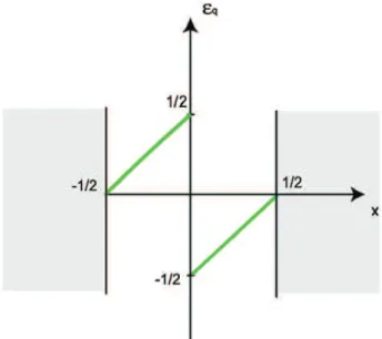
the number of photons impinging on the considered pixel (shot-noise). Let us assume these fluctuations are large enough to consider all charge values equally probable over the quantisation interval. The quantisation error εq(x) on the electrical charge is defined as the difference between the actual charge x and its rounded value A(x)
εqð Þ ¼ x # A xx ð Þ
This error is periodic with a one quantisation step period, corresponding to 1 GL, and its variation on the interval [#0.5 NQ, 0.5 NQ], expressed on the GL scale, is illustrated in Figure A1.
The expectation of εq(x) is equal to hεq(x)i, with hXi standing for the integrated value of X over the quantisation interval, because all charge values are assumed equally probable. Using the analytical definition of εq(x), it is immediate to see that this expectation is equal to zero. Consequently, the variance of εq(x) is equal tohεq2(x)i, which can be easily calculated, and is equal to 1/12.
The quantisation contribution to the noise corrupting a digital image is described by the distribution of A(x). Its expectation is equal to
A xð Þ
h i ¼ xh i # εqð Þx! ¼ xh i
The variance of A(x) is obtained as
A2 x ð Þ! ¼ x2! # 2 x ε qð Þx! þ ε2qð Þx D E ¼ x2! þ1 6 using the identity x εqð Þx ! ¼ #241
The noise of the digitised data A(x) can be defined as the standard deviation of A(x), denoted here A
2 A¼ A2ð Þx ! # A xh ð Þi 2 ¼16þ x2! # x h i2¼16þ 2 x where 2 x¼ x2! # xh i 2
denotes here the variance of x. Considering noiseless images ( x= 0), the standard deviation describing the noise of the digitised data reduces to the quantisation noise A, which is shown to be equal to q¼ 1=
ffiffiffi 6 p
≈0:4 GL. For real-life images, the quantisation contribution may turn negligible so that A≈ xsince other sources of noise – depending on both the sensor and the measured photon flux – may dominate. For instance, for x greater than 2 GL, the quantisation contribution represents less than 2% of the x.
Figure A1: Variations of the quantisation error εq(x) as a function of