HAL Id: hal-00365304
https://hal.archives-ouvertes.fr/hal-00365304
Submitted on 2 Mar 2009
HAL is a multi-disciplinary open access
archive for the deposit and dissemination of
sci-entific research documents, whether they are
pub-lished or not. The documents may come from
teaching and research institutions in France or
abroad, or from public or private research centers.
L’archive ouverte pluridisciplinaire HAL, est
destinée au dépôt et à la diffusion de documents
scientifiques de niveau recherche, publiés ou non,
émanant des établissements d’enseignement et de
recherche français ou étrangers, des laboratoires
publics ou privés.
Lucien Wald, Thierry Ranchin, Marc Mangolini
To cite this version:
Lucien Wald, Thierry Ranchin, Marc Mangolini. Fusion of satellite images of different spatial
reso-lutions: Assessing the quality of resulting images. Photogrammetric engineering and remote sensing,
Asprs American Society for Photogrammetry and, 1997, 63 (6), pp.691-699. �hal-00365304�
FUSION OF SATELLITE IMAGES OF DIFFERENT SPATIAL RESOLUTIONS: ASSESSING THE QUALITY OF RESULTING IMAGES
(1) Lucien WALD, (1) Thierry RANCHIN, (2) Marc MANGOLINI
(1) Ecole des Mines de Paris, Groupe Télédétection & Modélisation, BP 207, 06904 Sophia Antipolis cedex, France
(2) Aérospatiale, Service Télédétection, BP 99, 06332 Cannes la Bocca cedex, France
Published in Photogrammetric Engineering & Remote Sensing, vol. 63, no 6, 691-699, June 1997. Has received the 1997 Autometrics Award.
ABSTRACT
Methods have been proposed to produce multispectral images with enhanced spatial resolution using one or more images of the same scene of better spatial resolution. Assuming that the main concern of the user is the quality of the transformation of the multispectral content when increasing the spatial resolution, this paper defines the properties of such enhanced multispectral images. It then proposes both a formal approach and some criteria to provide a quantitative assessment of the spectral quality of these products. Five sets of criteria are defined. They measure the performance of a method to synthesize the radiometry in a single spectral band as well as the multispectral information when increasing the spatial resolution. The influence of the type of landscape present in the scene upon the assessment of the quality is underlined, as well as its dependence with scale. The whole approach is illustrated by the case of a SPOT image and three different standard methods to enhance the spatial resolution.
Keywords: fusion, image quality, multisensor, multiresolution.
Running title: Fusion of satellite images of different spatial resolutions.
INTRODUCTION
Many works have recognized the benefit of merging high spectral resolution (or spectral diversity) and high spatial resolution images, particularly in land mapping applications. Some satellite systems offer both kinds of data. The Landsat Thematic Mapper (TM) system presents six spectral visible and near-infrared bands with a 30 m resolution and a thermal near-infrared band with a 120 m resolution. The present SPOT system has three spectral bands with a 20 m resolution (called XS1, XS2, XS3) together with a
panchromatic band of 10 m resolution (called P). The next SPOT systems will have more spectral bands and enhanced spatial resolutions, and will also retain this dual resolution capability. Besides these widely used systems, other systems offer either spectral capabilities or high spatial resolution, including the Russian KFA and KVR systems, with resolutions of 10 to 2 m, and other systems to come from United States and elsewhere. This list does not pretend to be exhaustive and is intentionally restricted to the systems presently used for fine-scale land mapping. It illustrates the diversity of available data which can be merged together for a better knowledge of our environment.
Many methods have been proposed for the merging of high spectral and high spatial resolution data in order to produce multispectral images having the highest spatial resolution available within the data set. We are only concerned with those methods which claim to provide a synthetic image close to reality when enhancing the spatial resolution, and not those which only provide a better visual representation of the image (e.g., Carper et al., 1990). Some methods are specific to the case of SPOT (Anonymous, 1986; Pradines, 1986), while others are more general (Blanc et al., 1996; Chavez et al., 1991; Garguet-Duport
et al., 1994; Garguet-Duport et al., 1996; Li et al., 1995; Iverson and Lersch, 1994; Mangolini et al.,
1992; Mangolini et al., 1993; Munechika et al., 1993; Pellemans et al., 1993; Tom, 1987; Yocki, 1996). These methods make use of the data having the best spatial resolution to simulate multispectral images at this resolution. However no methods propose any assessment of the quality of the resulting synthetic images except for Blanc et al., Mangolini et al., Munechika et al. and Li et al., the last approach being rather inapplicable to Earth images.
The goal of the present paper is to propose both an approach and some criteria for a quantitative assessment of the quality. In doing this, we assume that the main demand of the user concerns the quality of the transformation of the multispectral content when increasing the spatial resolution. The better the simulation of the spectral content at the enhanced resolution, the more accurate the classification for mapping purposes. Our approach is similar in essence to the one used by Mangolini et al. (1992) and, for the case of SPOT, by Mangolini et al. (1993, 1995) and Munechika et al. (1993). The present work offers a more extensive discussion of the approach and proposes a formalism as well as quality criteria. The influence of the resolution itself with respect to the type of landscape upon the assessment of the quality is finally discussed.
BACKGROUND
At first some general comments are needed, in particular regarding the superimposability of images and the simultaneity of their acquisition by the sensors. The above-mentioned methods require superimposable images, once all images are set to the lowest available spatial resolution (e.g., 20 m in the
case of SPOT). Some images are already co-registered, such as Landsat images. Otherwise this can be done by means of standard methods available in public or commercial software packages for image processing. The images of lowest resolution (e.g., XS in the case of SPOT) are projected into the geometry of the image of highest resolution (e.g., P in the SPOT case) degraded to the lowest resolution (e.g., 20 m in the SPOT case). During the process, a resampling of the multispectral images is made. The resampling operator has an influence upon the final result. In most cases, a bi-cubic interpolator offers a good compromise between the accuracy of the result and the required computer time. In the following, for the sake of the simplicity, the term "image of lowest resolution" will denote the projected resampled image of lowest resolution, if this is required.
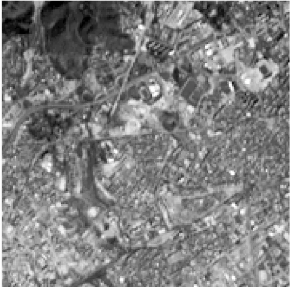
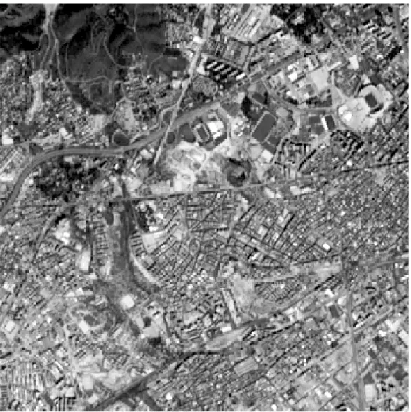
The images of different resolutions may not have been acquired simultaneously. Optical properties of the atmosphere are different from one date to the other. This induces further spectral distortion in the set of images. As for the landscape, as long as the time-lag is small with respect to the time scale of the variations in small-size features, its influence upon the quality of the transformation of the spectral content when enhancing the spatial resolution is low or negligible. Such a time scale is greatly variable and does depend upon the objects themselves as well upon the spatial and spectral resolutions with which they are observed. If the time-lag is large, the user must weight its consequences. He should know precisely the merging method to be used, because all methods do not take into account in the same way the small structures to be injected from the images of highest resolution into the images of lowest resolutions. For example, Anonymous (1986) recommends that its method should be used only for coincident SPOT XS and P data. This method from the CNES (French space agency) is called P+XS and is certainly the most commonly used method among those cited above. However, it is frequently applied to non-coincident SPOT data because of the difficulties in obtaining coincident couples of images. The quality of the resulting synthetic images is usually assessed by visual inspection, a necessary step. For example, Figures 1 to 4 present a SPOT sub-scene of Barcelona., acquired on 11 September 1990. Barcelona is a large city located in north-east Spain, on the Mediterranean coast. Its harbor is the busiest in Spain. This extract of the SPOT scene displays the western, newest districts of the city. Displayed is only a part (360 by 360 pixels) of the sub-scene (512 by 512 pixels) which is dealt with in the following sections. The sub-scene is mostly comprised of urban districts, highways and railroads. It also exhibits small agricultural lots and mountainous areas covered by typical Mediterranean vegetation. Such an urban area has been selected for illustration because it is certainly the most difficult type of landscape to deal with according to our knowledge. Urban areas often point out the qualities and drawbacks of algorithms because of the high variability of information in space and spectral band, induced by the diversity of features both in size and nature.
The panchromatic band P is shown in Figure 1, while the XS1 is in Figure 2. The latter has been magnified by a factor of two. In Figure 3 is the synthetic image obtained by the CNES method (XP1), and in Figure 4, the synthetic one obtained by the ARSIS method (XS1-HR). These methods are discussed later. When comparing images, one must pay attention to the contrast table (look-up table) because it acts as a filter (together possibly with the printer) between the information and the human observer. In the case of SPOT, the radiances observed in the P, XS1, and XS2 bands are very similar for a spectrally neutral target. For a spectral band i, the radiance Ri is linked to the digital count DCi by the calibration factor ai: i.e.,
Ri = DCi / ai
In this particular case, the calibration factors are very similar for the P and XS1 bands (see Table 1), and, thus, so are the digital counts. It follows that the same look-up table can be applied to each image in Figures 1 to 4 and that they can be visually compared. Beyond demonstrating the interest of merging P and XS data, visual inspection clearly shows the major drawbacks of both methods. In Figure 3, local contrasts are too much reinforced. The extreme values are also reinforced: the white areas are whiter, compared to Figure 2, and the dark areas are darker. In Figure 4, on the contrary, one may think that local contrasts are too smooth, but gray tones are very similar to Figure 2.
The objective comparison of the visual quality of multiple images is a difficult and lengthy task to handle. The human visual system is not equally sensitive to various types of distortion in an image. The perceived image quality is strongly dependent upon the observer and also upon the thematic application. Standard protocols have been defined, namely in the field of television and image compression. Such a protocol is described, for example, in Lu et al. (1996) for the compression of still images. A panel of human viewers judge some well-defined aspects of the images. Then their notations are weighted and further processed to obtain a mean opinion score defining the quality of the result. When it comes to the assessment of the quality of a set of multispectral images, the mass of data becomes very large. This dramatically increases the difficulty in computing a quantitative picture quality scale. Beyond the visual inspection, mathematical criteria are needed.
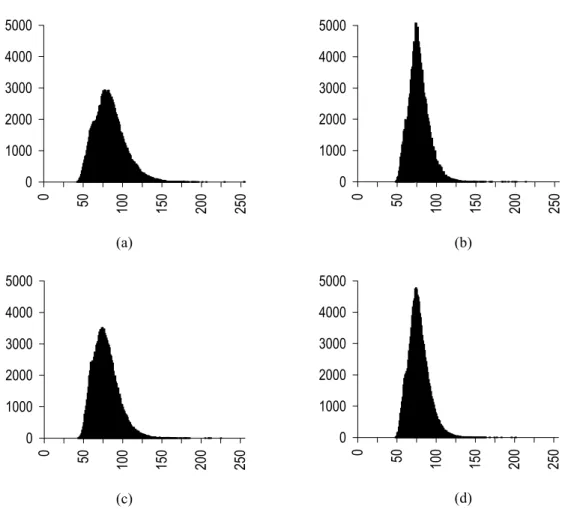
One simple way is to look at the histograms of the synthetic products and to compare them to the original ones. The histograms for the previous images (Figures 1 to 4) are presented in Figure 5. On the upper half are those for the original images P and XS1. For the latter, the resolution is 20 m only: it contains four times fewer pixels than P or the synthetic images. For the comparison, the XS1 histogram has been normalized to the others by multiplying the number of pixels by four. Though the resolution is increased by a factor of two relative to XS1, the histograms of the synthetic images are expected to be close to the
XS1 one in shape. This is true for the XS1-HR histogram. Its highest frequency is close to four times the peak of XS1. On the contrary, the XP1 histogram is much closer to the P one, both in shape and in peak. This comparison of histograms is a fairly good estimator of image quality, and is easy to handle. However, the effect of the spatial resolution upon the statistical properties of an image should not be neglected (e.g., Kong and Vidal-Madjar, 1988; Woodcock and Strahler, 1987; Raffy, 1993; Welch et al., 1989). That means that we should not try to identify the statistical properties of a synthetic product to those of the original image. These discrepancies in statistics depend upon the observed type of landscape. Therefore, other mathematically-sound criteria are needed.
Another approach is to compare land-use maps obtained after spectral (and possibly textural) classification of the synthetic images. These maps are compared either to the map obtained from original low-resolution data (e.g., SPOT XS), or to ground truth. In the first case, the same assumption as above is made, that some statistical properties are preserved through the increase in resolution. Hence, this approach should be avoided. More generally, classification greatly reduces the content in information, making discrepancies between methods disappear. For example, Munechika et al. (1993) compared their method to Price's one (1987) for Landsat-TM. On the one hand they obtained a large relative difference between both methods - which we have estimated at about 25 % (RMS) according to the figures available in their paper - while, on the other hand, the classification rates were very similar. This classification approach is valuable because land-use mapping is often the goal of satellite image processing. However, it may not reflect the overall performance of a method since the results depend too much upon the type of landscape, its diversity, its heterogeneity, the time of observation, the optical properties of the atmosphere, the sensor system itself (including the viewing geometry), the type of classifier (supervised, unsupervised), and the classifier itself.
The type of landscape present within the image used to assess the quality of a synthesizing method has a strong influence upon the results. Whatever the method, the more predictable the change in signal with the scale, the better the quality of the final product. Over areas such as the ocean or large agricultural lots, which appear very homogeneous at, say, 20 m resolution, the error made in assuming that these areas are still homogeneous at, say, 10 m resolution, is small. On the other hand, urban areas or small agricultural lots are among the most difficult cases because they exhibit a large number of interwoven objects having different scales. Wald and Ranchin (1995) examined the SPOT image of Barcelona presented above. They found that, for the homogeneous part covering the Mediterranean Sea (not visible in Figures 1 to 4, and actually not within the sub-scene used for illustration), all information, expressed as variance, is borne by structures larger than 40 m. On the contrary, for the urban area, half the information is borne by structures having sizes less than 40 m. Such cases do not possess self-similarity properties, though some parameters, such as the growth of city limits, can be approximated by fractal functions (e.g., Batty, 1991).
In other words, structures observed at, say, 10 m resolution, cannot be accurately predicted from their observations at lower resolution, say, 20 m. This is well-known by experienced image interpreters, and is also sustained by mathematical evidence (e.g., Fung and Chan, 1994; Ramstein, 1989; Woodcock and Strahler, 1987). The benefit of an image of a higher spatial resolution is the greatest in these cases. Hence, we recommend that test images should mainly include such areas. Such cases also offer a large diversity of spectral signatures, which is helpful in judging the ability of a method to synthesize the spectral signatures during the change in spatial resolution.
A FORMAL APPROACH FOR QUALITY ASSESSMENT OF THE RESULTING SYNTHETIC IMAGES
Let denote the images of lowest resolution by Ml, and the images of highest resolution by Ph. The
subscripts l and h denote the resolution of image M or P, i.e., low and high resolution, respectively. The subscript s (for small) is to be used later: it denotes a resolution which is lower than l, say, e.g. two times
lower. According to the previous section, the images Ml and Pl are superimposable. Both Ml and Ph have
been obtained by a sensor. The merging method aims at constructing synthetic images M*h.
These synthetic images must have the three following properties. First, any synthetic image M*h, once
degraded to its original resolution l, should be as identical as possible to the original image Ml. For
example, in the case of SPOT, the synthetic image is called XS*10. Once resampled to 20 m, this image
should be as close as possible to the original XS image. Besides the effects induced by time-lag in image acquisition, as discussed in previous section, observing this property means that the method takes into account the differences in atmospheric effects affecting the images of lowest and highest resolutions
which have not been acquired within the same spectral bands. Second, any synthetic image M*h should be
as identical as possible to the image Mh that the corresponding sensor would observe with the highest
resolution h. Because the synthetic image M*h do not match Mh exactly, a property should be added,
dealing with the entire set of channels. Third, the multispectral set of synthetic images M*h should be as
identical as possible to the multispectral set of images Mh that the corresponding sensor would observe
with the highest resolution h. In the case of SPOT, this set of synthetic images is the triplet (XS1*10,
XS2*10, XS3*10). The assessment of the quality of the resulting spatially enhanced spectral images is now
equivalent to the verification of these properties.
Testing the first property: Any synthetic image M*h, once degraded to its original resolution l, should be
as identical as possible to the original image Ml. To achieve this, the synthetic image M*h is spatially
degraded to an approximate solution M’l of Ml. If the first property is true, then M’l is very close to Ml.
visually compared to the original image in order to detect trends of error, if any, possibly related to the type of landscape. Then some statistical quantities are to be used to quantitatively express the discrepancies between both images. These quantities are similar to the first and second sets of criteria described under the second property below.
An important point here is the way the synthetic image M*h is degraded to M’l. Some wavelet transforms
have the ability to separate scales well, that is, to separate small size structures from larger ones and, therefore, to fairly well simulate what would be observed by a lower resolution sensor (e.g., Ranchin and Wald, 1993). Munechika et al. (1993) used an averaging operator on a window of 3 by 3 pixels. Such an operator does not have this ability and is not as appropriate here. Other filtering operators can be used, some of them simulating a given modulation transfer function (MTF) of a sensor. A comparison was made on a few scenes using some operators, such as the truncated Shannon function, bi-cubic spline, pyramid-shaped weighted average, and wavelet transforms of Daubechies (1988, regularity of 2, 10 and 20). It showed relative discrepancies between the results on the order of a very few per cent. In conclusion, there is an influence of the filtering operator upon the results, but it can be kept very small provided the operator is appropriate enough.
Testing the second property: Any synthetic image M*h should be as identical as possible to the image Mh
that the corresponding sensor would observe with the highest resolution h. The second and third
properties are difficult to test, because they refer to Mh, an image that would be sensed if the sensor had a
better resolution. This image, of course, is not available; otherwise, all the above-cited methods would not have been developed. The difficulty is partly overcome by the following approach:
- The available images Ph and Ml are degraded to respectively Pl and Ms, respectively. For the SPOT
case, the P and XS images are degraded to P20 (20 m resolution) and XS40 (40 m resolution). The
images Pl and Ms are very close to what the corresponding sensor would have measured with a
degraded resolution, as discussed previously.
- Then the synthesizing method under assessment is applied to Pl and Ms. It provides a synthetic image
M*l (XS*20 in the SPOT case).
- This synthetic image M*l is compared to the image-truth Ml (XS in the SPOT case) by means of some
criteria described below. The numerical comparison should be made preferably in physical units and also in relative values. Thus, different tests made over different scenes may be compared.
- This comparison provides an assessment of the quality of M*l. It is assumed that this quality is fairly
similar to that of the synthesized high-resolution image M*h. This point will be discussed later.
Such an approach was made by Munechika et al. (1993) and Mangolini et al. (1992, 1995). To assess the
property. After visual inspection, the difference image is reduced to a few statistical parameters which summarize it. There are a large number of candidate parameters. We have computed many for several tens of cases. We have retained some whose definitions are well-known to engineers and researchers and which clearly characterize the advantages and disadvantages of a method.
Two sets of criteria are proposed to quantitatively summarize the performance of a method in synthesizing an image in one spectral band. The first set of criteria provides a global view of the
discrepancies between the original image Ml and the synthetic one M*l. It contains:
- The bias, as well as its value relative to the mean value of the original image. Recall that the bias is the difference between the means of the original image and of the synthetic image. Ideally, the bias should be null.
- The difference in variances (variance of the original image minus variance of the synthetic image), as well as its value relative to the variance of the original image. This difference expresses the quantity of information added or lost during the enhancement of the spatial resolution. For a method providing too many innovations (in the sense of information theory), i.e., "inventing" too much information, the difference will be negative because the variance of the synthetic image will be larger than the original variance. In the opposite case, the difference will be positive. In information theory, the entropy describes the quantity of information. However, we selected the variance difference because most researchers and engineers are much more familiar with variance, and entropy and variance act quite similarly for our purpose. Ideally, the variance difference should be null.
- The correlation coefficient between the original and synthetic images. It shows the similarity in small size structures between the original and synthetic images. It should be as close as possible to 1. - The standard deviation of the difference image, as well as its value relative to the mean of the original
image. It globally indicates the level of error at any pixel. Ideally, it should be null.
The error at pixel level may be more detailed. Let us compute at each pixel the absolute relative error (the absolute value of the difference between the original and synthetic values, divided by the original value). Then the histogram of these relative errors is computed. It can be seen as the probability density function. Therefore, we can compute the probability of having at a pixel a relative error (in absolute value) lower than a given threshold. This probability denotes the error made at pixel level, and hence indicates the capability of a method to synthesize the small size structures. The closer to 100 percent the probability for a given error threshold, the better the synthesis. The ideal value is a probability of 100 percent for a null relative error. Here, for reasons of computer precision, the lowest threshold "no relative error or null error" is set to 0.001 percent
Testing the third property: The multispectral set of synthetic images M*h should be as identical as possible to the multispectral set of images Mh that the corresponding sensor would observe with the highest resolution h. Visual inspection may be made through color composites of, for example, the first
three principal components of the set of images. Both color composites should agree visually. Most methods for color composites are using dynamical adjustment for color coding (e.g., Albuisson, 1993). If the sets of images are different, even slightly, then the color coding will be different for both composites and no comparison will be possible. Practically, we recommend the following approach. For each spectral
band, the Ml and M*l images are juxtaposed into a single computer file. The principal components
analysis as well as the color coding are performed on this set of files. The projected Ml and M*l images
are then extracted from these projected files and the color composites are displayed, simultaneously or alternatively, onto the screen. This approach guarantees that the color composites are comparable. Of course, if only three spectral bands are available as in the SPOT case, there is no need to perform a principal components analysis. The advantage of this visual assessment is that it does show trend in errors, if any, possibly related to landscape features. The drawback of it is that it is a subjective assessment and also that this assessment may be limited either by physiological factors (e.g., color contrast perception by humans), or by technical factors (e.g., when a large number of spectral bands are present). In the latter case, and if the landscape offers a large variety of objects, the color re-coding of the
first three principal components reduces dramatically the differences between the Ml and M*l images,
particularly if these differences are random, i.e., not related to a peculiar landscape feature or to a spectral band.
A quantitative assessment can be made using the following three additional sets of criteria which quantify the performance of a method to synthesize the spectral signatures during the change in spatial resolution. The third set (numbered after the two sets described above for the second property) deals with the information correlation between the different spectral images taken two at a time. This dependence can be expressed by the correlation coefficients, with the ideal values being given by the set of original images
Ml. As an example, for the case of SPOT, the correlation coefficient between P20 and XS1*20 is computed
and compared to the correlation coefficient for P20 and XS120. This is done for every pair. The fourth set
of criteria partly quantifies the synthesis of the actual multispectral n-tuplets by a method, where n-tuplet means the vector composed by each of the n spectral bands at a pixel. It comprises the number of
different n-tuplets (i.e., the number of spectra) observed in the original Ml and in the synthesized M*l sets
of images, as well as the difference between these numbers. A positive difference means that the synthesized images do not present enough n-tuplets; a negative difference means too many spectral innovations.
The previous criteria do not guarantee that the synthesized n-tuplets are the same as in the original image
Ml. The fifth and final set of criteria assesses the performance in synthesizing the actual n-tuplets. It deals
with the most frequent n-tuplets, because they are predominant in multispectral classification. For a given threshold in frequency, only the n-tuplets having a frequency (relative number of pixels) greater than this threshold are used. The threshold is set to 0.01 percent, 0.05 percent, 0.1 percent, and 0.5 percent, successively. The greater the threshold, the lower the number of n-tuplets, but the greater the number of pixels exhibiting one of these n-tuplets. For each of the n-tuplets, the difference is computed between the original frequency and the one observed in the synthesized images. These differences are summarized by the following quantities:
- the number of actual n-tuplets, the number of coincident n-tuplets in the synthesized images, and the difference between these numbers, expressed in absolute and relative terms,
- the number of pixels in these n-tuplets, in absolute and relative terms, and
- the difference between the above number of pixels for the original and synthesized images, in absolute and relative terms.
Munechika et al. (1993) partly quantify the performances in synthesizing the multispectral information by first computing the root mean square (RMS) of the differences, pixel per pixel, between the synthesized
M*l and original Ml images, for each spectral band, and then by summing up these spectral RMS values to
obtain a global error, which should be as low as possible. This global error can easily be computed from our first set of parameters, i.e., the bias and the standard deviation. Other criteria may be further defined, dealing for example with the performances in synthesizing the actual n-tuplet at a given pixel. We do not present them because, in the classification process, pixel spectral values are aggregated with their spectral neighbors. Hence, a small difference between the synthesized and the actual n-tuplets at a given pixel may have an impact on classification ranging from null to significant.
Our approach is now illustrated by an example, with emphasis on the quantitative criteria. This example consists of the same SPOT sub-scene of Barcelona as above. Obviously, our objective is the discussion of the quality assessment and not the evaluation of one or more particular methods. However, we felt it necessary to use several methods in our example for a better description of the approach. We selected a very crude method, a standard one, and an advanced one. The discrepancies between the results of these methods will be used to illustrate the advantages and limits of the criteria.
APPLICATION TO A SPOT SUB-SCENE OF BARCELONA (SPAIN)
Mangolini et al. (1992, 1993; see also Ranchin et al., 1993, 1994, 1996a) developed the most advanced concept for the type of fusion of concern. They called it ARSIS, an acronym for its French name
"accroissement de la résolution spatiale par injection de structures". In the ARSIS concept lies a model which permits the synthesis of missing structures of small size given the set of spectral high and low resolution data. A large variety of models can be developed based on differences in the application of the ARSIS concept by the different authors (see also Blanc et al., 1996; Ranchin and Wald, 1996; Ranchin et
al., 1996b). Garguet-Duport et al. (1994, 1996) and Yocky (1996) make use of this concept but with
models of poor performance, as demonstrated by Mangolini et al. (1992) or Mangolini (1994). The model of Iverson and Lersch (1994) is based upon a neural network. Here we use the most recent work made for the SPOT case by Ranchin et al. (1993, 1994), which has been selected by SPOT-Image and other French organizations.
Two other methods are also used for illustration. One is the duplication of pixels: each original pixel, say at 20 m, provides four new pixels at 10 m resolution, each of them having the same value as their parent pixel. Though it does not take advantage of the presence of the image of higher resolution (P in the SPOT case), this method is widely used because of its simplicity. Of course, the visual aspects of such synthesized images are very bad. We use this method here as a baseline to demonstrate the benefits of more sophisticated merging methods. In the following tables, this method is denoted "dup".
The P+XS method of CNES takes into account the modulation transfer function and the spectral filter of each band P and XS. It should be applied to images acquired at the same time. However, its mathematical expression is so simple that many people are using it even for non-coincident dates. Strictly speaking, it cannot be used as such in our scheme when resolutions are degraded from 20 m to 40 m. Accordingly, we define a CNES-like method, dubbed M2 (for second method). It synthesizes XS*M2 images (in radiances) at a 20 m resolution in the following way:
XS1*M2 = 2 P20 XS140 / [ XS140 + XS240 ] XS2*M2 = 2 P20 XS240 / [ XS140 + XS240 ] XS3*M2 = duplication of XS340
For the synthesis of images at 10 m, the M2 method is identical to the P+XS one.
The tests described above are now applied to each method for the SPOT sub-scene of Barcelona. For the sake of clarity and to avoid duplication of tables, the example will only deal with the second and third properties. In fact, the duplication and ARSIS methods are inherently built to satisfy the first property, with reservations regarding the degradation process as discussed earlier. On the other hand, the M2 method is less satisfying. From its equations, it is obvious that there is a strong radiometric influence of P and XS2 (respectively XS1) in the synthetic image in Band 1 (respectively in Band 2). This influence does not disappear when reducing the resolution to 20 m.
In this example, the P and XS images are degraded to a resolution of 20 and 40 m respectively. Then, images are synthesized at a 20-m resolution and compared to the original XS images. Table 1 provides the mean and standard deviation of the radiances for each spectral band as well as the calibration coefficients.
Tables 2 and 3 provide a global view on the discrepancies between XS and XS*20 for each spectral band (testing the second property). The bias is null, or close, for all methods. The duplication method leads to a decrease in the quantity of information. There is no innovation brought in increasing scale. This criterion agrees with the poor visual aspects of the duplicated images. The M2 method invents too much information (up to 35 percent). The panchromatic band strongly reinforces the local contrast in the first two spectral bands. It also increases the extreme values, as already shown in the discussion of Figures 1 to 4 and of the histograms (Figure 5). The ARSIS method is closer to the ideal values but lacks innovation. The correlation coefficient denotes the similarity between structures. It is high for all methods. It is the lowest for duplication because the latter does not invent the structures of smaller size. The standard deviation of the differences is weak. The worst result is offered by the M2 method. This criterion does not reflect the visual quality of the synthetic image, and may offer too much of a global view.
Error at the pixel level can be described better through the second set of criteria (Table 4). For the ARSIS method, almost all pixels (99 percent for XS1 and XS2, 95 percent for XS3) exhibit a relative error less than or equal to 10 percent. For the two other methods, similar results are attained at a threshold of 20 percent. Also apparent in the ARSIS method is the very high percentage of pixels exhibiting null relative errors: more than 25 percent for XS1 and XS2. The M2 method provides the worst results. This Table fully demonstrates the discrepancies that can exist between visual / qualitative and quantitative assessments of the quality of a synthetic image.
The third property deals with the multispectral character of the data set and is verified through the third to fifth sets of criteria. Table 5 shows that the M2 method increases the correlation between the spectral bands XS1, XS2 and P, as evidenced by the equations of the method. The duplication method exhibits too low coefficients, due to the lack in innovation. This table provides a first indication that the multispectral character of the synthetic images provided by the M2 and duplication methods may be only partly verified.
Table 6 reports some spectral characteristics of the scene, i.e., the total number of pixels in the image, the number of spectral triplets and the average number of pixels per triplet (ratio of total number of pixels to the number of triplets). The spectral homogeneity is defined as the inverse of the number of triplets, and is expressed in percent. It characterizes the spectral diversity of a scene: the greater this parameter, the
lower the diversity. For a scene exhibiting an unique spectral object (i.e., only one triplet), this spectral homogeneity would be 100 percent. The present scene has a value of 0.002 percent, which demonstrates its spectral diversity. The performance in synthesizing the multispectral information is partly shown in Table 7, which presents the difference between the actual number of triplets and the number found in the synthesized images. The duplication method does not invent enough triplets: the number of synthesized triplets is half the actual number. The method M2 invents too many, and the ARSIS method is closer. Actually, most of the missing or superfluous triplets have a low frequency, i.e., each of them is carried by a few pixels. This is demonstrated in Table 8, which exhibits the performances in synthesizing the most frequent actual triplets. Each triplet under consideration has a frequency of at least 0.01 percent, which corresponds to 26 pixels in this example. These 1,549 triplets have a cumulative frequency of 22 percent; that is, 57,096 pixels among 262,144 (total number) carry one of these triplets. Hence, synthesizing them is of primary importance for classification purposes. The duplication and ARSIS methods retrieve all these triplets as well as their frequencies (the difference in number of pixels, relative to the original, is low). Though the M2 method synthesizes the right triplets, it does not produce the right frequencies by far (41 percent too low). These observations are in full agreement with previous tables, and particularly Tables 2 to 4.
As said previously, the total error proposed by Munechika et al. (1993) can be computed from Tables 2 and 3. It is found (in radiance units): i.e.,
duplication: 12 M2: 11 ARSIS: 7
This global measure agrees with the previous conclusions, though it might be difficult from this unique criterion to decide whether the duplication or the M2 method is more suitable on a case by case basis. For example, if a very low relative error at a pixel is requested or if preservation of multispectral content is at stake, it is obvious from Table 4 (left columns) or Table 8 that duplication should be preferred.
EXTRAPOLATION OF QUALITY ASSESSMENT TO THE HIGHEST RESOLUTION
The verification of the second and third properties of the synthetic images has been made on degraded images (e.g., in the SPOT case, we have synthesized multispectral images at a resolution of 20 m). Such an approach alleviates the lack of "truth" images. How can the assessment of quality of the synthetic images be made at the highest resolution (e.g., 10 m in the SPOT case) based upon that made at the lowest resolution (e.g., 20 m in the SPOT case) ? In other words, how can one extrapolate the quality assessment made at the lowest resolution to the highest resolution? Intuitively, one thinks that, except for objects having a size much larger than the resolution, the error should increase with the resolution, since the complexity of a scene increases with the resolution. That is, one may expect the error made at the
highest resolution to be greater than that at the lowest resolution. However, several recent works have demonstrated the influence of the resolution on the quantification of parameters extracted from satellite imagery. Many works have dealt with clouds. Of particular interest are the works of Welch et al. (1989) for satellite imagery and of Kristjansson (1991), who addresses the problem of resolution in weather prediction and climate models. Rowe (1992) studies the influence of the distribution of the elementary reflectors within the pixel upon the observed signal. Also relevant are the works of Kong and Vidal-Madjar (1988) and Woodcock and Strahler (1987). Raffy (1993) sets up the mathematical fundamentals to explain such a behavior in rather simple cases. The results he obtained are very similar to the ones displayed by Welch et al. (1989, Figure 3; see also Lillesand and Kiefer, 1994, Figure 7.53). All these studies demonstrate that the quality of the assessment of a parameter is an unpredictable function of the resolution.
It follows that we cannot predict the quality of the synthetic images at the highest resolution (e. g., 10 m in the SPOT case) from the assessments made with synthetic images at the lowest resolution (e. g., 20 m in the SPOT case). To illustrate this discussion, we have assessed the quality of a SPOT image synthesized at 40 m, starting from a P image degraded to 40 m and a XS image degraded to 80 m. The scene is the same as before; the method used is the ARSIS one. The results are presented in Tables 9 and 10, under the heading ‘40 m’. In these tables are reported the results obtained for 20 m, output from Tables 2 and 4. One can see that, for all parameters, the values displayed for 20 m are better than for 40 m. Hence, the method provides better estimates in synthesizing images at 20 m resolution than at 40 m. Such comparisons were made for the three methods above-mentioned and for a few different scenes, comprising mostly urban areas. It has been found in each case that the quality was best at 20 m, and also that the ranking of a method relative to the others was the same at 20 m and 40 m. Though our conclusions were always the same, it does not prove that estimates should be better at 10 m than at 20 m. However, we can reasonably assume that the quality of the synthetic images at the highest resolution (e.g., 10 m) is close to that at the lowest resolution (e. g., 20 m).
CONCLUSION
Many methods have been proposed for the merging of high spectral and high spatial resolution data in order to produce multispectral images having the highest spatial resolution available within the data set. Very few propose an assessment of the quality of the resulting synthetic images. The present work proposes both a formal approach and some criteria to provide a quantitative assessment of the synthetic images. The approach is based upon simple concepts, easy to understand and easy to implement and use. Together with the visual evaluation of the synthetic images, these criteria may be used by to select a method among others, according to its performance for the criteria which are the most important for the
application. For mathematicians, these criteria, somewhat extended to more complex statistical quantities, provide a tool to assess the merits and drawbacks of a method under development.
This text is illustrated by the case of SPOT images, but the concept can be applied to other combinations of sensors. For example Mangolini et al. (1992) have assessed the performances of the ARSIS method to synthesize Landsat TM6 (thermal infrared band) at a resolution of 30 m.
ACKNOWLEDGMENTS
This work has been partly supported by the French Ministry of Defense (Cellule d'Etudes en Géographie Numérique, Centre Technique des Moyens d'Essais de la Délégation Générale pour l'Armement) and by CNES (Centre National d'Etudes Spatiales). The advice of Patrick Dorlet, Philippe Munier, Claude Penicand and Thierry Rousselin and of the referees is gratefully acknowledged.
REFERENCES
Albuisson M., 1993, Codage trichrome et classification. In Outils micro-informatiques et télédétection de
l'évolution des milieux : troisièmes journées scientifiques du réseau de télédétection de l'UREF, pp.
167-173. Presses de l'Université du Québec, Sainte-Foy, Québec, Canada, 444 p.
Anonymous, 1986, Guide des utilisateurs de données SPOT, 3 volumes. Editors CNES and SPOT Image, Toulouse, France.
Batty M., 1991, Cities as fractals: simulating growth and form. Fractals and Chaos, A. Crilly, R. Earnshaw, H. Jones Eds., N. Y. Springer, pp. 43-69.
Blanc P., T. Blu, T. Ranchin, L. Wald, R. Aloisi, 1998, Using iterated filter banks within the ARSIS concept for producing 10 m Landsat multispectral images. International Journal of Remote Sensing, 19, 12, 2331-2343.
Carper W. J., T. M. Lillesand, R. W. Kiefer, 1990, The use of intensity-hue-saturation transformations for merging SPOT Panchromatic and multispectral image data. Photogrammetric Engineering & Remote
Sensing, 56(4), 459-467.
Chavez P. S. Jr., S. C. Sides, J. A. Anderson, 1991, Comparison of three different methods to merge multiresolution and multispectral data: Landsat TM and SPOT Panchromatic. Photogrammetric
Engineering & Remote Sensing, 57(3), 265-303.
Daubechies I., 1988, Orthonormal bases of compactly supported wavelets. Communications on Pure and
Applied Mathematics, 41, 909-996.
Fung T., K.-C. Chan, 1994, Spatial composition of spectral classes: a structural approach for image analysis of heterogeneous land-use and land-cover type. Photogrammetric Engineering & Remote
Sensing, 60(2), 173-180.
Garguet-Duport B., J. Girel, G. Pautou, 1994, Analyse spatiale d'une zone alluviale par une nouvelle méthode de fusion d'images SPOT multispectrales (XS) et SPOT panchromatique (P). Compte-Rendus de
l'Académie des Sciences de Paris, Sciences de la Vie, 317, 194-201.
Garguet-Duport B., J. Girel, J.-M. Chassery, G. Pautou, 1996, The use of multiresolution analysis and wavelets transform for merging SPOT panchromatic and multispectral image data. Photogrammetric
Engineering & Remote Sensing, 62(9), 1057-1066.
Iverson A. E., J. R. Lersch, 1994, Adaptive image sharpening using multiresolution representations. In Proceedings of SPIE International Symposium Optical Engineering in Aerospace Sensing, vol. 2231, 72-83.
Kong X. N., D. Vidal-Madjar, 1988, Effet de la résolution spatiale sur les propriétés statistiques des images satellites : une étude de cas. International Journal of Remote Sensing, 9, 1315-1328.
Kristjansson J. E., 1991, Cloud parametrization at different horizontal resolutions. Quarterly Journal of
the Royal Meteorological Society, 117, 1255-1280.
Li H., B. S. Manjunath, S. K. Mitra, 1995, Multisensor image fusion using the wavelet transform.
Graphical Models and Image Processing, 57(3), 235-245.
Lillesand T. M., R. W. Kiefer, 1994, Remote sensing and image interpretation. Third edition, John Wiley & Sons, 750 p.
Lu J., V. R. Algazi, R. E. Estes Jr., 1996, A comparative study of wavelet image coders. Optical
Engineering, 35(9), 2605-2619.
Mangolini, M., 1994, Apport de la fusion d'images satellitaires multicapteurs au niveau pixel en télédétection et photo-interprétation. Thèse de Doctorat en Sciences de l'Ingénieur, Université de Nice-Sophia Antipolis, France, 174 p.
Mangolini M., T. Ranchin, L. Wald, 1992, Procédé et dispositif pour augmenter la résolution spatiale d'images à partir d'autres images de meilleure résolution spatiale. French patent n° 92-13961, November 20, 1992. Methods and device for increasing the spatial resolution of images from other images of better spatial resolution. USA patent serial 08/249,882, May 26, 1994.
Mangolini M., T. Ranchin, L. Wald, 1993, Fusion d'images SPOT multispectrales (XS) et panchromatique (P), et d'images radar. De l'optique au radar, les applications de SPOT et ERS, pp. 199-209, Cepaduès-Editions, 111 rue Vauquelin, Toulouse, France, 574 p.
Mangolini M., T. Ranchin, L. Wald, 1995, Evaluation de la qualité des images multispectrales à haute résolution spatiale dérivées de SPOT. In Compte-Rendus du colloque "Qualité de l'interprétation des images de télédétection pour la cartographie", Grignon, 1-3 septembre 1994, Bulletin de la Société
Française de Photogrammétrie et Télédétection, 137, 24-29.
Munechika C. K., J. S. Warnick, C. Salvaggio, J. R. Schott, 1993, Resolution enhancement of multispectral image data to improve classification accuracy. Photogrammetric Engineering & Remote
Sensing, 59(1), 67-72.
Pellemans A. H. J. M., R. W. L. Jordans, R. Allewijn, 1993, Merging multispectral and panchromatic SPOT images with respect to the radiometric properties of the sensor. Photogrammetric Engineering &
Remote Sensing, 59(1), 81-87.
Pradines D., 1986, Improving SPOT images size and multispectral resolution. In Proceedings of the SPIE Earth Remote Sensing Using the Landsat Thematic Mapper and SPOT Sensor Systems, vol. 660, 98-102. Price J. C., 1987, Combining panchromatic and multispectral imagery from dual resolution satellite instruments. Remote Sensing of Environment, 21, 119-128.
Raffy M., 1993, Remotely-sensed quantification of covered areas and spatial resolution. International
Journal of Remote Sensing, 14(1), 135-159.
Ramstein G., 1989, Structures spatiales irrégulières dans les images de télédétection. Applications de la notion de dimension fractale. Thèse de Doctorat en Sciences, Université Louis Pasteur, Strasbourg, France, 147 p.
Ranchin T., L. Wald, 1993, The wavelet transform for the analysis of remotely sensed images.
International Journal of Remote Sensing, 14(3), 615-619.
Ranchin T., L. Wald, 1996, Merging SPOT-P and KVR-1000 for updating urban maps. In Proceedings of the 26th International Symposium on Remote sensing of Environment and the 18th Annual Symposium of the Canadian Remote Sensing Society, Vancouver, British Columbia, Canada, March 25-29, 1996, p. 401-404.
Ranchin T., L. Wald, M. Mangolini, 1993, Application de la transformée en ondelettes à la simulation d'images SPOT multispectrales de résolution 10 m. In Compte-rendus du 14ème colloque GRETSI, pp. 1387-1390.
Ranchin T., L. Wald, M. Mangolini, 1994, Efficient data fusion using wavelet transform: the case of SPOT satellite images. In Proceedings of the SPIE's 1993 International Symposium on Optics, Imaging and Instrumentation, vol. 2034, pp. 171-178.
Ranchin T., L. Wald, M. Mangolini, 1996a, Improving spatial resolution of images by means of sensor fusion. A general solution: the ARSIS method. In: Remote Sensing and Urban Analysis. Edited by J.-P. Donnay and M. Barnsley. To be published by Taylor & Francis, London, GISDATA Series n° 5.
Ranchin T., L. Wald, M. Mangolini, 1996b, Fusion of SPOT panchromatic and multispectral images and computation of the Normalized Difference Vegetation Index at the spatial resolution of 10 m. In Proceedings of 15th Symposium of EARSeL, Progress in Environmental Research and Applications, Basel, Switzerland, September 4-6 1995, E. Parlow editor, A. A. Balkema, Rotterdam, Brookfield, p. 147-153, 1996.
Rowe C. M., 1992, Incorporating landscape heterogeneity in land surface albedo models. Journal of
Geophysical Research, 98 (D3), 5037-5044.
Tom V. T., 1987, System for and method of enhancing images using multiband information. USA Patent 4,683,496, July 28, 1987.
Wald L., Ranchin T., 1995, Fusion of images and raster-maps of different spatial resolutions by encrustation: an improved approach. Computers, Environment and Urban Systems, 19(2), 77-87.
Welch R. M., M. S. Navar, S. K. Sengupta, 1989, The effect of spatial resolution upon the texture-based cloud field classifications. Journal of Geophysical Research, 94(D12), 14,767-14,781.
Woodcock C. E., A. H. Strahler, 1987, The factor of scale in remote sensing. Remote Sensing of
Environment, 21, 311-332.
Yocky D. A., 1996, Multiresolution wavelet decomposition image merger of Landsat Thematic Mapper and SPOT panchromatic data. Photogrammetric Engineering & Remote Sensing, 62(9), 1067-1074.
0 1000 2000 3000 4000 5000 0 50 100 150 200 250 (a) 0 1000 2000 3000 4000 5000 0 50 100 150 200 250 (b) 0 1000 2000 3000 4000 5000 0 50 100 150 200 250 (c) 0 1000 2000 3000 4000 5000 0 50 100 150 200 250 (d)
Figure 5. Comparison of histograms of original and synthetic SPOT images. Scene of Barcelona, Spain. (a) SPOT P, 10 m resolution; (b) SPOT XS1, 20 m resolution; (c) synthetic XP1 (CNES method), 10 m resolution; (d) synthetic XS1-HR (ARSIS method), 10 m resolution.
XS1 XS2 XS3 P
Mean 58 48 55 53
Standard-deviation 12 15 9 15
Calibration coefficient 1.2181 1.22545 1.29753 1.39198
Table 1
Mean radiances, standard-deviations, and calibration coefficients of original images (in W.m-2.sr-1.mm-1).
XS 1
dup M2 ARSIS
Bias (ideal value: 0) relative to the mean XS value
- 0.01 0 % 0.35 1 % 0.00 0 % Actual variance - estimate
(ideal value: 0) relative to the actual variance
10 7 % - 50 - 35 % 7 5 % Correlation coefficient between XS and
estimate (ideal value: 1) 0.94 0.97 0.99
Standard-deviation of the differences (ideal value: 0)
relative to the mean XS value
4.0 7 % 3.8 7 % 1.9 3 %
Table 2. Some statistics on the differences between the original and synthesized images (in radiance or relative value) for XS1 band (‘dup’ stands for duplication).
XS 2 XS 3
dup M2 ARSIS dup / M2 ARSIS
Bias (ideal value: 0) relative to the mean XS value
0.00 0 % 0.26 1 % 0.00 0 % 0.00 0 % 0.00 0 % Actual variance - estimate
(ideal value: 0) relative to the actual variance
12 5 % - 42 - 19 % 7 3 % 9 11 % 8 9 % Correlation coefficient between XS
and estimate (ideal value: 1) 0.96 0.98 0.99 0.91 0.95
Standard-deviation of the differences (ideal value: 0)
relative to the mean XS value
4.4 9 % 3.1 6 % 1.9 4 % 3.8 7 % 2.7 5 % Table 3. Same as Table 2, but for XS2 and XS3 bands.
0.001 1 2 5 10 20 50 dup 16 17 40 70 91 99 100 XS1 M2 9 9 27 58 90 100 100 ARSIS 27 28 63 92 99 100 100 dup 14 14 26 57 82 97 100 XS2 M2 12 12 26 60 91 100 100 ARSIS 26 26 48 86 99 100 100 XS3 dup / M2 13 13 35 66 88 98 100 ARSIS 15 16 43 76 95 100 100
Table 4. Probability (in percent) for having in a pixel a relative error less than or equal to the thresholds noted in the first row. The ideal value is 100 as early as the first threshold 0.001 percent. The relative errors are in absolute value and in percent.
original dup M2 ARSIS
P - XS1 0.97 0.91 0.99 0.97 P- XS2 0.97 0.92 0.99 0.97 P- XS3 0.35 0.31 0.31 0.35 XS1 - XS2 0.97 0.97 0.97 0.97 XS1 - XS3 0.34 0.33 0.31 0.34 XS2 - XS3 0.33 0.33 0.32 0.33
Table 5. Correlation coefficient between the spectral bands for the original and the synthesized images. The ideal values are those for the original image.
number of pixels number of triplets average number of pixels per
triplet
spectral homogeneity (in %)
262 144 45 618 5.7 0.002
Table 6. Some spectral characteristics of the Barcelona scene.
original dup M2 ARSIS
number of triplets 45 618 23 276 53 162 42 593
difference with original (ideal : 0) (in %) — 22 342 49 % - 7 544 - 17 % 3 025 7 % Table 7. Performance in synthesizing the multispectral information. Difference between the actual
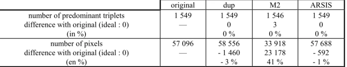
original dup M2 ARSIS number of predominant triplets
difference with original (ideal : 0) (in %) 1 549 — 1 5490 0 % 1 546 3 0 % 1 549 0 0 % number of pixels
difference with original (ideal : 0) (en %) 57 096 — 58 556 - 1 460 - 3 % 33 918 23 178 41 % 57 688 - 592 - 1 % Table 8. Performance in synthesizing the multispectral information. Difference between the actual
frequency of a triplet (XS1, XS2, XS3) and its estimate. Only the most frequent triplets are taken into account. The total of pixels they represent amounts to 22 percent of the total number of pixels in the image. Each triplet has a frequency of at least 26 pixels, i.e., at least 0.01 percent of the total number of pixels.
20 m 40 m
Bias (ideal value: 0) relative to the mean XS value
0.00 0 %
0.00 0 % Actual variance - estimate (ideal value: 0)
relative to the actual variance 5 %7 9 %12
Correlation coefficient between XS and estimate (ideal value: 1) 0.99 0.98
Standard-deviation of the differences (ideal value: 0) relative to the mean XS value
1.9 3 %
2.2 4 %
Table 9. Some statistics on the differences between the original and synthesized images (in radiance or relative value) for XS1 band.
0.001 1 2 5 10 20 50
20 m 27 28 63 92 99 100 100
40 m 23 24 56 88 99 100 100
Table 10. Probability (in percent) for having in a pixel a relative error less than or equal to the thresholds noted in the first row. The ideal value is 100 as early as the first threshold 0.001 percent. The relative errors are in absolute value and in percent. For XS1.