HAL Id: hal-01292481
https://hal-mines-nantes.archives-ouvertes.fr/hal-01292481
Submitted on 23 Mar 2016HAL is a multi-disciplinary open access archive for the deposit and dissemination of sci-entific research documents, whether they are pub-lished or not. The documents may come from teaching and research institutions in France or abroad, or from public or private research centers.
L’archive ouverte pluridisciplinaire HAL, est destinée au dépôt et à la diffusion de documents scientifiques de niveau recherche, publiés ou non, émanant des établissements d’enseignement et de recherche français ou étrangers, des laboratoires publics ou privés.
Integrating order acceptance decisions with flexible due
dates in a production planning model with
load-dependent lead times
Nadjib Brahimi, Tarik Aouam, El-Houssaine Aghezzaf
To cite this version:
Nadjib Brahimi, Tarik Aouam, El-Houssaine Aghezzaf. Integrating order acceptance decisions with flexible due dates in a production planning model with load-dependent lead times. In-ternational Journal of Production Research, Taylor & Francis, 2015, 53 (12), pp.3810-3822. �10.1080/00207543.2014.993045�. �hal-01292481�
Integrating order acceptance decisions with flexible due dates in a
production planning model with load-dependent lead times
Nadjib Brahimi
a, Tarik Aouam
b*, and El-Houssaine Aghezzaf
caDepartment of Industrial Engineering and Management
University of Sharjah, United Arab Emirates. nbrahimi@sharjah.ac.ae
bDepartment of Business Informatics and Operations Management, Faculty of Economics and
Business Administration, Ghent University Tweekerkenstraat 2, 9000 Gent, Belgium
Tarik.Aouam@ugent.be
cDepartment of Industrial Management, Faculty of Engineering and Architecture, Ghent
University
Technologiepark 903, 9052 Gent-Zwijnaarde, Belgium ElHoussaine.Aghezzaf@ugent.be
Abstract
We consider a tactical planning problem, which integrates production planning decisions together with order acceptance decisions, while taking into account the dependency between workload and lead times. The proposed model determines which orders to accept and in which period they should be produced so that they can be delivered to the customer within the acceptable flexible due dates. When the number of accepted orders increases, the workload and production lead time also increase and this may result in the possibility of missing customer due dates. This problem is formulated as a mixed integer linear program for which two relax-and-fix heuristic solution methods are proposed. The first one decomposes the problem based on time periods while the second decomposes it based on orders. The performances of these heuristics are compared with that of a state-of-the-art commercial solver. Our results show that the time-based relax-and-fix heuristic outperforms the order-based relax-and-fix heuristic and the solver solution as it yields better integrality gaps for much less CPU effort.
Keywords: Production Planning; Order Acceptance; Clearing Functions; Load-Dependent
2
1. Introduction
The usual production planning models have as primary objective customer demand satisfaction while minimizing production costs or maximizing profit. At the tactical level, customer orders are grouped as part of aggregation decisions that are made on data in order to either simplify the planning model or for managerial purposes (see Jacobs et al., 2011). However, it is often important to distinguish customer orders for several reasons (Pahl et al., 2007; Aouam and Brahimi, 2013). Firstly, even if the finished good is the same, different customers might impose particular conditions on the source of raw materials or on the quality control tests to be carried out during the manufacturing process of their orders. Secondly, in the case of limited capacity, the production planner can only satisfy demands partially and consequently has to decide which orders to satisfy.
Furthermore, even when there is enough capacity to avoid shortage, it is not always clear whether all orders should be accepted or not. Indeed, traditional production planning models make two fundamental assumptions: (i) the production lead times are constant and do not depend on the workload, (ii) and in any given period, the shadow price of the capacity constraint is equal to zero when there is enough capacity (capacity constraint is not binding); this means that the cost of adding one unit (or order) to the production stage is zero as long as the capacity limit is not reached. As a consequence of these assumptions, production planning models try to satisfy as many customer orders with known due dates as production capacity permits.
Production lead-times, i.e., the time required for material released into the production system to be transformed into finished goods that can be used to meet demand, depend on the workload. Queuing models have revealed that lead-time increases non-linearly as the resource utilization approaches 100% (Buzacott and Shanthikumar, 1993; Hopp and Spearman, 2001). This creates a circular, non-linear dependency between lead-time and utilization: production planning needs to be cognizant of times in making its release decisions, since the lead-times are a consequence of the workload, and hence the release decisions. Therefore, the more orders are accepted the higher are the production lead times, resulting in the possibility of missing customer due dates. This means that the planner can be faced with situations where production capacity is available but the next orders should be rejected in order not to delay some already accepted customer orders.
In addition, even if the unit price the customer is willing to pay exceeds the variable production cost and there is enough capacity to avoid shortage, the decision whether a customer order should be accepted or not is not always straightforward. There are two possible arguments to support this fact. The first argument has to do with economies of scale. In fact, in the case of high fixed or set-up costs it might not be economical to satisfy a single order of a small quantity. The order must be aggregated with additional orders to justify the production setup (Geunes et al., 2006). The second argument has to do with the workload of the production stage. Kefili et al. (2011) show that the marginal prices of capacitated resources are not necessarily equal to zero when the utilization is less than one. This means that even in the case where capacity is available, the revenue from an additional order should at least offset the variable production cost plus the shadow prices of the capacity constraints that take into account workload.
Therefore, models that integrate production planning decisions with load dependent lead times and order acceptance decisions have a great potential to improve the overall profitability of the firm. In addition, when due date flexibility is allowed, i.e., the due date required by the customer is given as an interval of possible dates (time window) rather than a fixed date, more orders can be accepted resulting in higher profits and more reliable delivery dates (lower delays). In this research work, we integrate order acceptance and production planning decisions in a single model, while considering flexible due dates and load dependent lead times. When an order is accepted, it is scheduled over a planning horizon of T periods and incurs production costs and eventually inventory holding costs. The rejection of a customer order results in a lost sale cost. To quantify the benefits of order acceptance integration, the proposed model is compared to a production planning model with load dependent lead-times where all orders are accepted resulting in backorders in the case of capacity shortage. Furthermore, to evaluate the benefits of flexibility, the proposed model is compared to an integrated production planning model with order acceptance considering fixed due dates and lost sales. The considered problem is formulated as a mixed integer linear program (MILP). When the number of orders and the number of periods increase, and for certain parameter settings it becomes difficult if not impossible to obtain good solutions in reasonable computation times. We propose relax-and-fix heuristics to solve efficiently large instances of the problem.
4
The remainder of the paper is organized as follows. A literature review is presented in Section 2. In section 3, the production planning problem with backordering where all orders are accepted is formulated. In section 4, order acceptance decisions are integrated with production decisions. Two models are then presented, one in which due dates are fixed and another one which considers flexible due dates. In section 5, two relax-and-fix heuristics are presented. Section 6 presents some numerical experiments to compare the three models economically and evaluate the proposed heuristics. Some concluding remarks are presented in Section 7.
2. Literature Review
The dependency between resource utilization and lead times (or equivalently available capacity) has already been addressed to some degree by some authors. Voss and Woodruff (2003) propose a nonlinear model where the function linking lead time to workload is approximated by a piecewise linear function. Ettl et al. (2000) take a similar approach, and added a convex term, representing the cost of carrying work-in-process (WIP) as a function of workload, to the objective function. Graves (1986), Karmarkar (1989), Missbauer (2002), and Asmundsson et al. (2006; 2009) use clearing functions (CFs) to model the dependency between workload and lead times. Several related models are proposed in the recent book by Hackman (2008). Pahl et al. (2005, 2007) and Missbauer and Uzsoy (2010) review production planning models with load-dependent lead times. Aouam and Uzsoy (2012; 2014) compare the performance of various production planning models with workload-dependent lead times under demand uncertainty. In this paper, a CF is used to model the capacity of the production stage in order to relate the production workload resulting from all accepted orders to the production lead-times.
Ivanescu et al. (2002) consider the order acceptance problem in the batch industries where the processing times are uncertain. The authors use regression based models in order to determine whether there is enough capacity to accept a customer order with the due date requested by the customer. Markov decision models are used by Defregger and Kuhn (2005) to decide about the orders to accept or to reject in a planning process over a number of periods. Geunes et al. (2002) consider a production planning problem with order acceptance and call it the order selection problem. The uncapacitated case is solved using a polynomial time algorithm and they propose a Lagrangian relaxation approach for the capacitated case. For a more extensive review of order acceptance literature the reader is referred to Slotnick (2011). Aouam and Brahimi (2013) present a robust model that integrates production
planning with load dependent lead-times and order acceptance decisions, which considers demand uncertainty and where a fraction of the order quantity can be accepted. They show that integrating the two decisions provides the planner with the flexibility to select the orders to be satisfied fully or partially. This flexibility enables the planner to maintain release quantities and utilization at desirable levels, which leads to high profits and high levels of customer satisfaction. Unlike their work, the present paper accepts to deliver the entire quantity of an order or none and hence order acceptance/rejection decisions are modeled as binary variables. Furthermore, the present paper considers customer due date flexibility.
The subject of lead time or due date flexibility is directly related to demand time windows. The latter are grace periods (allowed by the customers) during which the order can be delivered without penalty. To the best of our knowledge, the first production planning models with demand time windows were introduced by Lee et al. (2001). They proposed dynamic programming algorithms to solve uncapacitated lot sizing problems with and without backlogging. Charnsirisakskul et al. (2004) propose an order acceptance model where they show the economic benefits of lead time flexibility. They solve a capacitated example using the commercial solver CPLEX. Merzifonluoğlu and Geunes (2006) propose a similar model with production setup decisions. The uncapacitated case is solved using a dynamic programming algorithm, while the authors propose heuristics to solve the general case. This stream of work emphasizes the integration of order acceptance decisions in production planning decisions to take into account economies of scale achieved per setup when orders are aggregated. Recently, Brahimi (2014) considered the issue of integrating order acceptance decisions with due date flexibility. He presents two heuristic solutions for the problem: a reversals heuristic and a relax-and-fix heuristic based on order decomposition. The present paper improves these heuristics and presents a new time based relax and fix heuristic that outperforms them in terms of integrality gap and CPU times. This paper also analyses the effects of workload and shows that there is added value from integrating order acceptance and due date flexibility in production planning models.
Relax-and-fix heuristics were applied to different production planning problems including the capacitated single level multi-item lot sizing problem (Federgruen et al. 2007), the multi-level lot sizing problem (Stadtler, 2003), and the lot sizing and scheduling problem with parallel machines (Beraldi et al., 2008). It was also used to solve problems in particular applications. Toso et al. (2009), for example, solve a lot sizing problem at an animal-feed
6
plant using three different variants of a relax-and-fix heuristic. Ferreira et al. (2010) use the embedded relax-and-fix heuristic of commercial solver CPLEX to solve a production planning problem that arises in soft drink plants. Relax-and-fix heuristics consist of fixing different sub-categories of variables and relaxing the others (ex. Toso, 2009). Most implementations in production planning consider partitioning the time horizon and forward or backward fixing integer variables (ex. Federgruen and Tzur, 1999; Stadtler, 2003; Federgruen et al. 2007; and Akartunali and Miller, 2009).
Compared to previous work, our models consider more realistic capacity constraints that reflect the dependency between workload, affected by the number of accepted orders, and production lead times. The models also incorporate flexible due dates that allow production smoothing, increase the number of accepted orders, and determine reliable due dates. Furthermore, two relax and fix heuristics are proposed and compared: one decomposes the problem based on time periods and the other based on customer orders. The latter heuristic incorporates reversals, which are inspired by the sub-tour reversals heuristic for the traveling salesman problem (Taha, 2010).
3. Production Planning With Load-Dependent Lead Times
Linear programming based production planning models typically consider fixed lead times or time lags and represent capacity as a fixed upper bound on the number of hours available at the resource in a period (Voss and Woodruff, 2003). However, these lead times or time lags are independent of workload. As an alternative, load-dependent production planning models with clearing functions (CFs) capture the relationship between workload and output at a capacitated production resource (Graves, 1986; Srinivasan et al., 1988; Karmarkar, 1989). A CF represents the relationship between the average workload of a production resource, usually some measure of work in process inventory (WIP), and the average throughput of the resource in a planning period. For most capacitated production resources subject to congestion, limited capacity leads to a CF that is concave and increasing (Missbauer and Uzsoy, 2010).
The load-dependent production planning model determines production decisions to match aggregate demand in each period in order to maximize the total profit. Customer orders in this case are aggregated based on their delivery due date. Each order 𝑖 is characterized by an order size 𝑞𝑖, reservation price or marginal revenue 𝜋𝑖 and a due date 𝜏𝑖. Orders can be delayed as
model are, for each period: the quantity released 𝑅𝑡, the production level 𝑋𝑡, the Work-In-Process (WIP) level 𝑊𝑡, the inventory level 𝐼𝑡, and the backlogging level 𝐵𝑡. The marginal costs are: release cost 𝑟𝑡, processing cost 𝑐𝑡, WIP holding cost 𝑤𝑡, inventory holding cost ℎ𝑡, and backlogging cost 𝑝𝑡. The CF, denoted by 𝑓(. ) that is increasing and concave with 𝑓(0) = 0, relates the throughput to the WIP as follows,
𝑋𝑡 = 𝑓(𝑊̅𝑡) ∀𝑡 (1)
where 𝑊̅𝑡 = 𝑊𝑡−1+ 𝑅𝑡 represents the resource load for period t, or the total amount of work
that becomes available for processing during the period. Following Asmundsson et al. (2006) and Missbauer (2002), and for tractability reasons, the CF is approximated using an outer linearization. In fact, 𝑓(. ) can be approximated by the convex hull of a set of affine functions of the form,
𝑓̂(𝑊) = 𝑚𝑖𝑛𝑘=1…𝐾{𝑎𝑘𝑊 + 𝑏𝑘} (2)
𝑎𝑘 and 𝑏𝑘 are the slope and intercept of the segments 𝑘 ∈ {1 … 𝐾}. The load-dependent
production planning model is given by:
PP-B Objective function: 𝑀𝑎𝑥𝑖𝑚𝑖𝑧𝑒 𝑃𝐵(𝑅 𝑡, 𝑋𝑡, 𝑊𝑡, 𝐼𝑡, 𝐵𝑡) = ∑ 𝜋𝑖𝑞𝑖 𝑖 − ∑(𝑟𝑡𝑅𝑡+ 𝑐𝑡𝑋𝑡+ 𝑤𝑡𝑊𝑡+ ℎ𝑡𝐼𝑡+ 𝑝𝑡𝐵𝑡) 𝑡 (3) Subject to constraints: 𝑊𝑡 = 𝑊𝑡−1+ 𝑅𝑡− 𝑋𝑡 𝑡 = 1, . . . , 𝑇 (4) 𝐼𝑡 = 𝐼𝑡−1+ 𝑋𝑡− ∑ 𝑞𝑖 {𝑖: 𝜏𝑖=𝑡} + 𝐵𝑡− 𝐵𝑡−1 𝑡 = 1, . . . , 𝑇 (5) 𝑋𝑡 ≤ 𝑎𝑘(𝑊𝑡−1+ 𝑅𝑡) + 𝑏𝑘 𝑡 = 1, . . . , 𝑇 ∧ 𝑘 = 1, . . . , 𝐾 (6) 𝑅𝑡, 𝑋𝑡, 𝑊𝑡, 𝐼𝑡, 𝐵𝑡≥ 0 𝑡 = 1, . . . , 𝑇 (7)
The objective function in equation (3) maximizes the total profit 𝑃𝐵 over the planning horizon. Constraints (4) and (5) define WIP and finished goods inventory balances, respectively for each period. Constraints (6) represent the capacity constraints defined by the CF. The non-negativity constraints are defined in (7).
4. Integrated Production Planning Models with Order Acceptance
In the PP-B model, as the number of orders increases the WIP also increases leading to elongated production lead times. This can result in backorders, i.e., some orders might be
8
delivered after their due dates. Therefore, giving the production planner the flexibility to accept or reject orders would lead to higher profitability for the firm. This can be achieved by integrating order acceptance and production planning decisions in a single model. Let the binary variable 𝑌𝑖 such that 𝑌𝑖 = 1 if order i is accepted and 𝑌𝑖 = 0 otherwise. The marginal cost of lost sale corresponding to order i is denoted by 𝑙𝑖. The integrated production planning
model with order acceptance is formulated as follows:
PP-OA Objective function: 𝑀𝑎𝑥𝑖𝑚𝑖𝑧𝑒 𝑃𝑂𝐴(𝑅 𝑡, 𝑋𝑡, 𝑊𝑡, 𝐼𝑡, 𝑌𝑖) = ∑ 𝜋𝑖𝑞𝑖𝑌𝑖 𝑖 − ∑(𝑟𝑡𝑅𝑡+ 𝑐𝑡𝑋𝑡+ 𝑤𝑡𝑊𝑡+ ℎ𝑡𝐼𝑡) 𝑡 − ∑ 𝑙𝑖(1 − 𝑌𝑖) 𝑖 (8) Subject to constraints: 𝑊𝑡 = 𝑊𝑡−1+ 𝑅𝑡− 𝑋𝑡 𝑡 = 1, . . . , 𝑇 (9) 𝐼𝑡 = 𝐼𝑡−1+ 𝑋𝑡− ∑ 𝑞𝑖𝑌𝑖 {𝑖: 𝜏𝑖=𝑡} 𝑡 = 1, . . . , 𝑇 (10) 𝑋𝑡 ≤ 𝑎𝑘(𝑊𝑡−1+ 𝑅𝑡) + 𝑏𝑘 𝑡 = 1, . . . , 𝑇 ∧ 𝑘 = 1, . . . , 𝐾 (11) 𝑅𝑡, 𝑋𝑡, 𝑊𝑡, 𝐼𝑡 ≥ 0 𝑡 = 1, . . . , 𝑇 (12) 𝑌𝑖: 𝑏𝑖𝑛𝑎𝑟𝑦 𝑖 = 1, . . . , 𝑁 (13)
The objective function in equation (8) maximizes the total profit 𝑃𝑂𝐴 over the planning horizon. The first term is the revenue generated from the orders accepted, the second term is the total production costs, and the last term is the total cost of lost sales. Constraints (10) are the modified finished goods inventory balance. The other constraints are as defined above.
The previous model takes into account load dependent lead-times in order to ensure that delivery of accepted orders meets the pre-specified due dates. This model however, can result in a high number of rejected orders. When due date flexibility is allowed, i.e., the due date required by the customer is given as a set of possible dates rather than a fixed date, a win-win situation for the firm and customers can be achieved. In fact, this flexibility when captured in production planning models results in more accepted orders, smoother production plans, higher profits, and more reliable due dates (lower delays). In this setting, a customer provides a time window with earliest delivery date 𝑒𝑖 and a latest delivery date 𝑓𝑖. Let the binary
𝑆𝑖𝑡 = 0 otherwise. The integrated production planning and order acceptance model with flexible due dates can be formulated as follows:
PP-OA-FDD Objective function: 𝑀𝑎𝑥𝑖𝑚𝑖𝑧𝑒 𝑃𝐹𝐷𝐷(𝑅 𝑡, 𝑋𝑡, 𝑊𝑡, 𝐼𝑡, 𝑆𝑖𝑡) = ∑ 𝜋𝑖𝑞𝑖 ∑ 𝑆𝑖𝑡 𝑓𝑖 𝑡=𝑒𝑖 𝑖 − ∑(𝑟𝑡𝑅𝑡+ 𝑐𝑡𝑋𝑡+ 𝑤𝑡𝑊𝑡+ ℎ𝑡𝐼𝑡) 𝑡 − ∑ 𝑞𝑖𝑙𝑖(1 − ∑ 𝑆𝑖𝑡 𝑓𝑖 𝑡=𝑒𝑖 ) 𝑖 (14) Subject to constraints: 𝑊𝑡 = 𝑊𝑡−1+ 𝑅𝑡− 𝑋𝑡 𝑡 = 1, . . . , 𝑇 (15) 𝐼𝑡 = 𝐼𝑡−1+ 𝑋𝑡− ∑ 𝑞𝑖𝑆𝑖𝑡 𝑖 𝑡 = 1, . . . , 𝑇 (16) 𝑋𝑡 ≤ 𝑎𝑘(𝑊𝑡−1+ 𝑅𝑡) + 𝑏𝑘 𝑡 = 1, . . . , 𝑇 ∧ 𝑘 = 1, . . . , 𝐾 (17) ∑ 𝑆𝑖𝑡 𝑓𝑖 𝑡=𝑒𝑖 ≤ 1 𝑖 = 1, . . . , 𝑁 (18) 𝑅𝑡, 𝑋𝑡, 𝑊𝑡, 𝐼𝑡, ≥ 0 𝑡 = 1, . . . , 𝑇 (19) 𝑆𝑖𝑡: 𝑏𝑖𝑛𝑎𝑟𝑦 𝑡 = 1, . . . , 𝑇 ∧ 𝑖 = 1, . . . , 𝑁 (20) The objective function in equation (14) maximizes the total profit 𝑃𝐹𝐷𝐷 over the planning horizon. Constraints (18) ensure that order i can only be accepted and satisfied within the customer specified time window [𝑒𝑖, 𝑓𝑖].
5. Heuristics for Solving PP-OA-FDD
5.1 General structure of the heuristics
For problems of realistic sizes, with a large number of planning periods and orders, problem PP-OA-FDD is very hard to solve in reasonable computational times. This section presents two relax-and-fix heuristics to tackle this difficulty. The first heuristic decomposes the problem based on time periods while the second decomposes the problem based on customer orders. In relax-and-fix heuristics, the integer variables in a MILP formulation are separated into subsets. The heuristic usually proceeds by fixing a subset of variables, usually the most important ones, and relaxing the integrality of the other variables. Then, it gradually fixes the
10
relaxed variables (Wolsey, 1998). A very detailed and practical presentation of a relax-and-fix heuristic for lot sizing problems can be found in Pochet and Wolsey (2006). The only integer/binary variables in PP-OA-FDD formulation are 𝑆𝑖𝑡 variables and thus the problem can be decomposed over orders (𝑖 = 1. . 𝑁) or over time periods (𝑡 = 1. . 𝑇).
5.2 Time-based relax-and-fix heuristic
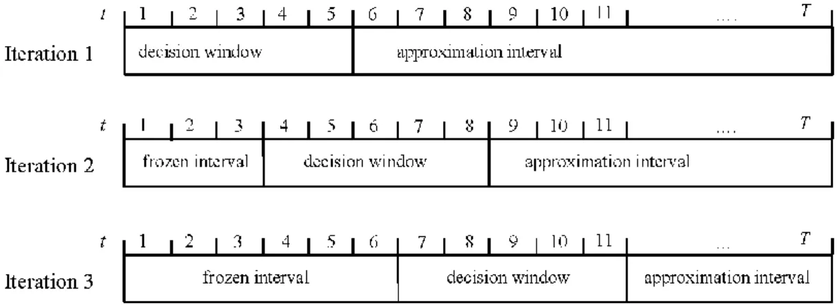
In the time based decomposition, integrality constraints are imposed on variables 𝑆𝑖𝑡 (∀ 𝑖 = 1. . 𝑁) within a decision time window, which is an internally rolling horizon. In any iteration of the relax-and-fix heuristic, the time horizon (the set of decisions over the time horizon) is partitioned into three intervals (subsets of variables): a decision time window (integer decision subset), a frozen interval (frozen subset) preceding the decision time window and consisting of periods with variables that are fixed, and an approximation interval (relaxed subset) after the decision window where the binary constraints are relaxed. The two main parameters of this approach are: the size of the decision time window (𝛼) and the size of the frozen interval (𝛽 ≤ 𝛼). In any iteration, the decisions of the first 𝛽 periods in the current decision window will be frozen in the following iteration. Figure 1 illustrates the three sub-intervals for 𝛼 = 5 and 𝛽 = 3. In each iteration, an optimal or heuristic solution is obtained using a MILP solver. If the heuristic approach is adopted, then two stopping parameters need to be determined for the heuristic: the minimum integrality gap and the maximum allowed CPU time in each iteration.
Figure 1. The different intervals in a time-based decomposition of a relax-and-fix heuristic
5.3 Order-based relax-and-fix heuristic
The main difference between the order-based decomposition and the time-based decomposition is that intervals (subsets of decisions) are naturally identified because of the chronological nature of time periods, while a sequence of orders (𝐼 = {𝑖1, 𝑖2, … , 𝑖𝑁}) needs to
given feasible solution of the problem instance. Several sequences of orders are constructed and evaluated.
An initial sequence is obtained using a Most Profitable First (MPF) priority rule. In the MPF rule, initially, all orders are supposed to be released and satisfied on their earliest due date, which yields a unit profit of 𝜋𝑖′ = 𝜋𝑖 − 𝑟(𝜏𝑖) for each order 𝑖 and the sequence (𝐼 =
{𝑖1, 𝑖2, … , 𝑖𝑁}) is obtained by sorting the orders in decreasing order of unit profit 𝜋𝑖′
using QuickSort function as shown on line 10 of Algorithm 1. For this sequence, the relax-and-fix heuristic is applied in such a way that the decision subset corresponds to the first 𝛼′ orders.
The frozen subset is 𝛽′≤ 𝛼′ (line 180) and the decisions corresponding to the rest of the orders belong to the relaxed subset.
After updating the best solution (line 200), other sequences are constructed using the reversals heuristic, subroutine Reverse. When the initial sequence is reversed two-by-two, the resulting new sequences are: 𝐼 = {𝑖2, 𝑖1, … , 𝑖𝑁}, 𝐼 = {𝑖1, 𝑖3, 𝑖2, … , 𝑖𝑁}, …, 𝐼 = {𝑖1, 𝑖2, … , 𝑖𝑁, 𝑖𝑁−1}. The best reversal and solution value are saved. The best sequence in the two-by-two reversal is used as a starting point for a three-by-three reversal. Supposing that the best solutions obtained for sequence {𝑖1, 𝑖3, 𝑖2, 𝑖4, 𝑖5, … , 𝑖𝑁} in the two-by-two reversals, in the three-by-three
reversals, the generated sequences are {𝑖2, 𝑖3, 𝑖1, 𝑖4, 𝑖5, … , 𝑖𝑁}, {𝑖1, 𝑖4, 𝑖2, 𝑖3, 𝑖5, … , 𝑖𝑁},
{𝑖1, 𝑖3, 𝑖5, 𝑖4, 𝑖2, … , 𝑖𝑁}, …, and {𝑖1, 𝑖3, 𝑖2, 𝑖4, 𝑖5, … , 𝑖𝑁, 𝑖𝑁−1, 𝑖𝑁−2}. The best sequence in the three-by-three reversals is the starting point of a four-by-four reversals and so on.
12
The Relax-and-fix(𝛼′, 𝛽′) subroutine (Algorithm 2) forces the integrality condition on binary variables of the first 𝛼′ orders with the highest profit 𝜋′ and relaxes the other binary variables. Then, it permanently fixes the solution for the first 𝛽′ variables (𝛽′ ≤ 𝛼′), sets
integrality constraints on variables indexed from 𝛽′+ 1 to 𝛽′+ 𝛼′ and relaxes integrality
for orders after 𝛽′+ 𝛼′ + 1. The process is repeated until the last order in the sorted list is
reached. Furthermore, compared to simple relax-and-fix heuristics, our heuristic applies the reversals function and explores more possible solutions. The heuristic’s main inputs are the number of orders for which the integrality constraints are to be respected in each iteration (𝛼′) and the number of orders for which the binary variables are to be permanently fixed in each iteration (𝛽′). The first step of the heuristic calculates the number of iterations based on these two parameters. Then, starting from the beginning of the sequence of the sorted orders, the sub-problems are solved until all binary decision variables are fixed.
Algorithm 1: RerversalsHeuristic
BestSequence ← QuickSort(Orders); BestProfit ← −∞
for Reversals ← 1 until N do if Reversals = 1 then MaxReversals ← 1 else MaxReversals ← N-Reversals+1 end-if ReversalBestProfit ← −∞
for ReversePoint ← 1 until MaxReversals do
for i ← 1 until N do S[i] ← 0; flag ← true; if (Reversals > 1) then Reverse(BestSequence,ReversePoint,ReversePoint+Reversals-1) end-if SequenceBestProfit ← −∞ Relax-and-fix(𝛼′, 𝛽′, sequence)
if (SequenceBestProfit ≥ ReversalBestProfit) then
ReversalBestProfit ← SequenceBestProfit; UpdateBestSequence();
end-if
end-for
if (ReversalBestProfit ≥ BestProfit) then
BestProfit ← ReversalBestProfit; UpdateBestSequence();
end-if
6. Experimental Results
This section evaluates the added value from integrating production and order acceptance decisions and introducing due date flexibility. It also evaluates the efficiency of the proposed heuristics. The optimization models as well as the heuristics have been implemented in Xpress-IVE version 1.24 (2013) and run on a PC with intel CORE i7-2.4Ghz microprocessor and 16GB RAM.
6.1. Generated data sets
Two groups of data sets were generated. A first group with 𝑇 = 8 and 𝑁 = 15 was generated to carry out the economic experiments (Section 6.2) and a second group corresponding to a total of 𝑁 =20 to 500 orders received for a period of 𝑇 =10 to 100 periods. The production related unit costs are 𝑟𝑡 =$3, while 𝑐𝑡 =0, 𝑤𝑡 =$35, and ℎ𝑡=$15,
∀𝑡. The unit profit is equal to 100, 110 and 115 for small, medium, and large size orders, respectively. The earliest delivery date of each order is generated from a uniform distribution between 1 and 𝑇. The size of each order is generated from a uniform distribution between 1
2𝑞̅
and 32𝑞̅, where:
𝑞̅ =𝑇 × 𝑏𝐾× 𝐷𝐶 𝑁
𝐷𝐶 is the total orders over the nominal capacity for the whole planning horizon, i.e. 𝐷𝐶 =
∑ 𝑞𝑖 𝑖
𝑇×𝑏𝐾.
The lost sale cost per unit is: 𝑙𝑖 = 1.2 × 𝜋𝑖. The intercepts and the slopes of the clearing function are defined as (𝑎𝑘, 𝑏𝑘) = (0.5, 0), (0.069, 136), (0.036, 154.8), (0, 180) for 𝑘 =
1, . . . ,4. In the case of PP-B model, the penalty cost 𝑝𝑡 = 8 × ℎ𝑡. The analysis of the effectiveness of the models and the performance of the heuristics was based mainly on capacity tightness determined by coefficient 𝐷𝐶 = 𝑇×𝑏∑ 𝑞𝑖 𝑖
𝐾 and order time window Δ𝑖 = 𝑓𝑖 −
𝑒𝑖+ 1. DC was varied between 0.6 (loose capacity) and 1.2 (demand exceeding capacity). To
Algorithm 2: Subroutine Relax-and-Fix(𝛼′, 𝛽′, Sequence)
Input: 𝛼′, 𝛽′
Caculate NumIter for i ← 1 until NumIter
Relax binary variables of orders after the last 𝛼′ interval
Solve the sub-problem Permanently fix 𝑆𝑖𝑡 variables for orders within 𝛽′
14
analyze the impact of due date flexibility, Δ𝑖 was varied between 1 and 6, where Δ𝑖 = 1 corresponds to PP-OA model, while Δ𝑖 > 1 corresponds to PP-OA-FDD model.
6.2. Economic experiments
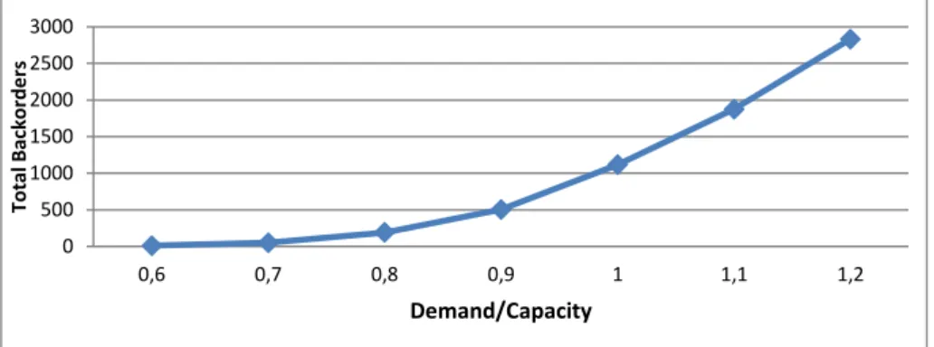
The effectiveness of the proposed integrated model PP-OA-FDD is shown by comparing its performance in terms of profit and fraction of accepted orders with those of B and PP-OA models. The numerical tests are carried out on problems with 𝑇 = 8 and 𝑁 = 15 for which optimal solutions are obtained using Xpress solver. Figure 2 shows the total amount of backorders when PP-B model is used. As can be noticed, as demand gets closer to or larger than the total available capacity, the total backorders increase rapidly. Though, from the sales perspective, accepting all orders certainly generates more revenue, the cost of backorders and excessive delays increases considerably resulting in a decrease in profits. This is depicted in Figure 3, which shows the total profit of the three models (PP-B, PP-OA, and PP-OA-FDD) as a function of the ratio Demand/Capacity (DC). It is interesting to notice how fast the profit is decreasing for model PP-B, though the revenue increases linearly with DC (as demand is increased). Between PP-OA and PP-OA-FDD (Δ𝑖 = 3) models, the effect of flexibility is more remarkable especially for higher DC values; for example, in the case of DC=1.2, the profit in PP-OA-FDD model is double the profit of PP-OA model.
Figure 2. Backorders vs. capacity tightness
0 500 1000 1500 2000 2500 3000 0,6 0,7 0,8 0,9 1 1,1 1,2 Tot al Back order s Demand/Capacity -250000 -200000 -150000 -100000 -50000 0 50000 100000 150000 0,6 0,7 0,8 0,9 1 1,1 1,2 Pr o fi t Demand/Capacity PP-B PP-OA PP-OA-FDD
Figure 3. Total profit of the three models (Δi =3 in PP-OA-FDD)
The increase in the profit of PP-OA-FDD is due to the increase in accepted orders as flexibility is introduced (See Figure 4 and Figure 5).
Figure 4. Accepted orders with and without due date flexibility (Δi =3 in PP-OA-FDD)
Figure 5. Fraction of accepted orders for PP-OA and PP-OA-FDD (Δ =1 corresponds to PP-OA model)
6.3 Analysis of the performance of the heuristics
The PP-OA-FDD model was solved using the time-based relax-and-fix heuristic and using order-based relax-and-fix heuristic (Algorithm 1). The parameters used for each heuristic are summarized in Table 1. The numerical experiments were carried on both small size and large size instances. The stopping criterion used in each iteration of the two heuristics is the minimum integrality gap, which is set to 0.1%.
Table 1. Parameters of the heuristics
0,6 0,7 0,8 0,9 1 1,1 0,6 0,7 0,8 0,9 1 1,1 1,2 Fr ac ti o n o f A cc e p te d O rd e rs Demand/Capacity PP-OA PP-OA-FDD 0,6 0,65 0,7 0,75 0,8 0,85 0,9 0,95 1 1,05 1 2 3 4 5 6 Fr ac ti o n o f A cc e p te d O rd e rs Δi DC=0.6 DC=0.9 DC=1.2
16
Order-based heuristic Time-based heuristic RF-N-10-8 RF-N-15-10 RF-T-5-3 RF-T-10-8
𝛼 10 15 5 10
𝛽 8 10 3 8
Min integrality gap 0.1% 0.1% 0.1% 0.1%
Preliminary tests were carried out on small size problems. In these problems there are 𝑁 = 20 orders to be scheduled over a planning horizon of 𝑇 = 10 periods. Order time windows were set to Δ𝑖 ∈ {2, 4, 6} and capacity tightness was set to 𝐷𝐶 ∈ {0.6, 0.9, 1.2}. For each setting (given values of Δ𝑖 and 𝐷𝐶), five instances were randomly generated as mentioned in Section 6.1. The performance of the heuristics is measured using the gap between the optimal solution (𝑂𝑝𝑡) obtained using the solver and the heuristic solution (𝑆𝑜𝑙):
𝐺𝑎𝑝 = 100 ×𝑂𝑝𝑡 − 𝑆𝑜𝑙 𝑂𝑝𝑡
Table 2 shows the gaps obtained by the heuristics. The CPU times are shown on the last raw of the table.
Table 2. Gaps and CPU times for small size problems (𝑇 = 10, 𝑁 = 20)
Parameter Value RF-N-10-8 RF-N-15-10 RF-T-5-3 RF-T-10-8 Gap (%) Δ 𝑖 2 1.09 0.36 0.46 0.00 4 1.80 0.40 0.16 0.01 6 2.02 0.39 0.19 0.01 DC 0.6 0.14 0.15 0.06 0.02 0.9 0.46 0.16 0.18 0,00 1.2 4.30 0.84 0,57 0,00 CPU (Seconds) 0.70 0.82 0.31 2.57
The RF-T-10-8 heuristic outperforms all other heuristics in terms of quality of solutions. In fact, for some parameter settings it is able to find the optimal solutions for all the generated instances. However, it requires the largest CPU time on average when compared to other heuristics. Heuristic RF-T-5-3 might be considered as a good compromise between CPU time and solution quality. The solver on the other hand requires an average CPU time of 6.25 seconds and a maximum CPU time of 900 Seconds (maximum allowed execution time) to find the optimum, while RF-T-10-8 heuristic requires an average time of 2.57 Seconds and a maximum time of 97 Seconds to reach an average gap of 0.01 %.
a) Full factorial tests
In Table 3, the first and second columns correspond to the three problem parameters and their values based on which the analysis was done. Problem size is identified by the number of time periods in the planning horizon and the number of orders (T-N), which range from 10 to 100 periods and from 20 to 500 orders. The execution time of the solver when applied directly to the PP-OA-FDD formulation was limited to 900 Seconds. The last six columns in Table 3 present the average solution gap of two order-based relax-and-fix heuristics, two time-based relax-and-fix heuristics and the solver for a maximum CPU time of 900 Seconds (Column Solver 900s).
Gap' = 100 ×𝐵𝑒𝑠𝑡𝑈𝐵 − 𝑆𝑜𝑙 𝑆𝑜𝑙
Where 𝑆𝑜𝑙 is the solution obtained using the solution approach and 𝐵𝑒𝑠𝑡𝑈𝐵 is the best bound obtained using the solver. We also refer to Table 4 for a comparison of the average CPU times.
As it can be expected, from Table 3, the solver provides better quality solutions than the heuristics for very small problems though it requires much more CPU times on average. For medium and large instances, the time-based relax-and-fix heuristics (RF-T-5-3 and RF-T-10-8) outperform the solver in terms of solution quality while requiring much less CPU time. For example, for problems with (𝑇, 𝑁) = (100,200), the solver requires 630 seconds to reach an average gap of 4.05%, while RF-T-5-3 obtains solutions with an average gap of 1.99% in less than 12 Seconds on average.
For problems with a large number of orders, the order-based relax-and-fix heuristics are slower than the time-based heuristics as the number of sequences to be evaluated becomes large. The main reason behind constructing and evaluating several sequences is to search for sequences that would result in good quality solutions; yet, it can be seen from Table 3 that order-based heuristics results in relatively higher gaps when compared to the solver and time-based heuristics. Therefore, the time-time-based relaxed and fix heuristics are more suitable for solving this problem.
It can also be seen from Table 5 that the more customer due date flexibility is allowed (increasing Δ𝑖) and the tighter is the capacity (increasing DC), the harder is the problem to solve.
18
Table 3. Gaps (%) between the best bound and the best solution of the heuristics
RF-N-10-8 RF-N-15-10 RF-T-5-3 RF-T-10-8 Solver900s T-N 10-20 1.63 0.38 0.27 0.01 0.00 10-50 0.85 0.68 0.11 0.09 0.05 20-40 1.94 1.47 0.55 0.51 0.35 20-60 1.81 1.49 0.58 0.51 0.55 10-100 0.96 0.83 0.14 0.15 0.09 20-100 1.77 1.39 0.36 0.31 0.37 50-100 3.74 3.21 1.59 1.44 2.58 50-300 4.23 3.57 0.64 0.66 1.23 100-200 5.68 5.01 1.99 1.89 4.05 100-500 7.40 5.94 0.99 0.83 1.74
Table 4. Average CPU time (in Seconds) for different problem sizes.
T-N RF-N-10-8 RF-N-15-10 RF-T-5-3 RF-T-10-8 Solver900 10-20 0.70 0.82 0.31 2.57 6.25 10-50 1.01 1.02 3.20 18.32 159.56 20-40 1.74 2.68 0.99 6.22 198.08 20-60 2.28 2.63 1.81 11.84 295.79 10-100 2.60 2.18 4.56 29.48 402.95 20-100 3.21 3.02 4.26 18.24 426.13 50-100 8.51 8.46 4.25 19.63 520.39 50-300 43.61 32.64 12.68 28.94 601.06 100-200 31.18 33.38 11.32 22.94 630.62 100-500 144.75 133.80 11.19 26.19 602.48
Table 5. Effect of Δ𝑖 and DC on Gaps
RF-N-10-8 RF-N-15-10 RF-T-5-3 RF-T-10-8 Solver900s Δ𝑖 2 3.18 2.24 0.54 0.37 0.44 4 3.06 2.50 0.74 0.64 1.05 8 3.69 3.25 1.12 1.11 2.09 12 4.77 4.38 1.44 1.47 3.23 DC 0.6 0.69 0.43 0.14 0.13 0.00 0.9 2.30 1.82 0.54 0.38 0.49 1.2 6.81 5.67 1.69 1.61 3.27 7. Conclusion
Integrating production and sales decisions increases the competitiveness of manufacturing firms. In fact, by integrating production planning and order acceptance decisions companies can increase profit and in the same time customer satisfaction, by
controlling delays and reducing them. Furthermore, negotiating flexible due dates allows companies to accept more orders and quote more reliable due dates to their customers. In this paper, we have proposed a mathematical programming formulation to model the integrated problem of production planning with load-dependent lead times, order acceptance, and flexible due dates. We quantified, through numerical experiments, the benefits of integration and due dates flexibility. For problems of realistic sizes, with a large number of planning periods and orders, the problem is very hard to solve in reasonable computational times. Therefore, two relax-and-fix heuristics have been developed to tackle this issue of dimensionality. Numerical results show that the time-based relax-and-fix heuristics outperform the order-based relax-and-fix heuristics and the direct application of a commercial solver as it provides better quality solutions in much less CPU times. Although the model presented in this paper considers more realistic behaviour of the capacity constraints, it still needs further improvements by considering other important issues related to production planning decisions such as setup costs, setup times and multi-products. Furthermore, faster solution approaches, which do not rely on the solution on integer linear programming problems need to be tackled and are currently under investigation.
8. References
Akartunali, K., and Andrew J. M. “A Heuristic Approach for Big Bucket Multi-level Production Planning Problems.” European Journal of Operational Research 193, no. 2 (2009): 396–411.
Aouam, T., and N. Brahimi. “Integrated Production Planning and Order Acceptance Under Uncertainty: A Robust Optimization Approach.” European Journal of Operational Research 228, no. 3 (2013): 504–515.
Aouam, T. and R. Uzsoy (2012). Chance-Constraint-Based Heuristics for Production Planning in the Face of Stochastic Demand and Workload-Dependent Lead Times. Decision Policies for Production Networks. K. G. Kempf and D. Armbruster. Boston, Springer: 173-208.
Asmundsson, J. M., R. L. Rardin, C. H. Turkseven and R. Uzsoy. "Production Planning Models with Resources Subject to Congestion." Naval Research Logistics 56 (2009): 142-157.
Asmundsson, J. M., R. L. Rardin and R. Uzsoy. "Tractable Nonlinear Production Planning Models for Semiconductor Wafer Fabrication Facilities." IEEE Transactions on Semiconductor Manufacturing 19 (2006): 95-111.
Beraldi, Patrizia, Gianpaolo Ghiani, Antonio Grieco, and Emanuela Guerriero. “Rolling-horizon and Fix-and-relax Heuristics for the Parallel Machine Lot-sizing and Scheduling Problem with Sequence-dependent Set-up Costs.” Computers & Operations Research 35, no. 11 (2008): 3644–3656.
Buzacott, John A., and J. George Shanthikumar. Stochastic Models of Manufacturing Systems. Prentice Hall, 1993.
Brahimi, N. “A Relax-and-Fix Heuristic for a Production Planning Problem with Order Acceptance and Flexible Due Dates”. Proceedings of the 2014 International Conference
20
on Industrial Engineering and Operations Management, Bali, Indonesia, January 7 – 9, 2014
Charnsirisakskul, Kasarin, Paul M. Griffin, and Pinar Keskinocak. “Order Selection and Scheduling with Leadtime Flexibility.” IIE Transactions 36, no. 7 (2004): 697–707. doi:10.1080/07408170490447366.
Defregger, F. and Kuhn, H., Markov Decision Models for Order Acceptance/Rejection Problems, in: : Fifth International Conference on Analysis of Manufacturing Systems – Production Management, May 2005, S. 265-272,
Ettl, M., G. Feigin, G. Y. Lin and D. D. Yao. "A Supply Chain Network Model with Base-Stock Control and Service Requirements." Operations Research 48 (2000): 216-232. Federgruen, A., J. Meissner, and M. Tzur. “Progressive Interval Heuristics for Multi-Item
Capacitated Lot-Sizing Problems.” Operations Research 55, no. 3 (2007): 490–502. Federgruen, Awi, and Michal Tzur. “Time-partitioning Heuristics: Application to One
Warehouse, Multiitem, Multiretailer Lot-sizing Problems.” Naval Research Logistics (NRL) 46, no. 5 (1999): 463–486.
Geunes, J., Taaffe, K., Romeijn, H.E. Models for integrated production planning and order selection. In: Proceedings of the 2002 Industrial Engineering Research Conference (IERC). Orlando (2002)
Geunes, J., Romeijn, H.E., and Taaffe, K.. Requirements planning with pricing and order selection flexibility. Operations Research, 54, no. 2 (2006): 394–401.
Graves, S. C.. "A Tactical Planning Model for a Job Shop." Operations Research 34 (1986): 552-533.
Hackman, Steven T. Production Economics: Integrating the Microeconomic and Engineering Perspectives. Springer, 2008.
Hopp, W. J. and M. L. Spearman. Factory Physics : Foundations of Manufacturing Management. Boston, Irwin/McGraw-Hill, 2001.
Ivanescu, C.V., Fransoo, J.C., and Bertrand, J.M., Makespan estimation and order acceptance in batch process industries when processing times are uncertain. OR Spectrum 24(4), (2002): 467-495.
Jacobs, F. Robert, Berry, William, Whybark, D. Clay, Vollmann, Thomas “Manufacturing Planning and Control for Supply Chain Management”, McGrawHill eISBN 9780071750325, 2011
Karmarkar, U. S. "Capacity Loading and Release Planning with Work-in-Progress (Wip) and Lead-Times." Journal of Manufacturing and Operations Management 2 (1989): 105-123. Kefeli, A., R. Uzsoy, Y. Fathi and M. Kay. "Using a Mathematical Programming Model to
Examine the Marginal Price of Capacitated Resources." International Journal of Production Economics 131(1), (2011): 383-391.
Lee, Chung-Yee, Sila Çetinkaya, and Albert P. M. Wagelmans. “A Dynamic Lot-Sizing Model with Demand Time Windows.” Management Science 47, no. 10 (2001): 1384– 1395.
Merzifonluoğlu, Yasemin, and Joseph Geunes. “Uncapacitated Production and Location Planning Models with Demand Fulfillment Flexibility.” International Journal of Production Economics 102, no. 2 (2006): 199–216.
Missbauer, H. "Aggregate Order Release Planning for Time-Varying Demand." International Journal of Production Research 40 (2002): 688-718.
Missbauer, H. and R. Uzsoy. Optimization Models for Production Planning. Planning Production and Inventories in the Extended Enterprise: A State of the Art Handbook. K. G. Kempf, P. Keskinocak and R. Uzsoy. New York, Springer: 437-508 (2011).
Missbauer, Hubert. “Order Release Planning with Clearing Functions: A Queueing-theoretical Analysis of the Clearing Function Concept.” International Journal of Production Economics 131, no. 1 (2011): 399–406.
Orcun, S., Uzsoy, R., Kempf, K.G. Using system dynamics simulations to compare capacity models for production planning. In: Winter Simulation Conference, Monterey, CA. 2006 Orcun, S., Uzsoy, R., Kempf, K.G. An integrated production planning model with
load-dependent lead-times and safety stocks, Computers & Chemical Engineering, Volume 33, Issue 12, 10 December 2009, Pages 2159-2163
Pahl, J., S. Voss and D. L. Woodruff. "Production Planning with Load Dependent Lead Times." 4OR: A Quarterly Journal of Operations Research 3 (2005): 257-302.
J. Pahl, S. Voß, D. L.Woodruff (2007) Production planning with load dependent lead times: an update of research. Ann Oper Res 153: 297–345.
Pochet, Yves, and Laurence A Wolsey. Production Planning by Mixed Integer Programming. New York; Berlin: Springer, 2006.
Srinivasan, A., Carey, M., Morton, T.E. Resource Pricing and Aggregate Scheduling in Manufacturing Systems. Graduate School of Industrial Administration, Carnegie-Mellon University, Pittsburgh, PA. 1988
Slotnick, S.A., “Order acceptance and scheduling: A taxonomy and review”. European Journal of Operational Research 212(1), 2011: 1-11
Stadtler, Hartmut. “Multilevel Lot Sizing with Setup Times and Multiple Constrained Resources: Internally Rolling Schedules with Lot-Sizing Windows.” Operations Research 51, no. 3 (2003): 487-502.
Taha, Hamdy A. Operations Research: An Introduction. 9th ed. Prentice Hall, 2010
Toso, Eli A.V., Reinaldo Morabito, and Alistair R. Clark. “Lot Sizing and Sequencing Optimisation at an Animal-feed Plant.” Computers & Industrial Engineering 57, no. 3 (2009): 813–821.
Voss, S. and D. L. Woodruff. Introduction to Computational Optimization Models for Production Planning in a Supply Chain. Berlin ; New York, Springer. (2003)