On the solution of the heat equation in very thin tapes

HAL Id: hal-01062911

https://hal.archives-ouvertes.fr/hal-01062911

HAL is a multi-disciplinary open access archive for the deposit and dissemination of sci-entific research documents, whether they are pub-lished or not. The documents may come from

L’archive ouverte pluridisciplinaire HAL, est destinée au dépôt et à la diffusion de documents scientifiques de niveau recherche, publiés ou non, émanant des établissements d’enseignement et de

On the solution of the heat equation in very thin tapes

Etienne Pruliere, Francisco Chinesta, Amine Ammar, Adrien Leygue, Arnaud

Poitou

To cite this version:

Etienne Pruliere, Francisco Chinesta, Amine Ammar, Adrien Leygue, Arnaud Poitou. On the solution of the heat equation in very thin tapes. International Journal of Thermal Sciences, Elsevier, 2013, 65, pp.148-157. �10.1016/j.ijthermalsci.2012.10.017�. �hal-01062911�

Science Arts & Métiers (SAM)

is an open access repository that collects the work of Arts et Métiers ParisTech researchers and makes it freely available over the web where possible.

This is an author-deposited version published in: http://sam.ensam.eu

Handle ID: .http://hdl.handle.net/10985/8490

To cite this version :

Etienne PRULIERE, Fancisco CHINESTA, Amine AMMAR, Adrien LEYGUE, Arnaud POITOU -On the solution of the heat equation in very thin tapes - International Journal of Thermal Sciences - Vol. 65, p.148–157 - 2013

On the solution of the heat equation in very

thin tapes

E. Pruli`

ere

, F. Chinesta

, A. Ammar

, A. Leygue

, A. Poitou

16 avenue Pey Berland, 33607 PESSAC Cedex - France etienne.pruliere@lamef.bordeaux.ensam.fr

2 _{GEM UMR CNRS - Ecole Centrale de Nantes}

EADS Corporate Foundation International Chair 1 rue de la Noe, BP 92101, F-44321 Nantes cedex 3, France {Francisco.Chinesta;Adrien.Leygue;Arnaud.Poitou}@ec-nantes.fr

3 _{Arts et M´etiers ParisTech}

2 Boulevard du Ronceray, BP 93525, F-49035 Angers cedex 01, France Amine.Ammar@ensam.eu

Abstract

This papers addresses two issues usually encountered when simulating thermal processes in forming processes involving tape-type geometries, as is the case of tape or tow placement, surface treatments, ... The first issue concerns the necessity of solving the transient model a huge number of times because the thermal loads are moving very fast on the surface of the part and the thermal model is usually non-linear. The second issue concerns the degenerate geometry that we consider in which

the thickness is usually much lower than the in-plane characteristic length. The so-lution of such 3D models involving fine meshes in all the directions becomes rapidly intractable despite the huge recent progresses in computer sciences. In this paper we propose to consider a reduced and fully space-time separated representation of the unknown field. This choice allows circumventing both issues allowing the solution of extremely fine models very fast, sometimes in real time.

Key words: Heat equation; Model reduction; Proper Generalized Decomposition;

Composites manufacturing processes

1 Introduction

Industrial processes generally need efficient numerical simulations in order to optimize the process parameters. In the case of composite materials, even if the thermo-mechanical models are nowadays well established, efficient simulations need for further developments.

In this work we are considering some issues, analyzed from a methodological point of view, without considering its industrial counterpart that requires the coupling of different numerical procedures and richer physics.

Thermal models involved in the numerical modeling of composite tape place-ment processes introduce, despite its geometrical simplicity, a certain number of numerical difficulties related to: (i) the very fine mesh required due to the small domain thickness with respect to the other characteristic dimensions as well as to the presence of the a thermal source moving on the domain surface; and (ii) the long simulation times induced by the small thermal conductivity of polymers and the movement of the heat source;

The solution by using standard discretization techniques can be extremely ex-pensive from the computing time point of view. For example, if one wants to simulate a thermal problem in a ply whose thickness is 1000 times lower than its length (which is a quite common ratio), the use of only 100 nodes in the thickness will lead to use 105 nodes in the length to ensure the geometrical quality of the mesh on which standard discretization techniques, like the finite element method, proceed. The total amount of nodes is then 10 millions even when considering a 2D thermal model. In this situation solving a 3D model seems a challenge. Indeed, when the model involves 1012 _{(that implies a}

rea-sonable number of nodes, of the order of 104_{, in each coordinate direction of a}

3D model) numerical complexity reaches the current computer capabilities. In addition, in transient non-linear models the problem must be solved at least once at each time step, time step that can be extremely small due to stability constraints

An efficient way to enhance the simulation capabilities is to reduce the size of the approximation basis employed for approximating the unknown field. In the finite elements method, at least one approximation function is associated to each node. Thus, the number of degrees of freedom scales with the number of nodes. Reduced modeling lies in using a reduced number of ”appropriate” approximation functions defined in general in the whole domain and able to approximate up to a certain level of accuracy the problem solution at each time. Thus, the numbers of approximation functions (and by the way the number of degrees of freedom) becomes independent of the mesh size. The arising issue is how to calculate these ”appropriate” functions defining the reduced approximation basis?

Orthogonal Decomposition - POD - that was employed in a former work [7] for addressing similar issues to the ones concerned by the present work. In what follows we are describing how the POD extracts relevant information for building-up a reduced approximation basis.

1.1 Extracting relevant information by applying the Proper Orthogonal De-composition

We assume that the field of interest u(x, t) is known at the nodes xiof a spatial

mesh for discrete times tm = m· ∆t, with i ∈ [1, · · · , M] and m ∈ [0, · · · , P ].

We use the notation u(xi, tm) ≡ um(xi) ≡ umi and define um as the vector

of nodal values um

i at time tm. The main objective of the POD is to obtain

the most typical or characteristic structure X(x) among these um_{(x),∀m. For}

this purpose, we solve the following eigenvalue problem [23]:

CX = αX. (1)

Here, the components of vector X are X(xi), and C is the two-point correlation

matrix Cij = P ∑ m=1 um(xi)· um(xj), (2)

whose matrix form reads:

C =

P

∑

m=1

um· (um)T, (3)

which is symmetric and positive definite. With the matrix Q defined as

we have

C = Q· QT. (5)

1.2 Building the POD reduced-order model

In order to obtain a reduced model, we first solve the eigenvalue problem Eq. (1) and select the N eigenvectors Xi, i = 1,· · · , N, associated with the N

eigenvalues belonging to the interval defined by the highest eigenvalue α1 and α1 divided by a large enough number (e.g. 108). In practice, N is found to be

much lower than M . These N eigenfunctions Xi are then used to approximate

the solution um(x),∀m. To this end, let us define the matrix B = (X1· · · XN).

Now, let us assume for illustrative purposes that an explicit time-stepping scheme is used to compute the discrete solution um+1 _{at time t}m+1_{. One must}

thus solve a linear algebraic system of the form

Gm um+1 = Hm. (6)

A reduced-order model is then obtained by approximating um+1 _{in the}

sub-space defined by the N eigenvectors Xi, i.e.

um+1 ≈ N ∑ i=1 Xi· Tim+1 = B· T m+1 . (7)

Equation (6) then reads

Gm· B · Tm+1 = Hm, (8)

or equivalently

The coefficients Tm+1 _{defining the solution of the reduced-order model at the}

time step m + 1 are thus obtained by solving an algebraic system of size N instead of M . When N ≪ M, as is the case in numerous applications, the solution of Eq. (9) is thus preferred because of its much reduced size.

Remark 1 The reduced-order model Eq. (9) is built a posteriori by means of the already-computed discrete field evolution. Thus, one could wonder about the interest of the whole exercice. In fact, two beneficial approaches are widely considered (see e.g. [5],[6],[12],[15],[19],[22],[23] [17] [18]). The first approach consists in solving the large original model over a short time interval, thus al-lowing for the extraction of the characteristic structure that defines the reduced model. The latter is then solved over larger time intervals, with the associated computing time savings. The other approach consists in solving the original model over the entire time interval, and then using the corresponding reduced model to solve very efficiently similar problems with, for example, slight vari-ations in material parameters or boundary conditions. We considered some years ago an adaptive technique for constructing the reduced basis without an ”a priori” knowledge [22] [23] [2], following the original proposal in [21].

Remark 2 The application of the POD allows to express the unknown func-tion u(x, t) in the reduced space-time separated form

u(x, t)≈

i=N_∑ i=1

Ti(t)· Xi(x) (10)

where Xi(x) are space dependent function (the eigenfunctions resulting from

the application of the POD) and Ti(t) are its coefficients that only depend on

time.

reduced basis without an ”a priori” knowledge, the robustness of such strategies is not ensured and in some cases these strategies do not converge. In that case one could consider as starting point a separated representation of the problem solution u(x, t)

u(x, t)≈

i=N_∑ i=1

Ti(t)· Xi(x) (11)

and then inject it in the weak form of the problem. This procedure allows computing the functions involved in the separated approximation without any ”a priori” knowledge. This strategy was proposed by Pierre Ladeveze in the 80’s, and he called it radial approximation [13] [14] [16].

Inspired by this procedure one could try to generalize this representation to the multidimensional fields as was proposed in [1] [3]. This generalized formula-tion was called Proper Generalized Decomposiformula-tion –PGD–. See [8] for a recent review. In the PGD framework, when the domain is hexahedral an appealing separated representation of u(x, t) consists of a full separation , i.e.

u(x, t)≈

i=N_∑ i=1

Ti(t)· Xi(x)· Yi(y)· Zi(z) (12)

In the case of non hexahedral domains, a fully separated representation is always possible as proved in [11] but it involves some technical points.

In the present paper we are applying a fully separated representation of the temperature field defined in an hexahedral space-time domain on which a thermal source is moving.

2 Proper Generalized Decomposition of a thermal model defined in rectangular domain

For the sake of simplicity in the description of the technique we consider the application of the PGD for solving the transient heat equation in a 2D rectangular spacial domain (3D results will be presented later) because its generalization for addressing multidimensional problems is straightforward.

The transient thermal model is defined in Ω×I, Ω = Ωx×Ωy (Ωx = (0, L) and

Ωy(0, H)) and I = (0, tmax]. The evolution of the temperature field u(x, y, t)

is governed by the heat equation

∂u

∂t− ∇ · (K · ∇u) = 0 (13)

where K represents the diffusivity tensor, assumed, without loss of generality, constant. If we proceed in the coordinate system associated with the principal directions of K, the diffusivity tensor becomes diagonal, being its components

kx and ky. In that system of coordinates the previous equation reduced to:

∂u ∂t − kx ∂2u ∂x2 − ky ∂2u ∂y2 = 0 (14)

We assume, without loss of generality, a constant initial temperature

u(x, y, t = 0) = u0 (15)

and we prescribe the heat flux on the whole boundary Γ≡ ∂Ω, Γ = Γ1∪ Γ2∪

and Γ4 = (x ∈ Ωx, y = H):                                        du dx|x∈Γ1 = 0 du dy|x∈Γ2 = 0 du dx|x∈Γ3 = 0 du dy|x∈Γ4 = q(x, t) (16)

where q(x, t) represents the heating source that moves on the surface Γ4.

The weak form related to Eq. (14) reads:

∫ Ω×I u∗· ( ∂u ∂t − kx ∂2_u ∂x2 − ky ∂2_u ∂y2 ) dΩ· dt = 0 (17)

∀u∗ _{in an appropriate functional space.}

In order to transfer the boundary condition into the integral formulation (17) we perform an spatial integration by parts, which results in

∫ Ω×I u∗· ∂u ∂t dΩ· dt + ∫ Ω×I kx ∂u∗ ∂x · ∂u ∂x dΩ· dt + ∫ Ω×I ky ∂u∗ ∂y · ∂u ∂y dΩ· dt− −∫ Γ4 u∗· q(x, t) dx · dt = 0 (18)

Now, we assume a separated representation of the temperature field

u(x, y, t)≈

i=N_∑ i=1

Ti(t)· Xi(x)· Yi(y) (19)

In order to construct such representation we proceed iteratively, by computing a term of the finite sum at each iteration. If we assume that at iteration n, functions Xi(x), Yi(y) and Ti(t), i = 1,· · · , n, were already computed, the

solution at iteration n, un_{(x, y, t) writes:} un(x, y, t) = i=n ∑ i=1 Ti(t)· Xi(x)· Yi(y) (20)

Remark 4 In order to ensure the verification of the initial condition (the Neunman’s boundary ones are implicit in the weak formulation) we could con-sider that the first term of the finite sum decomposition is given by T1(t) = u0 and X1(x) = Y1(y) = 1. In more complex situations the interested reader can refer to [11].

At iteration n + 1 we look for the new functions Xn+1(x), Yn+1(y) and Tn+1(t)

that for the sake of clarity will be denoted by R(x), S(y) and W (t). Thus, we can write:

un+1(x, y, t) = un(x, y, t) + R(x)· S(y) · W (t) (21)

The associated weighting function u∗ reads:

u∗(x, y, t) = R∗(x)·S(y)·W (t)+R(x)·S∗(y)·W (t)+R(x)·S(y)·W∗(t)(22)

Introducing Eqs. (21) and (22) into Eq. (18) yields a non-linear integral prob-lem because each unknown function (R(x), S(y) and W (t)) never appear iso-lated but is always multiplying several unknown functions.

A linearization strategy is compulsory. In our earlier papers [1] and [3], we used Newton’s method. Simpler linearization strategies can also be applied. The simplest one is an alternating direction, fixed-point algorithm, which was found remarkably robust in the present context. Each iteration consists of three steps that are repeated until reaching convergence, that is, until reaching the fixed point. The first step assumes S(y) and W (t) known from the previous iteration and compute an update for R(x) (in this case the test function reduces to

R∗(x)· S(y) · W (t)). From the just-updated R(x) and the previously-used

W (t), we can update S(y) (with u∗ = R(x) · S∗(y)· W (t)). Finally, from the just-computed R(x) and S(y), we update W (t) (with u∗ = R(x)· S(y) ·

W∗(t)). This iterative procedure continues until convergence. The converged functions define the new term in the expansion 19 of u(x, y, t): Xn+1(x) =

R(x), Yn+1(y) = S(y) and Tn+1(t) = W (t).

In what follows we detail the problems to be solved at each one of these three steps.

(1) Computing R(x) being S(y) and W (t) given. In the present case the test function reads:

u∗ = R∗(x)· S(y) · W (t) (23)

that introduced into the integral form (18) results in:

∫ Ωx×Ωy×I R∗· S · W · R · S · dW dt dx· dy · dt+ + ∫ Ωx×Ωy×I kx· dR∗ dx · S · W · dR dx · S · W dx · dy · dt+ + ∫ Ωx×Ωy×I ky· R∗ · dS dy · W · R · dS dy · W dx · dy · dt− −∫ Ωx×I R∗· S(y = H) · W · q(x, t) dx · dt = −∫ Ωx×Ωy×I R∗· S · W · i=n ∑ i=1 ( Xi· Si· dTi dt ) dx· dy · dt− −∫ Ωx×Ωy×I kx· dR∗ dx · S · W · i=n ∑ i=1 ( dXi dx · Yi· Ti ) dx· dy · dt− −∫ Ωx×Ωy×I ky· R∗· dS dy · W · i=n ∑ i=1 ( Xi· dYi dy · Ti ) dx· dy · dt (24) where the dependences of R, S and W on their respective coordinates were omitted for the sake of clarity.

As all the functions involving the y and t coordinates are known, we can integrate Eq. (24) in Ωy× I leading to:

∫ Ωx ( R∗· αx· R + dR ∗ dx · β x_· dR dx ) dx =

= ∫ Ωx ( R∗· γx(x) + dR ∗ dx · δ x_(x) ) dx (25)

where αx _{and β}x _{are two constants and γ}x_{(x) and δ}x_{(x) are functions of}

x. Eq. (25) can be solved by using any standard technique, as for example

a 1D finite element discretization.

Remark 5 Efficient implementation requires a separated representation of the thermal source

q(x, t)≈

i=Q_∑ i=1

Fi(x)· Gi(t) (26)

decomposition that can be performed by using the SVD (singular value decomposition).

(2) Computing S(y) being R(x) and W (t) given.

In this case and proceeding in a similar way that previously but inte-grating in Ωx× I it results in ∫ Ωy ( S∗· αy· S + dS ∗ dy · β y _· dS dy ) dy = = S∗(y = H)· γy+ ∫ Ωy dS∗ dy · δ y (y) dy (27)

In the preset case the integral on Γ4× I results in a constant value γy.

(3) Computing W (t) being R(x) and S(y) given.

Now, the weak form is integrated in Ωx × Ωy to derive the equation

given W (t). In the present case it is easy to verify that the resulting equation reads: ∫ IW ∗_· ( αt· dW dt + β t_{· W} ) dt = = ∫ IW ∗_{· δ}t_{(t) dt (28)}

One could solve this weak form by using a stabilized discretization technique (e.g. discontinuous Galerkin) or coming back to its strong form

αt·dW dt + β

t_{· W = δ}t

(t) (29)

that can be solved by using any standard finite difference discretization (e.g. backward Euler, among many others).

We have seen that at each enrichment step the construction of the new func-tional product in Eq. (19) requires iterations. If mi denotes the number of

it-erations needed at enrichment step i for computing Xi(x), Yi(y) and Ti(t), the

total number of iterations involved in the construction of the PGD approxima-tion is m =∑i=N_i=1 mi. In the above example, the entire procedure thus involves

the solution of 2· m (3 · m in 3D thermal problems) one-dimensional bound-ary values problems for the functions Xi(x) and Yi(y) and m one-dimensional

initial values problems for the functions Ti(t). In general, mi rarely exceeds

ten. The number N of functional products needed to approximate the solu-tion with enough accuracy depends on the solusolu-tion regularity. All numerical experiments carried to date reveal that N ranges between a few tens and one hundred. Thus, we can conclude that the complexity of the PGD procedure to compute the approximation (19) is of some tens of 1D problems. In a classical approach, one must solve a 2D problem at each time step. In usual applica-tions, this often implies the computation of several millions of 2D solutions. Clearly, the CPU time savings by applying the PGD can be of several orders of magnitude.

Remark 6 The just proposed strategy also applies for solving non-linear mod-els. In that case many standard linearization strategies can be considered. Thus, one could expect that when looking for the solution at iteration n + 1, un+1, all the non-linear terms could be considered at the previous iteration, by using un _{for evaluating all the non-linear contributions. This technique runs,}

as well as many other variants [4]. A non-conventional and specially appealing technique for addressing complex non linearities lies in the use of the LATIN method [13] [14] [16].

complex-ity scales linearly with the model dimensionalcomplex-ity instead of the exponential growing characteristic of mesh based discretization techniques, one could in-troduce new extra-coordinates in the model, other than the usual space and time, without a significant impact on the CPU time. Thus, thermal param-eters, initial and/or boundary conditions, geometrical paramparam-eters, ... can be considered as extra-coordinates. Then, by solving once the multidimensional resulting model, we have access to the space-time evolution for each value of the parameters that were introduced as extra-coordinates. The interested reader can refer to [9] [20] [10] and the references therein.

Remark 8 Because we have decoupled in the solution algorithm the space and time problems, the meshes used for solving each one of the problems be-comes uncorrelated. Thus, there is not stability constraints on the time step. Moreover, we could consider extremely small time steps without affecting the computation cost significantly, because that choice only affects the solution ac-curacy of the one-dimensional initial value problem serving to the calculation of functions Ti(t).

Remark 9 Because the just argued decoupling, the problems that must be solved within the PGD framework at each step (the ones concerning the cal-culation of R(x), S(y) and W (t)) can be solved, if desired, by using different discretization methods for each one of them.

Remark 10 When the diffusivity becomes too small, the non-symmetry of the time differential operator requires a variant of the algorithm described above. In that case we should proceed to the residual minimization [8].

3 Numerical results

Prior to perform some numerical test in 2D and 3D, we are focusing in the thermal source that will be considered and the issues related to its space-time separated representation.

3.1 Thermal source

We consider a thermal source moving along the surface y = H with a velocity

v. Because in many industrial applications such thermal source consists of a

laser beam, we assumes that the thermal flux on the upper surface is modeled from a gaussian distribution whose characteristic length will be denoted by l. In the 3D solutions addressed later, we will assume without loss of generality that this distribution is uniform in the z-direction. Thus, the thermal flux reads: q(x, t) = A· 1 l√2π. exp ( −(x− vt)2 2l2 ) (30)

where A represents the thermal flux intensity.

In order to perform a separated representation description of q(x, t) we com-pute the matrix q with components qj,r = q(˜xj, ˜tj), where (˜xj, ˜tj) are related

to a corse mesh consisting of ˜M nodes on the upper boundary y = H and ˜P

time steps.

As soon as matrix q is defined, we can apply a singular value decomposition – SVD – that allows to define its separated form representation on the coarse

Fig. 1. Reconstructed heat flux consisting of a separated representation involving 15 terms. mesh q(˜x, ˜t)≈ i=Q_∑ i=1 ˜ Fi(˜x)· ˜Gi(˜t) (31)

By performing a projection of the functions involved in that representation on the fine calculation mesh, we obtain finally

q(x, t)≈

i=Q_∑ i=1

Fi(x)· Gi(t) (32)

When applying this procedure on the thermal flux (30) for v = 0.1, A = 1 and l = 0.05 (all the unit in the metric systems) the separated representation consisting of the Q = 15 most significant functions Fi(x) and Gi(t) exhibits

an approximation error of 0.03% when comparing the reconstructed solution (32) depicted in Fig. 1 with its exact expression (30). For the application of the SVD, a coarse mesh consisting of ˜M = 100 nodes in the x-direction and

˜

P = 100 in the time axis was considered (even if it can be applied efficiently on

the finer mesh). The functions that resulted from the SVD application where projected on the fine calculation mesh consisting of M = 1000 and P = 1000.

When considering sharper thermal sources the number of required terms for approximating it up to a certain accuracy increases in a significant manner. For example when considering a moving step, all the modes are relevant and no reduction can be made by applying the SVD. In those cases one could pro-ceed without performing a space-time separated representation of the thermal source. If we observe the terms affected by such choice in the procedure de-scribed in the previous section we notice that in its first step (the one related to the calculation of function R(x) (Eq. (24)) the boundary integral writes:

∫

Ωx×I

R∗· S(y = H) · W · q(x, t) dx · dt (33)

that could be integrated numerically in the time interval I.

In the second step, the one leading to the calculation of S(y) it results:

∫

Ωx×I

R· S∗(y = H)· W · q(x, t) dx · dt (34)

to be integrated in Ωx× I, and finally in the third step, the ones leading to

the calculation of W (t) it results

∫

Ωx×I

R· S(y = H) · W∗· q(x, t) dx · dt (35)

that must be integrated in Ωx.

When the thermal sources are localized in space, q(x, t) vanishes in the most part of the domain Ωx×I and in that case previous integrals can be performed

without major difficulties in a reasonable time. On the other hand it can be noticed that when the thermal source can be separated, integrations can be carried out very fast because multidimensional integrals can be computed from the product of one-dimensional integrals.

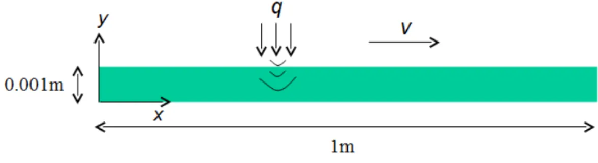
Fig. 2. Sketch of the geometry and process conditions. 3.2 2D numerical test

In this section we are considering the geometry and the process conditions sketched in Fig. 2. The calculation mesh consists of 1000 nodes in the length, 100 nodes in the thickness and 1000 time steps. We consider the previous gaus-sian flux with again A = 1, v = 0.1 and l = 0.05. The material thermal prop-erties are ρ = 1000 kg· m−3, Cp = 1000 J· kg−1· K−1, λx = 5 W· K−1· m−1

and λy = 0.5 W· K−1· m−1, which allows computing the diffusivity values:

kx = _ρλ_·Cx_p and ky = _ρλ_·Cy_p.

Figure 3 depicts the most relevant functions involved in the separated repre-sentation of the temperature field Xi(x), Yi(y) and Ti(t), i = 1,· · · , 4. The

reconstructed solution obtained from these functions is depicted in Fig. 4 at different times that correspond to different positions of the thermal source moving on the surface y = H = 0.001.

3.3 3D numerical test

The procedure detailed above can be easily extended to 3D geometries. For that purpose it suffices to consider the space-time separated representation of

0 2 4 6 8 10 −0.25 −0.2 −0.15 −0.1 −0.05 0 0.05 0.1 0.15 0.2 0.25 t (s) T i 0 0.2 0.4 0.6 0.8 1 −0.25 −0.2 −0.15 −0.1 −0.05 0 0.05 0.1 0.15 0.2 0.25 x (m) X i −5 0 5 x 10−4 0 0.2 0.4 0.6 0.8 1 1.2 1.4 1.6 1.8 2x 10 4 y (m) Y i

Fig. 3. Most significant functions involved in the separated representation of the temperature field.

Fig. 4. Reconstructed thermal field at different times obtained from the separated representation whose functions are depicted in Fig. 3.

the temperature field in a hexahedral tape

u(x, y, z, t)≈

N

∑

i=1

Xi(x)· Yi(y)· Zi(z)· Ti(t) (36)

that is constructed by a simple extension of the iteration procedure described previously.

To prove the feasibility of such extension to higher dimensional models we consider the geometry addressed in the previous 2D example extruded in the

z-direction with a depth of 0.2m. Thus, (x, y, z) ∈ Ω, Ω = Ωx × Ωy × Ωz,

with Ωx = (0, L = 1m), Ωy = (0, H = 0.001m) and Ωz = (0, D = 0.2m). We

consider that the thermal flux does not vary in the z-direction such that the expression previously considered remains valid:

q(x, z, t) = A· 1 l√2π. exp ( −(x− vt)2 2l2 ) (37)

whose separated representation reads again: q(x, z, t)≈ i=Q_∑ i=1 Fi(x)· Hi(z)· Gi(t) (38) with Hi(z) = 1,∀i.

We consider 1000, 100 and 1000 nodes for discretizing Ωx, Ωy and Ωz

respec-tively. Due to the uniformity of the solution in the z-direction, a very coarse discretization in that direction suffices, but we prefer to consider a mesh fine enough to highlight the capabilities of PGD and the interest of the coordinates separation. We consider as previously 1000 time steps. Of course, if one wants to solve the same problem using a standard mesh based discretization tech-nique, the resulting model contains 1000× 100 × 1000, i.e. 108 _{nodes (degrees}

of freedom), and then, in the general case of non-linear material models one must solve 1000 times a system of size 108_{, that is practically intractable.}

By using the PGD this solution is computed in around one minute by using Matlab on a standard laptop. Instead of solving 1000 times, a systems of size 108 _{we must solve of the order of N 1D problems of size 1000 (leading to}

tridiagonal matrices) for computing functions Xi(x) (i = 1,· · · , N), of the

order of N 1D problems of size 100 for computing Yi(y), of the order of N 1D

problems of size 1000 for calculating Zi(z) and of the order of N 1D initial value

problems for computing Ti(t). These calculation can be performed incredibly

fast even in the non-linear case [4].

Figure 5 depicts the reconstructed solution, where for visualization purposes we represented the temperature field (using a color map) on different sections along the tap thickness, without respecting the geometrical scale.

Fig. 5. Reconstructed temperature field at t = 5s.

4 Conclusion

In this paper we addressed the issue of fully space-time separated represen-tations of thermal models defined in tape-type domains. These degenerate geometries are more and more considered in composite forming processes jus-tifying the interest for fast and accurate simulations of processes, especially in the case of tricky process conditions involving moving thermal sources applied on the domain boundary.

We proposed a fully separated representation that transforms a three dimen-sional transient problem into a sequence of 4 one dimendimen-sional ones. The com-puting time savings can be simply spectacular, allowing the solution of models never solved until now due to the extremely large number of degrees of free-dom.

The use of the PGD opens a number of unimaginable possibilities, some of them are being explored, others are waiting for deeper analysis.

References

[1] A. Ammar, B. Mokdad, F. Chinesta, R. Keunings. A new family of solvers for some classes of multidimensional partial differential equations encountered in kinetic theory modeling of complex fluids. Journal of Non-Newtonian Fluid Mechanics, 139, 153-176, 2006.

[2] A. Ammar, D. Ryckelynck, F. Chinesta, R. Keunings, On the reduction of kinetic theory models related to finitely extensible dumbbells, J. Non-Newtonian Fluid Mech., 134, 136-147, 2006.

[3] A. Ammar, B. Mokdad, F. Chinesta, R. Keunings. A new family of solvers for some classes of multidimensional partial differential equations encountered in kinetic theory modeling of complex fluids. Part II: Transient simulation using space-time separated representation. Journal of Non-Newtonian Fluid Mechanics, 144, 98-121, 2007.

[4] A. Ammar, M. Normandin, F. Daim, D. Gonzalez, E. Cueto, F. Chinesta. Non-incremental strategies based on separated representations: Applications in computational rheology. Communications in Mathematical Sciences, 8/3, 671-695, 2010.

[5] R.A. Bialecki, A.J. Kassab, A. Fic, Proper orthogonal decomposition and modal analysis for acceleration of transient FEM thermal analysis, Int. J. Numer. Meth. Engrg., 62, 774-797, 2005.

[6] J. Burkardt, M. Gunzburger, H-Ch. Lee, POD and CVT-based reduced-order modeling of Navier-Stokes flows, Comput. Methods Appl. Mech. Engrg., 196, 337-355, 2006.

[7] F. Chinesta, A. Ammar, F. Lemarchand, P. Beauchene, F. Boust. Alleviating mesh constraints: Model reduction, parallel time integration and high resolution

homogenization. Computer Methods in Applied Mechanics and Engineering, 197/5, 400-413, 2008.

[8] F. Chinesta, A. Ammar, E. Cueto. Recent advances and new challenges in the use of the Proper Generalized Decomposition for solving multidimensional models. Archives of Computational Methods in Engineering, 17/4, 327-350, 2010.

[9] F. Chinesta, A. Ammar, A. Leygue, R. Keunings. An overview of the Proper Generalized Decomposition with applications in computational rheology. Journal of Non Newtonian Fluid Mechanics, 166, 578-592, 2011.

[10] Ch. Ghnatios, F. Chinesta, E. Cueto, A. Leygue, P. Breitkopf, P. Villon. Methodological approach to efficient modeling and optimization of thermal processes taking place in a die: Application to pultrusion. Composites Part A, .42, 11691178, 2011.

[11] D. Gonzalez, A. Ammar, F. Chinesta, E. Cueto. Advances in the use of separated representations. International Journal for Numerical Methods in Engineering, 81/5, 637-659, 2010.

[12] M.D. Gunzburger, J.S. Peterson, J.N. Shadid, Reduced-order modeling of time-dependent PDEs with multiple parameters in the boundary data. Comput. Methods Appl. Mech. Engrg., 196, 1030-1047, 2007.

[13] P. Ladeveze, Nonlinear computational structural mechanics, Springer, NY, 1999.

[14] P. Ladeveze, J.-C. Passieux, D. N´eron. The LATIN multiscale computational method and the proper generalized decomposition. Computer Methods In Applied Mechanics and Engineering, 199/21-22, 1287-1296, 2010.

[15] Y. Maday, E.M. Ronquist, The reduced basis element method: application to a thermal fin problem, SIAM J. Sci. Comput., 26/1, 240-258, 2004.

[16] D. N´eron, P. Ladev`eze. Proper generalized decomposition for multiscale and multiphysics problems. Archives of Computational Methods In Engineering, 17/4, 351-372, 2010.

[17] S. Niroomandi, I. Alfaro, E. Cueto, F. Chinesta. Real-time deformable models of non-linear tissues by model reduction techniques. Computer Methods and Programs in Biomedicine, 91, 223-231, 2008.

[18] S. Niroomandi, I. Alfaro, E. Cueto, F. Chinesta. Order Reduction for hyperelastic materials. International Journal for Numerical Methods in Engineering, 81/9, 1180-1206, 2010.

[19] H.M. Park, D.H. Cho, The use of the Karhunen-Love decomposition for the modelling of distributed parameter systems, Chem. Engineer. Science, 51, 81-98, 1996.

[20] E. Pruliere, F. Chinesta, A. Ammar. On the deterministic solution of parametric models by using the Proper Generalized Decomposition. Mathematics and Computers in Simulation, 81, 791-810, 2010.

[21] D. Ryckelynck, A priori hyper-reduction method: an adaptive approach, Journal of Computational Physics, 202, 346-366, 2005.

[22] D. Ryckelynck, L. Hermanns, F. Chinesta, E. Alarcon, An efficient ”a priori” model reduction for boundary element models, Engineering Analysis with Boundary Elements, 29, 796-801, 2005.

[23] D. Ryckelynck, F. Chinesta, E. Cueto, A. Ammar, On the a priori model reduction: overview and recent developments, Archives of Computational Methods in Engineering, 13/1, 91-128, 2006.