HAL Id: tel-01220524
https://pastel.archives-ouvertes.fr/tel-01220524
Submitted on 26 Oct 2015
HAL is a multi-disciplinary open access
archive for the deposit and dissemination of
sci-entific research documents, whether they are
pub-lished or not. The documents may come from
teaching and research institutions in France or
abroad, or from public or private research centers.
L’archive ouverte pluridisciplinaire HAL, est
destinée au dépôt et à la diffusion de documents
scientifiques de niveau recherche, publiés ou non,
émanant des établissements d’enseignement et de
recherche français ou étrangers, des laboratoires
publics ou privés.
variation for online application in automotive cold
rolling process
Quang Tien Ngo
To cite this version:
Quang Tien Ngo. Thermo-elasto-plastic uncoupling model of width variation for online application in
automotive cold rolling process. Mechanics of materials [physics.class-ph]. Université Paris-Est, 2015.
English. �NNT : 2015PESC1063�. �tel-01220524�
———————————
Thesis
for obtention of Doctor of Science of Paris-Est University
Thermo-elasto-plastic uncoupling model of width variation
for online application in automotive cold rolling process
presented on 30th March 2015 by
NGO Quang Tien
to the jury composed of
Pierre MONTMITONNET
Professor, CNRS Research Director
President
Cemef - MINES ParisTech
Habibou MAITOURNAM
Professor, Mechanical Unit Director
Rapporteur
ENSTA ParisTech
Ahmed BENALLAL
Professor, CNRS Research Director
Rapporteur
LMT - ENS Cachan
Nicolas LEGRAND
PhD, Research & Development Engineer
Examiner
ArcelorMittal USA
Alain EHRLACHER
Professor, GMM department Director
Director
In order to save material yields in cold rolling process, the thesis aims at developing a predictive width variation model accurate and fast enough to be used online. Many efforts began in the 1960s in developing empirical formula. Afterward, the Upper Bound Method (UBM ) became more common. [Oh 1975]’s model with 3D "simple" velocity field estimates well the width variation for finishing mill rolling conditions. [Komori 2002] proposed a combination of fundamental ones to obtain a computer program depending minimally on the assumed velocity fields. However, only two fundamental fields were introduced and formed a subset of the "simple" family. [Serek 2008] studied a quadratic velocity family that includes the "simple" one and leads to better results with a higher computing time.
Focusing on UBM , the first result of the thesis is a 2D model with an oscillating velocity field family. The model results to an optimum velocity that oscillates spatially throughout the roll-bite. The optimum power and the velocity field are closer to Lam3-Tec3 results than the "simple" one. For 3D modelling, we chose the 3D "simple"
UBM and carried a comparison to the experiments performed at ArcelorMittal using narrow strips [Legrand 2006].
A very good agreement is obtained. Further, a new UBM model is developed for a crowned strip with cylindrical work-rolls. It shows that the width variation decreases as a function of the strip crown and the results match well those of Lam3-Tec3 . However, the UBM considers only a rigid-plastic behaviour while in large strip rolling, the elastic and thermal deformations have important impacts on the plastic one. There exist some models considering these phenomena [Counhaye 2000, Legrand 2006] but they are all time-consuming. Thus, the idea is to decompose the plastic width variation into three terms: total, elastic and thermal width variations through the plastic zone that are determined by three new models. The simplified roll-bite entry & exit models allow estimating the elastic and plastic width variations before and after the roll-bite. They give equally the longitudinal stresses defining the boundary conditions for the roll-bite model which is indeed the 3D "simple" UBM approximating the total width variation term. Moreover, with the plastic deformation and friction dissipation powers given by the same model, the thermal width variation term is also obtained. The width variation model, called UBM -Slab combined is very fast (0.05s) and predicts accurately the width variation in comparison with Lam3-Tec3 (<6%).
Résumé
Dans le but d’optimiser la mise aux milles au laminage à froid, la thèse consiste à développer un modèle prédictif de variation de largeur à la fois précis et rapide pour être utilisable en temps réel. Des nombreux d’efforts ont commencé en 1960s en développant des formules empiriques permettant d’estimer la variation de largeur au laminage. Mais par la suite, la Méthode des Bornes Supérieures (MBS) est devenue la plus connue grâce à sa simplicité et efficacité. A ce sujet, il sera un manque de ne pas parler de [Oh 1975] avec le champ de vitesse 3D "simple", [Komori 2002] avec une méthode de combinaison des champs de vitesse et [Serek 2008] avec le champ de vitesse quadratique.
En approfondissant la méthode, le premier résultat obtenu dans la thèse est un modèle 2D (MBS) avec des champs de vitesse oscillante. Ce champ de vitesse particulier a abouti à des résultats (puissance, vitesse...) plus proches de ceux de Lam3-Tec3 que d’autres champs de vitesse étudiés dans la litérature. Pour une modélisation de variation de largeur, j’ai choisi la MBS avec la vitesse 3D "simple" et obtenu un très bon accord avec les expériences réalisées sur des produits étroits à ArcelorMittal [Legrand 2006]. En outre, un nouveau modèle MBS est développé pour une bande bombée et des cylindres droits. Les résultats montrent que la variation de largeur diminue avec la bombée de la bande et correspondent bien à ceux de Lam3-Tec3 . Cependant, la MBS admet un comportement rigide-plastique tandis qu’au laminage des bandes larges les déformations élastique et thermique ont des impacts importants sur la déformation plastique. Afin d’obtenir un modèle rapide, l’idée a été de décomposer la variation de largeur plastique en trois termes: les variations de largeur totales, élastique et thermique et les déterminer par trois nouveaux modèles simplifiés. Les deux premiers permettent d’estimer les variations de largeur élastique et plastique en amont et en aval de l’emprise. Ils donnent aussi les conditions aux limites au modèle d’emprise qui est en effet la MBS avec le champ de vitesse 3D "simple" permettant d’estimer la variation de la largeur totale. En outre, avec les puissances de déformation et de dissipation plastique de frottement données par le même modèle, la variation de largeur thermique est également obtenue. Le modèle de variation de largeur est donc appelée UBM-Slab combiné, très rapide (0,05 s) et prédit avec précision la largeur de variation par rapport à Lam3-Tec3 (<6%).
I would like to acknowledge everyone who has assisted me throughout my doctoral studies over the years.
Firstly, I would like to give special thanks to my thesis director, professor Alain EHRLACHER (Navier laboratory - ENPC, Paris-Tech) who accepted me to perform this thesis in a particular financial condition. Then, he always directed and advised me with excellently creative ideas allowing me to advance on the topic. In addition, I am extremely grateful to him for his the encouragements at numerous difficult moments during the thesis. Without such supports I could have never completed the thesis successfully as it is.
A sincere thank to my industrial advisor Nicolas LEGRAND (ArcelorMittal Global Research & Development) for his guidance and orientation that inspired my works and developments. He is also the person who initiated, con-structed the subject and supported me to perform this thesis.
I would like to appreciate Pierre-Stéphane MANGA, manager of Cold plant service and Marie-Christine REG-NIER, manager of Downstream Processes department who always made the best conditions for me to work on the thesis. My sincere thanks to my previous managers Akli ELIAS and Daniel LAUNET as well as to ArcelorMittal direction for their agreement and support to this project. Thanks to Camille ROUBIN, Maxime LAUGIER and Eliette MATHEY and all my other colleagues for their prestigeful technical exchanges which strongly enriched me about rolling process culture.
I highly appreciated professor Ahmed BENALLAL at LMT - ENS Cachan, CNRS Research Director and pro-fessor Habibou MAITOURNAM, Mechanical Unit Director at ENSTA for accepting to be my thesis rapporteurs as well as for their careful lecture and very worthy recommendations. I would like to acknowledge professor Pierre MONTMITONNET, CNRS Research Director, Cemef - MINES ParisTech for agreeing to be the committee president.
Very special thanks to my parents, my sisters and my brother as well as all my friends for their inducement and expectation that became my great motivation to become doctor.
I express, finally my all appreciation to my wife and my two daughters for supporting all my endeavours. They are my daily inexpiable sources of motivation.
Objective
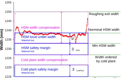
Cold rolling of flat products is nowadays one of the main forming processes in metallurgical industry. The process geometry seems simple but its control requires the understanding of intricate thermo-mechanical aspects. In cold rolling process, due to the reduction in thickness the strip width is also changed. It is observed that in most of the cases the strip width decreases. And this width variation an be up to more than 10mm while it is not predicted in the production plants. By consequence, the plants produce usually an over-width in order to ensure the customer requirement and this over-width leads to an important over-cost of the production.
One solution to reduce the over-width consists in using a predictive model of width variation for each process in general and for cold rolling in particular. Such a model enables to determine the necessary width at the entry of cold rolling process to produce the required width. However, the over-width is not eliminated. It is still necessary to take an over-width due to the uncertainty of the model. Therefore, the more accurate the model the lower the unavoidable over-width. That means, even with a predictive model the production is set up to get an over-width in most of the cases and an under-width otherwise. In addition, products provided by hot rolling mill have usually different width in comparison with what the cold rolling mill requires and it varies all along the product. It is, thus also benefiting to adjust online the width in cold rolling process by varying some rolling parameters. For these reasons, the thesis aims at developing a predictive width variation model for cold rolling process which is accurate and fast enough to be used in real-time production.
Bibliographic reviews
2D simplified models in literature A
In the beginning of the 20th century when the computer science notion had never ever existed, there were many efforts to develop analytical rolling models. The two famous families of models are slab method based on the well-known equilibrium equations pioneered by [113] in 1925 and Orowan’s theory [86] considering the inhomogeneity of stresses across strip thickness. Around the 1950s, simplified methods were introduced in order to take into account the strip elastic deformation [16,17] before that Cosse [27] proposed the first complete elasto-plastic model in 1968.
In parallel with the developments of models for strip deformation, there exist equally divers models for the work-roll deformation. The very first one, Hitchcock’s model [46] considers that the deformed work-roll remains circular with a higher diameter. This model is still used today by a large number of models for industrial rolling preset. It is modified in 1952 by [17] to take into account influence of the elastic deformation areas. Later, in 1960 [52] proposed to determine the deformation of each point on the surface of the roll by a sum of influence function of each finite element with a specific pressure distribution. The method approaches accurately the work-roll profile. Fleck and Johnson [36] investigated on thin strip rolling and were the firsts who consider the existence of elastic deformation areas inside the roll-bite (the strip deformation is elastic and plastic alternatively) as well as the existence of a neutral zone instead of a neutral point previously. This model is a significant progress to approach rolling process of very thin strip such as packaging products.
With variation models in literature A
Concerning existing models of width variation in rolling process, important effort began in the area of the 1960s in developing empirical formula to predict the width variation - [115,104,43,14]. Afterward, with the appearance of computer science there existed many analyses using FEM for flat and shape rolling such as [77,78,54] where the shape and the spread are predicted and [76] where a complete thermo-mechanical solution could be found. In order to reduce the computing time certain authors, based on the Upper Bound Method (UBM ), developed numerical method for integration which is similar to FEM , [58,1]. The UBM became more and more common to approach the width variation problem thanks to its simplicity and rapidity. In addition, unlike the empirical models mentioned above, the
UBM is physical and fully predictive.
2D UBM models for rolling process A
As for UBM , that is an extremum principle for perfectly plastic solids formulated by [91] which states that among all kinematically admissible strain rate fields the actual one minimizes the potential power. This method is largely used to obtain approximate solution to forming processes problems. By nature, the UBM result depends strongly on the choice and the construction of velocity fields. In the literature, there exist two categories of velocity fields. The first one considers rigid bodies motions (called also slip lines) and the second one includes continuous velocity fields to model the plastic deformation zone. In 1973, Johnson and Mellor [51] analyzed strip rolling by the unitriangular velocity field based on the curvilinear triangle, opening a new avenue of approach for the UBM . In 1986, Avitzur and Pachla [10] introduced the concept of neighboring rigid body zones which were applicable to strip drawing, extrusion, forging, rolling, drawing, cutting processes. Camurri and Lavanchy [22] developed in 1984 a velocity fields with multitriangles slip lines. This model has been reanalyzed by Avitzur, Talbert and Gordon [12] by using the concept presented in [10]. With multitriangular velocity field, the meaning of the neutral region becomes evident. That is one of triangular regions that rotates with the same rotational velocity as the work-roll. This model allows improving the optimum power but the resolution of optimization problem becomes however much more complicated in comparison with the unitriangular one.
On the subject of continuous category, around 1963 Avitzur [5,6,7] proposed the "eccentric" velocity field. The author defined the arcs connecting any two symmetrical points on the opposing rolls. These arcs are eccentric and each one meets the roll surfaces at right angles. The velocity of each material point on an arc is on the direction of the its radius. With this velocity field, Avitzur obtained an analytical solution to the power optimization problem by assuming small angle approximation. In 2001, Dogruoglu [31] based on flow function concept, introduced a method for constructing kinematically admissible velocity field by pre-assuming the form of the flow lines. In one of his applications, the flow lines are chosen being "elliptical" and led to an optimum power that is smaller (better) than that obtained by the eccentric velocity field. Later, Bouharaoua and al [18] by assuming that a material cross section stays vertical all along the roll-bite (equivalent the slab method assumption), obtained a velocity field called "simple" one. In the present thesis, we demonstrate that this field and the elliptical one are exactly the same in the case of circular work-roll.
Rigid-plastic 3D UBM models for prediction of width variation A
In 1975, Oh & Kobayashi [83] are two of the pioneers who applied the UBM to 3D rolling process analysis. The authors supposed a 3D "simple" velocity field which is in the analogy of the 2D "simple" one. The longitudinal velocity is constant on an across section and the vertical and lateral velocities are linear in the thickness and width directions correspondingly. In 2002, K. Komori [59] proposed to represent the velocity field as a linear combination of predefined fundamental ones. With this new method of analysis, the structure of the computer program depends minimally on the assumed kinematically admissible velocity fields. Nevertheless, it is not so easy to propose fundamental velocity fields. In the article, only two fundamental fields are mentioned for demonstration. Moreover, in the present thesis, we brought out that Komori’s velocity field [59] is indeed included in the "simple" family. Later, Serek [99] proposed a method for constructing kinematically admissible velocity fields by means of Dual Stream Function (DSF). This DSF was introduced by [117] allowing to express the three velocity components as functions of two scalar fields and the incompressibility condition is satisfied. The rigid plastic boundary at the inlet zone is quadratic instead of a plane section by the "simple" velocity field. The results obtained from the analysis are compared with experimental results and a good agreement is found confirming the UBM efficiency to approach the width variation in rolling.
Achievements
2D UBM analysis and oscillation phenomenon of mechanical fields in rolling process A
As mentioned above, Dogruoglu’s method allows determining the velocity field based on the predefined stream lines. However, it is very difficult to imagine a very good and complete flow lines. For this reason, until today, except circular and elliptical flow lines, there does not exist any other imagined flow lines pattern to approach rolling process. In the chapter4 we presented a method for constructing kinematically admissible velocity fields based on the DSF method. Any kinematically admissible velocity field can be given as the sum of the "simple" (or elliptical) one and an additional term. By observing that the equations of kinematically admissible conditions of the additional term are closely similar to the wave propagation ones, we proposed a new family of "oscillating" velocity fields. Further, applying the UBM to this new velocity family results to an optimum velocity that oscillates spatially throughout the roll-bite with pseudo-period equal to the local strip thickness. The rolling power obtained with this oscillating velocity field is smaller than the one with the simple (elliptical) velocity field. The results of this model match very well those obtained by Lam3-Tec3 in terms of velocity field, plastic deformation zone and flow lines. As a result of the
UBM model as well as Lam3-Tec3 , the mechanical fields heterogeneity is non-linear, quasi-sinusoidal across the strip
thickness. Whilst this heterogeneity remains little investigated.
Rigid-plastic 3D UBM model for flat strip A
Applying the method proposed in the chapter4any 3D velocity field is also composed of 3D "simple" one and an additional term. The characteristics of this additional term are analyzed. Nevertheless, in order to keep a fast computing time of the power optimization resolution, we carried out the study of width variation using the 3D "simple" velocity field. The integrations are done using Gauss’s method allowing accelerating the computing time. A comparison with experiments has showed a very good coherence. These experiments have been performed in ArcelorMittal pilot mill with relatively narrow strips (we≃60−70mm).
In addition, with this 3D "simple" UBM model, an analysis has been realized and pointed out the effect of rolling parameters on the strip width spread. As results for a narrow strip, the width spread increases strongly with an increase in the reduction and falls down exponentially as a function of the strip entry width. It grows almost linearly as the roll radius increases and decreases with an increase in the entry or exit tensions. These results are coherent with existing works in the literature.
Rigid-plastic 3D UBM models for crown strip A
Some studies using a mixture of analytical and numerical methods [109,73,3,30,29] pointed out that for thin strip rolling, the spread is small. Nevertheless, these studies showed out that the exit thickness profile of the strip (closely linked to the strip flatness) can influence the strip lateral spread.
Interested in this phenomenon, a new UBM approach is developed for cold rolling of strip with initial thickness crown while the work-roll is considered rigid and perfectly cylindric. First, an analysis is proposed to study kinemat-ically admissible velocity fields in supposing some hypotheses. As the geometry of the strip is more complex than the case of flat strip rolling, the roll bite is divided into three areas in which the velocity field is different. The model shows that the width variation decreases with an increase in the strip initial crown. These results match very well those obtained with Lam3-Tec3 . Moreover, as can be noted, the strip crown increases the strip thickness reduction is higher at the strip center than at the edges that leads to a flatness defect called "center wave". Thus, the more the strip crown, the more "center wave" and the smaller the strip spread that can even be negative (necking).
UBM - Slab combined model to predict thermo-elasto-plastic width variation in industrial conditions A
As previously seen, the UBM model for flat and crowned strip in rolling process match well the experiments on pilot mill as well as Lam3-Tec3 . However, it is worth to highlight that the UBM assumes a rigid-plastic behavior of the strip that is justified for narrow strip rolling because the elastic width variation are negligible. On the opposite, in automotive industrial rolling condition the strip is large and the elastic width variation which is proportional to the strip width is no longer negligible. This elastic deformation is reversible but it has important impact on the plastic one. In addition, friction and plastic deformation powers heat up the strip. The material is, thus dilated in the width direction
but it can not because of the contact friction with the roll. That creates compression plastic deformation - called thermal contraction. After a bibliography review a new width variation model for online applications is developed taking into account the effects of elastic and thermal deformations in addition to the width variation of UBM for flat strip rolling mentioned above.
An analysis of Lam3-Tec3 simulations about the impact of elastic and thermal deformation leads to a conclusion that the elastic deformation as well as the thermal dilatation of the strip in the roll-bite create a plastic deformation of a same amplitude but with an opposite sign. By consequence, the plastic width variation can be decomposed by three terms: the total width variation in the roll-bite, the elastic and the thermal width variations between the first and last points of plastic deformation. In order to determine these three terms, we develop simplified models for the entry, exit and inside the roll-bite as follows.
Simplified models for the entry and exit of the roll-bite: By assuming a homogeneous stress in thickness as the slab method, new simplified models are developed and allow to approximate the solution of strip deformation before and after the roll-bite. In other words, the models give us the spring back width variation at the roll-bite exit and the compression width variation at the entry. They give equally an approach of longitudinal stress just before and after the roll-bite area defining the boundary conditions for the roll-bite model.
Simplified model for the roll-bite: Thanks to the understanding of the impact of elastic and thermal deformation, the total width variation in the roll-bite is estimated close to the rigid-plastic width variation. This term can be, thus determined by the rigid-plastic UBM with 3D "simple" velocity field developed in the previous chapter. The boundary conditions (longitudinal stress tensor) at the roll-bite entry and exit are given by the roll-bite entry and exit models instead of entry and exit tensions initially imposed. Moreover, as the plastic deformation and friction dissipation powers are also determined by this model, the increase of strip temperature and the thermal width variation term are therefore determined. The width variation model is hence completed. This simplified thermo-elasto-plastic width variation model is called the UBM-Slab combined model.
Fast computing time enables online applications: As the model for roll-bite entry is completely analytical and the exit one is quasi-analytical, the main computing time is related to the roll-bite model - the rigid-plastic UBM . Thanks to the analytical development of the powers computation the total computing time of the width variation model (in C++) is less than 0.05s (CPU: Intel Core I5-4200M, 250GHz) enabling online applications such as preset or dynamic control.
Good prediction width variation: A comparison between the UBM-Slab combined model and Lam3-Tec3 is performed and a very good agreement is observed. The total plastic width variations obtained with the two models are very closed (less than 6% for stands 1, 2 & 3 and about 10% for the last stand making very small reduction). Finally, the UBM-Slab combined model allows studying the influence of rolling parameters not only on the final width variation but also on each contributing terms (roll-bite width variation, elastic or thermal deformation contributions) for a deeper understanding. The results match really well the tendencies observed in industrial data presented by some studies existing in literature [64].
Nomenclature
Symbols Meaning
A
νr, ν Poisson’s coefficient of the roll and the strip Er, E Young modulus of the roll and the strip
he, hs Strip half thickness before and after the roll-bite δ=he−hs Absolute thickness reduction
r=1−hs
he Relative thickness reduction
hrelaxe , hrelaxs Strip half thickness before and after roll-bite if there is no stress in the strip h Strip half thickness function in the roll-bite
hrelaxe , hrelaxs Strip half width before and after roll-bite if there is no stress in the strip we, ws Strip half width before the roll-bite
w Strip half width function in roll-bite Se, Ss Strip cross section before the roll-bite S Strip cross section in the roll-bite xe, xs x-position of entry and exit section xn x-position of the neutral point
hn Strip half thickness at the neutral point
θ Position angle
θe, θn Position angle at roll-bite entry and at neutral point Ve, Vs Strip velocity before the roll-bite
Vc Peripheral velocity of the roll Fe, Fs Entry and exit tensions (N) Te, Ts Entry and exit average stress (Mpa) te, ts Entry and exit adimensional average stress R, Rde f Work-roll initial and deformed radii µ, m Coulomb and Tresca friction coefficients σ0, k= √σ03 Strip yield stress and shear yield stress
σn Contact normal pressure (positive value by convention) τ Contact shear stress - friction stress
Cvol Material volume flow rate
L Contact length
F Roll force by an unit of width (N/mm) f s Forward slip (%)
Tq Roll torque by an unit of width (N.mm/mm=N.m/m) ξ, u Vector of displacement and vector of velocity
σ Stress tensor
ǫ, ˙ǫ Strain and strain rate tensors Jf ric Power consumed by friction
Jde f Power consumed by plastic deformation
J˙ǫ Power consumed by plastic deformation in the continuous velocity zones
J∆u Power consumed in the surfaces of discontinuity of velocity
Jten Power of entry and exit tensions
J Total power
Γe, Γs Surface of velocity discontinuity at roll-bit entry and exit x, y, z 3 Direction coordinates : longitudinal, lateral and vertical
Abstract 0
Thanks i
Long abstract i
Nomenclature v
1 Width variation problematic in steel rolling 1
1.1 Introduction to steel . . . 2
1.2 Typical steel production route. . . 3
1.3 Width variation problematic in cold rolling process . . . 15
1.4 Thesis objective and approaches . . . 19
2 Rolling process modeling reviews 21 2.1 General description of rolling problem . . . 22
2.2 Typical tribological models . . . 28
2.3 Typical strip models. . . 31
2.4 Typical work-roll deformation models . . . 45
2.5 Discussions . . . 49
3 Upper Bound Method applied in rolling process 51 3.1 Principle of the UBM . . . 52
3.2 Velocity fields with rigid bodies motions . . . 56
3.3 2D continuous velocity fields . . . 62
3.4 Discussions . . . 69
4 Oscillation of mechanical fields in roll bite 71 4.1 Introduction . . . 72
4.2 Method for constructing velocity field . . . 72
4.3 An oscillating velocity field proposal. . . 76
4.4 UBM with the oscillating velocity field . . . 79
4.5 Comparison with Lam3-Tec3 and other UBM models . . . 86
5 Rigid-plastic UBM model for width spread 97
5.1 Statistical models for width spread . . . 98
5.2 3D rigid-plastic UBM for width variation analysis . . . 99
5.3 Chosen rigid-plastic model of width variation in rolling . . . 105
5.4 Conclusions and perspectives . . . 117
6 UBM for crowned strip rolling 123 6.1 Velocity field proposition . . . 124
6.2 Calculation of the powers . . . 129
6.3 Numerical resolution . . . 131
6.4 Comparison between UBM and Lam3-Tec3 . . . 132
6.5 Conclusion . . . 133
7 A thermal-elastic-plastic width model 135 7.1 Bibliographic review on width variation in industrial cold rolling . . . 136
7.2 Analytical thermal-elastic-plastic width variation model . . . 143
7.3 A simplified entry elasto-plastic compression model. . . 151
7.4 A simplified elastic spring back model - elastic slab method. . . 153
7.5 A simplified model for roll-bite. . . 158
7.6 Summary . . . 160
8 The UBM-Slab combined model validation 163 8.1 Simplified model algorithm and programming . . . 164
8.2 Validation by comparison with Lam3-Tec3 . . . 165
8.3 Validation by comparison with industrial observations. . . 168
8.4 Conclusions . . . 171
9 General conclusions and perspectives 175 9.1 Conclusions . . . 175
9.2 Perspectives . . . 176
Appendix
178
A Numerical Gauss-Legendre integration 179 A.1 Principle. . . 179A.2 Applications. . . 181
B Calculation of powers 183 B.1 Calculation of power of plastic deformationJ˙ǫfor the simple 2D velocity field . . . 183
C Experiment on narrow strips 189
C.1 Rolling parameters . . . 189
C.2 Lam3-Tec3 modeling . . . 190
Width variation problematic in steel rolling
The present chapter is an introduction to the subject of the thesis. In the first two sections the steel production route is presented briefly. That points out where hot and cold rolling processes are found, clarifies their roles and reason for existence. The third part presents the width variation problematic in the whole production route and the importance of predictive models for the setup of the strip width during its production. The material yield caused by over-width is the main issue for what a rapid and predictive model of width variation in cold rolling is developed. That is the goal of this study presented in the fourth section of the chapter together with the development methodology. In the last place, the fifth section demonstrates the structure of the thesis.
Contents
1.1 Introduction to steel . . . . 2
1.1.1 Steel applications. . . 2
1.1.2 Steel and metallurgy history . . . 2
1.2 Typical steel production route . . . . 3
1.2.1 Liquid steel . . . 3
1.2.2 Secondary metallurgy and casting . . . 7
1.2.3 Hot rolling plant . . . 8
1.2.4 Cold rolling plant. . . 10
1.3 Width variation problematic in cold rolling process . . . . 15
1.3.1 Industrial observation. . . 15
1.3.2 Width specification using prediction models. . . 15
1.3.3 Over-width material yield . . . 17
1.3.4 Two ways reducing material yield . . . 18
1.4 Thesis objective and approaches . . . . 19
1.4.1 Thesis objective - predictive model for cold rolling process. . . 19
1.1
Introduction to steel
1.1.1
Steel applications
Steel is one of the materials the most used over the world. Talking about steel induces thinking of strength, dura-bility, safety and cleanliness. That is why we can find steel anywhere in our daily life. The steel applications field can be classified into five main domains.
1. Automotive industry: Car white body is composed of thin, flat carbon steel. High strength steel and stainless steel are used for structure, reinforcement and safety parts. Wheel and suspension parts are also made by strength steel while engine is long product steel. We can also find steel in many other pieces of a car as: tyre reinforcement (steel cord), exhaust system and decoration (stainless, aluminized or chromium steel). More than a half of car weight is made from steel.
2. Packaging: food containers, drink cans, liquid and gas containers. These consumable products are made from steel partly because of the steel high recyclability. It is incredibly true that drink cans made from steel could be recycled infinite of times. For this application, we use mostly thin law carbon steel resisting to high pressure. High quality of surface is required because steel is coated (health safety) and painted.
3. Household appliances: Many kitchen objects as oven, refrigerator, washing machine, sink... are made from painted low carbon steel, enameling steel and stainless steel. And thanks to its health safety, cleanliness and very high strength, stainless steel is most used for cooking utensils and cutlery.
4. Construction and mechanical industry: Thanks to very interesting ratio strength/weight and high durability, steel always keep its place in construction market among numerous number of materials. Many bridges, offshore platforms, boats and sheet pilings are made from heavy steel plates, high strength beam and wires. All rails are high carbon long steel product. Steel is also used to produce: tubes, pipes, tanks for petrol, chemical and food industries as well as transportation or specific products like pressure vessels and springs...
5. Building: There are more and more building with steel structure using steel beam (long product), flat panels, roofs. Different from other material stainless steel or painted and coated steel are used for decoration.
In the present thesis, we are interested in rolling process of flat carbon steel for automotive and packaging applica-tions. Thus, after a brief history of metallurgy, the production route of these kinds of steels, considered representative for general steel production, will be presented.
1.1.2
Steel and metallurgy history
The discovery of steel: By the 11th century BC it has been discovered that iron can be much improved. If it is reheated in a furnace with charcoal (containing carbon), some of the carbon is transferred to the iron. This process hardens the metal. In addition this effect is considerably greater if the hot metal is rapidly reduced in temperature, usually achieved by quenching it in water. The new material is steel. It can be worked just like softer iron, and it will keep a finer edge, capable of being honed to sharpness. Gradually, from the 11th century onwards, steel replaces bronze weapons in the Middle East, birthplace of the Iron Age.
The first cast iron: Thus far in the story iron has been heated and hammered, but never melted. Its melting point (1528°C) is too high for primitive furnaces, which can reach about 1300°C and are adequate for copper (melting at 1083°C). This limitation is overcome when the Chinese develop a furnace hot enough to melt iron, enabling them to produce the world’s first cast iron - an event traditionally dated in the Chinese histories to 513 BC. In this they are a thousand and more years ahead of the western world. The first iron foundry in England, for example, dates only from AD 1161. By that time the Chinese have already pioneered the structural use of cast iron, using it sometimes for the pillars of full-size pagodas.
Ironmasters of Coalbrookdale: Until the early 18th century the working of iron has been restricted by a practical consideration. The melting of iron requires large quantities of charcoal, with the result that ironworks are usually sited inaccessibly in the middle of forests. And charcoal is expensive. In 1709 Abraham Darby, an ironmaster with a furnace at Coalbrookdale on the river Severn, discovers that coke can be used instead of charcoal for the smelting of pig iron. This Severn region becomes Britain’s centre of iron production in the early stages of the Industrial Revolution. Its pre-eminence is seen in the Darby family’s own construction of the first iron bridge, and in the achievements of John Wilkinson.
Ironbridge 1779: In the space of a few months in 1779 the world’s first iron bridge, with a single span of over 100 feet, is erected for Abraham Darby (the 3rd of that name) over the Severn just downstream from Coalbrookdale. Work has gone on for some time in building the foundations and casting the huge curving ribs. But in this new technology little time need be spent in assembling the parts - which amount, it is proudly announced, to 378 tons of metal.
Puddling and rolling 1783-1784: In successive years Henry Cort, an ironmaster with a mill near Fareham in Hampshire, patents two processes of lasting significance in the story of metallurgy. One is the technique which becomes known as puddling. Cort’s innovation is a furnace which shakes the molten iron so that air mingles with it. Oxygen combines with carbon in the metallic compound, leaving almost pure iron. Unlike the brittle pig iron (or cast iron), this purer metal is malleable. Capable of being hammered and shaped, it is a much more useful metal in industrial processes than cast iron.
In the previous year Cort has also patented a machine for drawing out red-hot lumps of purefied metal between grooved rollers, turning them into manageable bars without the laborious process of hammering. His device is the origin of the rolling mills which subsequently become the standard factories of the steel industry.
Steel growth since the last century: The world-wide steel industry has tremendous growth during the 20th century, from an annual production of 20 million tons of steel in 1900 to more than 1.2 milliard tons nowadays. The most important growth rate has been performed in the 50s and 60s after the Second World War when the reconstruction as well as the economy and military concurrence in many countries required more and more steel. Another fast growth period is since 2000 when emerging countries as China, India... realize incredible economic growth. During this period the steel technology has been developed with a drastic rate as the evolution of sciences, engineering technologies and computer science. It is uncountable the number of scientific articles, books, thesis as well as numerous number of patents about the steel compositions and production processes.
1.2
Typical steel production route
1.2.1
Liquid steel
There are two ways to produce liquid steel, a classic way called "primary steel route" using iron ore and the other using steel scrap called "recycling route". This section has objective to introduce typical processes of steel production, their roles and particularities explaining their existence. The physical or chemical principle of certain processes are only shortly and roughly explained but not detailed.
1.2.1.a Primary route
Coke oven and sinter plant A
In a classic production route, raw iron ore follows first a sintering process to be purer. Today, after sintering the average iron ore charge varies from 70% up to 90%.
About coke, most of coke is man-made and obtained by pyrolysis of coal in regrouped furnaces in absence of air. This process, realized at about 1000°C, is called coke-making providing coke with high carbon content and few impurities. The coke is essential fuel for blast furnace thanks to its solidity, able to support charge and porosity allowing the transfer of gas and liquid through.
Blast furnace (BF) - Pig iron A
BF operates on the principle of chemical reduction whereby carbon monoxide, having a stronger affinity for the oxygen in iron ore than iron does, reduces the iron to its elemental form. Chemical reactions, control of temperature and the circulation of materials in the furnace are in fact complicated. Avoiding details of what happens, a very short description can be given as follows.
The main chemical reaction producing the molten iron, that might be indeed divided into multiple steps, is:
Fe2O3+3CO=2Fe+3CO2. (1.1)
The iron ore and coke are supplied through the top of furnace in successively forming alternative layers while the gas is flowed into furnace at the bottom (see Figure1.1). Going up, the gas is efficiently in contact with solids all along the furnace height. As output, the pig iron obtained and extracted at the bottom of the furnace contains generallyFe (93-95%),C (3-5%), Si (0.2-0.8%), Mn (0.2-2%) and also Al, S, P...
Ga s 1 5 0 0 m3 CO2 0 .7 t Coke 0 .3 t I ron ore s 1 .6 t 1 5 0 0 m3 Ore Coke Cohesive I nje c t ions 0 2 t Air 1 0 0 0 m3 zone H ot m e t a l Sla g 0 .2 t 1 0 0 0 m H ot m e t a l 1 t Sla g 0 .3 t
Figure 1.1: Blast furnace scheme and an approximated balance to obtain 1 ton of pig iron.
Limestone (CaCO3is provided into the top side in order to remove some impurities contained in iron ore notably
silicaSi. At the middle of the furnace, limestone is decomposed by reaction with CO2 and then the calcium oxide
obtained reacts with various acidic impurities (silica for example), to form a fayalitic calcium silicate. CaCO3→CaO+CO2
SiO2+CaO→CaSiO3
(1.2)
Slag is the liquid mainly composed of remaining of limestone decomposition and impurities of ironCaO, SiO2,Al2O3
andMgO as well as silicates of calcium (CaSiO3)of other metals ... The liquid slag floats on top of the liquid iron
since it is less dense and is removed continuously from the furnace bottom. At the furnace top side, the monoxide and dioxide of carbon are evacuated in the waste gas. Figure1.1gives approximated quantity of main inputs and outputs corresponding to a ton of hot metal (pig iron).
Basic oxygen furnace (BOF) - converter A
BF pig iron, containing 3-5%C, can be used to make cast iron but more often refined further to make steel (much lessC content. Liquid steel needs to contain lower contents of C, Mn, Si. Table1.1shows an example of composition of input pig iron and desired composition of liquid steel.
T C Mn Si P S O
°C % % % % % %
Liquid pig iron 1370 4.70 0.23 0.26 0.08 0.02 0.00
Liquid steel 1650 0.05 0.10 0.00 0.02 0.02 0.05
Table 1.1: Example of composition of pig iron supplied to BOF and liquid steel obtained.
Figure 1.2: Schema of BOF principle components. BOF allows refiningC content of pig iron at high temperature using oxygen.
Figure 1.3: Ellingham diagram: dependence of affinity for oxygen of different elements. Carbon affinity for oxy-gen increases with an increase in temperature while that of metals decreases.
To do that, the molten pig iron is poured into a Basic Oxygen Furnace (BOF) where most of the remaining carbon will be removed. In a BOF, pure oxygen is blown through a long tube, or lance inserted into the furnace top side. Sometimes, for higher stirring (to get lowerC content), oxygen is blown from the bottom side (see Figure1.2).
As can be seen in Figure1.3that the affinity for oxygen ofC at high temperature is much higher than that of Fe. Because other elements present in pig iron asAl, Mn, Si, Cr have also higher affinity for oxygen than Fe, they are equally almost removed from liquid pig iron by combining with oxygen to form oxide and stay in slag floating on the steel liquid such as:
2C+O2=2CO
Si+O2= (SiO2)
Mn+O2= (MnO2).
SinceS and P have similar affinity for oxygen as Fe (see Figure 1.3) they are more difficult to be removed. The solution is to add limestone to supplyCaO born after decomposition of CaCO3(see equation1.2). The basic reaction
to eliminateP is:
2P+5O+n(CaO) = (nCaO−P2O5) (1.3)
a stable oxide in slag. And the desulphurization is based two reactions S+ (CaO) = (CaS) +O S+2O=SO2.
1.2.1.b Recycling route
For a recycling route, the mail raw material is no longer iron ore (oxide ofFe) but steel scrap with various com-positions. Reducing oxides ofFe in BF and reducing C (and other impurities) in BOF are no longer necessary. Thus, instead of BF and BOF, Electric Arc Furnace (EAF) is used to melt scrap and produce directly liquid steel.
The cost of an EAF is about 8M C(Alternating Current - AC EAF) or 23M C(Direct Current - DC EAF) much lower than that required to build a BF (about 300M C). With lower productivity (about 0.7Mt per year), EAF is suitable for mini-mills. Invented in 1900, it had been used mainly for long products (bars, rods and small profiles) production. Today, EAF is also used to make flat carbon (thin slab casting) or heavy section products. Typically, better grades of steel products come from virgin iron ore and are rolled a great deal to fully develop internal quality and grain structure. In the market for midquality steels, the integrated can offer perhaps more than enough quality but often at too high cost. The mini-mills, in contrast, may have the right cost structure but not necessarily the right quality. By choosing suitable production route, companies can achieve a better pairing of cost and quality.
Figure 1.4: Illustrating the Electric Arc Furnace which uses scrap steel to produce pure steel.
Raw materials and elaboration A
For the production of steel in a EAF, the following principal raw materials are used as feedstock: • Recycled steel scrap
• Hot metal • Pig iron • Reduced iron
In general, three first materials (scrap, hot metal, pig iron) are charged into EAF before the actual elaboration starts and the reduced iron is continuously fed into the vessel during elaboration to adjust the target composition.
Heating A
The EAF principle is to heat material by electric arc through the metal between a graphite electrode inside and another at the bottom of the furnace thanks to a high voltage of about 1300V ((see Figure1.4). The heating can be divided into two steps: meltdown and super-hearing. During the first phase, the electrode starts from the top of the scrap charge, goes down close to the bottom to melt little quantify of scrap and form small metal bath. The electric
energy continues to melt scrap until obtaining flat bath (end of meltdown). After this meltdown phase, there remains some unmelted scrap, the superheating (refining) consists in melt them by moving the electrode inside the furnace and use lower level of power.
Almost all materials charged into the furnace can be oxidized and hence release some energy. Iron and tramp elements when oxidized are transferred from the steel bath to the slag while carbon containing elements are converted to furnace off-gas. Chemical energy is also entered using external divides as natural gas burners to assist meltdown avoiding cold spots in the vessel and oxygen & carbon lances providing oxygen for oxidation and post combustion.
Metallurgical results obtained at the EAF A
The remaining tramp elements (Cu, Sn, Ni, Mo, Sb...) in liquid steel depends on the scrap composition (scrap yard) while carbon and phosphorus content is result of the process (oxygen injection). Table1.2gives a rough idea about the composition of liquid steel obtained by EAF.
Process Scrap charge Cu Sn S P N C
ppm ppm ppm ppm ppm ppm EAF Low quality 250 50 50 40 70-90 40-50 Standard quality 150 20 30 15 70-90 High quality 50 10 10-20 <10 70-90 Scrap + few iron <50 <10 10-20 <10 40-50
BOF Pig iron 20 <5 10-20 <10 <20 10-40 Table 1.2: Comparison of chemical composition of liquid steel obtained by EAF and BOF
1.2.2
Secondary metallurgy and casting
Secondary metallurgy A
After BOF or EAF, the liquid steel enters into the refining process called secondary metallurgy which has primary objective to finely adjust chemical composition of steel in controlling impurities and metallic inclusions. This sec-ondary steelmaking process is most commonly performed in ladles. The necessary alloying elements are added while the impurities are removed by deoxidation (Al, Si), metal/slag reaction and vacuum degassing. Tight control of ladle metallurgy is associated with producing high grades of steel in which the tolerances in chemistry and consistency are narrow.
The second objective of the process is to prepare the right temperature of liquid steel just before casting process typically about 20°C more than liquidus temperature. A too low temperature may cause risk of solidification in the ladle or tundish while a too high temperature would make uncomplete solidification producing break at the casting machine exit. The ladles are commonly equipped of small electric arc furnace that is used to regulate the liquid steel temperature, for instance to re-heat the liquid steel when the casting process is delayed.
Continuous casting A
Figure1.5shows standard components of a casting machine. The ladles containing liquid steel are charged on the top side of the machine (feeding zone) where a rotating system allows replacing a full ladle into the position of an empty "in casting" ladle at the end of each casting "sequence". The liquid steel flows from the ladle to a tundish where the steel is well protected thermally and chemically. The tundish aims at feeding several strands in liquid steel and is a buffer tank during ladle change. It enables to control and regulate the steel flow rate in molds.
After the feeding zone, the steel comes in the molds, head zone, where heat is extracted to form primary solidified shell and give suitable geometry. Out of mold, the steel comes into solidification zone with many rolls guiding the change of direction from vertical to horizontal. The steel is solidified completely with position of the end of solidifica-tion depends on steel grade and process parameters. After an oxy-cutting process, solid steel slabs are produced with a dimension required by hot rolling plant.
Figure 1.5: Continuous casting machine: 1-Ladle, 2-Tundish, 3-Mold, 4-Plasma torch, 5-Stopper, 6-Straight zone.
After casting machine, automotive and packaging product slabs have generally a dimension of about 5-15m (Length) x 800-2000mm (Width) x 220-260mm (Thickness) weighting from 20 to 35tons. In a same casting sequence, the slabs have same width and thickness. It is necessary to note that casting machine only produces certain values of width, for example 800mm, 1200mm, 1600mm and 2000mm but not any desired one.
1.2.3
Hot rolling plant
The objective of a Hot Strip Mill (HSM) is to reduce the product thickness and width while controlling the product surface quality and mechanical properties. Different installations of a HSM can be described as follows (see Figure1.6). Hot rolling is also called hot metalworking process which consists in deforming product above the phase transformation temperature of the material because:
• at austenite phase, material is much softer
• at higher temperature, the grains deform during rolling, they recrystallize, which maintains an equiaxed mi-crostructure and homogenous grains size.
• the phase transformation needs to be precisely performed to get desired mechanical properties. This is done the most commonly during the natural cooling at the coil park after coiling process.
In general, to maintain a safety factor a finishing temperature (end of finishing mill) is usually defined about 100°C above the phase transformation temperature.
1.2.3.a Reheating furnaces
The reheating furnace function is to heat slabs up to enough high temperature (about 1100-1300°C) depending on the steel grade by using natural and coke furnace gases. A HSM can work with 2,3 or 4 furnaces in function of the productivity. A furnace has a power of about 120MW and a capacity of about 350t/h (heating time of a slab is about 2-3h).
Figure 1.6: Schema of a Hot Strip Mill.
1.2.3.b Roughing mill
Before the rolling process, a descaling is necessary to remove the scale (oxide layer) forming on the slab surface in the reheating furnace. Because a thick scale layer would be broken and inserted into the steel causing surface quality defect. The slab passes firstly under two pairs of powerful spray headers that blast high-pressure water to remove the 3mm-thick scale layer. Shortly after, a relatively small 2-High rolling mill called a scalebreaker reduces slightly slab thickness to break up any scale that remains. Then sweep sprays clean away any loosened scale that remains on the slab surfaces. The transfer bar will be descaled once or twice more during roughing to remove the scale that has grown back over the some minutes spent in the roughing mill.
The roughing mill can compose of more or less five stands through which the slab goes in keeping a same direction. Sometimes, it is a reversible stand where the slab passes an impair number of times (five times for example). In any case, a roughing stand is a combination of a vertical rolling stand called edger aiming at reducing the slab width and a horizontal stand reducing the slab thickness. After roughing mill, the slab thickness usually decreases to about 60mm and is elongated to about 40m. We remark that the product width is only rolled in roughing mill when the product is thick enough and in the later rolling processes variation of width is a consequence but not an objective.
After the roughing mill, the slab is transferred to the finishing mill with a low velocity on a segment of free or motorized small rolls that is called waiting table or rollers table. And the slab is now called a transfer bar. In some necessary cases, in order to prevent the slab from radiation thermal lost we switch down a tunnel to cover entirely or partly this segment.
1.2.3.c Cropping machine
Then, the transfer bar is descaled once more to eliminate most of scale grown during transfer time and just before the finishing mill it passes into a cropping machine. Because a bad quality head-end (oval form or with ski-effect) is critical to properly threading the finishing mill and the downcoiler, and an fish-tail tail-end can mark work-roll surface, the head and tail-ends of nearly every transfer bar are cropped by a pair of large steel drums each with a shearblade extending along its length. With the bar crawling along the roller table at around 0.5-0.7m/s, some sensors detect its position and speed in order to time the crop shear drums to optimize the amount cropped.
1.2.3.d Finishing mill
One of a finishing mill functions is to reduce the product thickness to a predefined (targeted) value. As the transfer bar is enough long and it will be longer and longer (for example 600m for an exit thickness of about 3mm), the product
can be rolled at the same time in several stands increasing the productivity. In general, a finishing mill is a system including seven (more or less) successive 4-High stands forming a tandem. Between stands, there are tensiometers which allows to control the strip tension between stands making rolling process stable. A measurement of thickness is usually available at the exit of finishing mill allow to control and regulate the thickness by acting on the roll force (if hydraulic technology stand) or screw position (mechanical technology stand) to vary thickness reduction of one or more stands.
Another objective of finishing mill is to get a right temperature at its exit (entry of run-out table). That is why the exit strip temperature is measured and enables to adjust the rolling speed. In average, the rolling time of a strip is about 60-100s. It is easy to remark that the tail-end of strip is therefore colder than the head-end of about 50-70°C. In order to obtain a homogenous temperature along the strip, the finishing mill increases continually its rolling speed. This is a very common practice to compensate the temperature lost.
1.2.3.e Run-out table
Metallurgically critical to the properties of hot-rolled steel is the coiling temperature, as the coil will cool from this temperature to ambient over the course of three days, a heat treatment comparable to annealing. Coiling temperature is specified by product metallurgists to search optimal mechanical properties. Therefore the objective of the run-out table is to cool the strip from the temperature at the exit of the finishing mill to optimal coiling temperature.
The run-out table is composed of many water valves regrouped in different segment spraying the water at low pressure on the strip. Because the temperature at the exit of finishing mill can be fluctuating all along the strip. At the same time the strip speed is not controlled in the run-out table but by the finishing mill, an automatic system opening/closing the valves enables to regulate the number of opened valves to meet targeted temperature through the coil length.
1.2.3.f Coiling process
Out of the HSM, the strip is about 400-700m long and is coiled to be easily transported. Coiling temperature is a key element for metallurgical properties of material and can vary from 550°C to 800°C depending on grade.
Commonly a HSM relies on two coilers working alteratively avoiding long waiting time. A coiler begins with a pair of pinch rolls that catch the strip head-end. The head-end is deflected by a gate down to a mandrel and is guided around the mandrel, laps begin to build around the mandrel, forcing away the wrapper rolls. Once the head-end is cinched and friction and tension prevent the wraps of steel from slipping relative to the mandrel, the wrapper rolls disengage from the growing coil of steel. Before the strip tail is pulled through the pinch rolls, the wrapper rolls are reengaged. A hydraulic coil car moves into place beneath the coil, and, after rising up to support the coils bulk, strips the coil from the mandrel and places it in position. The coil is ready to be pickled and sent to customer (hot rolled product) or transported to cold rolling process (cold rolled product).
1.2.4
Cold rolling plant
Cold rolling mill has main objectives to reduce the product thickness with high surface quality, good flatness and mechanical properties. Figure1.7describes different processes and necessary installations of a cold rolling plant which allow to obtain these objectives.
1.2.4.a Pickling line
At the end of HSM products, coiled at high temperature (550°C-800°C) develop scale layer during the cooling time in air. Depending on the coiling temperature that the scale thickness can vary from 5µm to 20µm. In order to avoid incrustation of this scale into the steel during rolling, it is necessary to move it out thanks to acid tanks. The usual acids in pickling line areHCl at about 85°C or H2SO4 at about 100°C.
Figure 1.7: Different processes of a cold rolling plant.
At the beginning of the pickling process, a tension leveller aims at breaking the scale layer facilitating efficiency of the acid action. The tension leveller introduces tensions and alternative bending movements to deform plastically the strip. In general, the strip is elongated of about 0.5-2.0% barking more or less scale layer. An elongation of about 2% can allow to decrease twice the necessary pickling time.
1.2.4.b Side trimming
In order to eliminate edge defects that potentially make strip break in cold rolling, strip is often side trimmed before the rolling mill. And depending on steel grade and product dimension, high quality of strip edges is required to reduce the risk of work-roll mark in rolling process. The side trimming lets equally to obtain homogenous width along the strip length. However, this operation requiring a minimum cut-off width is a significant material yield source. Side trimming operation can be therefore skipped off when the risks mentioned above are estimated negligible. For automotive steel production about 60% of products are side trimmed before cold rolling mill.
1.2.4.c Cold rolling
Main objective - Thickness reduction A
The main functionality of cold rolling mill is to reduce the strip thickness to the final one while providing high surface quality. The most common flat product cold rolling mills contain from 4, 5 or 6 4-High or 6-High rolling stands. For automotive product, the entry thickness varies from 2mm to 6mm for a total reduction of 40-85%.
For packaging product, the reduction in cold rolling needs to be well defined in order to reduce the planar anisotropy after annealing. This anisotropy generates a famous type of defect, called earning defect, in deep drawing process as can drawing. The anisotropy increases as a function of cold rolling reduction, then decreases and becomes zero at very high reduction. So depending on grade (especially on Carbon content) the suitable cold rolling reduction is defined, usually between 86 and 92%. After the annealing, if the cold rolled thickness is still higher than the commanded one, the strip thickness is reduced once more at the skin-pass process (see section1.2.4.e). Many packaging products follow this production route that is called double reductions. The 1st reduction is done at the tandem cold rolling mill (before annealing process) and the 2nd reduction is done at the skin-pass rolling mill (after the annealing).
Flatness A
In rolling, the strip can be deformed heterogeneously in width direction, meaning that the reduction is not homoge-nous. In this case, it is elongated more or less at the strip center and edges and after rolling the strip can contain important residual stress and and flatness defects. There may be many reasons for these defects:
The first one is the very important roll force, 1000 to 3000tons that deforms the work-rolls, which are in contact with the strip, in deflexion mode, and can make reduce more thickness at strip edges than at the strip center. The material is, hence more elongated at the edge than the center which generates flatness defect called "long edge". To limit amplitude of flatness defects, bigger work-rolls should be a solution. However, that increase the contact area with the strip and increase the necessary roll force for a same thickness reduction. More clever solution is to use back-up rolls which are bigger and in contact with the work-rolls to prevent them from deflexion deformation. A stand with only a pair of work-rolls is called 2-High stand, with a pair of back-up rolls likewise is 4-High stand. The 4-High
stand is able to use smaller work-roll and therefore needs lower roll force than the 2-High one. That is the reason why in industrial flat rolling, the common stand technology is 4-High or 6-High stands. For stainless steel (very hard steel), there may be used 20-High stand, called Sendzimir stand, with several time smaller work-rolls than a typical automotive 4-High stand.
Additionally, to correct the "long-edger" flatness defect, bending force could be used to separate the ends of top and bottom work-rolls (see Figure1.8). On the contrary, negative bending exerted to bring the work-rolls ends together should be used to correct "long-center" defect.
Another solution consists in using work-rolls designed initially with small positive (higher diameter at the center than two ends) or negative crown allowing to correct "long-edge" and "long center" defects. More recently, smart crown technology is developed to control faster and more efficiently the flatness defect. That consists in designing an intelligent work-roll profile: continues variable crown (CVC) as shown in Figure1.9. By shifting the work-rolls, it is possible to change the gap between them and that enables to control the flatness efficiently.
Figure 1.8: Positive bending forces are exerted to sepa-rate work-rolls ends.
Figure 1.9: CVC rolls allow to control strip flatness.
Lubrication A
In cold rolling, lubrication is an essential factor allowing to obtain a good strip surface. An insufficient quality or quantity of lubricant could create scratch defect. By decreasing the roll-strip contact friction the lubrication reduces the un-useful energy dissipated by contact friction and slows down the work-roll wear. In cold rolling process, two common techniques to apply the lubricant are direct and recirculated applications. The direct application uses less stable oil and reject it after while the recirculated system uses more stable oil and reuse it after a retreating process.
Cooling A
During rolling, the electricity consumed is mostly transformed into heat distributed to the strip and the tools (work-roll, back-up roll...). In average, a cold rolling mill consumes from 15 to 20MW and is able to heat the strip and work-roll of several hundred °C. That is the reason why it is very important to cool down the work-rolls as well as the strip. Most common technology is water nozzles sprays. The work-roll cooling can be at the entry (before the roll-bite) or/and at the exit (after the roll-bite). The strip cooling is done between two stands (interstand). A bad cooling system leads to too high temperature degrading work-roll surface and creating heating mark defect on strip. That is also origins of work-roll thermal crown (more dilatation at medium of work-roll) causing "long-center" flatness defects.
Roughness control A
One of qualities required by customers or by next process (galvanizing for example) is that the strip surface rough-ness need to be in a certain range. A too low roughrough-ness (smooth surface) makes the strip not adherent enough to paint layer. A too high roughness could increase paint consumption. In order to obtain roughness, the last stand work with rough work-rolls with a roll force defined to obtain right roughness. This stand does not aim at making reduction but at
producing strip roughness and regulating strip flatness. In the contrary, in a tin-plate tandem mill (packaging product), the last stand uses low roughness work-roll and makes high reduction.
Coupling line A
The pickling and cold rolling lines can be completely separated. The coil coming from HSM is uncoiled, pickled and recoiled at the pickling line before being transported to the cold rolling mill (CRM). Then in the CRM it is uncoiled again, cold rolled and recoiled. Or the two processes are sometimes coupled where the coils are uncoiled, welded successively, head to tail, and then continually pickled and then cold rolled before being recoiled. As coupling line allows to increase productivity and decrease the transport, waiting time and other management cost, it becomes more and more frequent since the last decades.
1.2.4.d Annealing - material drawability
After being deformed in the cold rolling, the strip material is strongly work-hardened and the microstructure grains are sharply reduced in thickness direction and elongated in rolling direction. The material becomes anisotropic, hard and fragile. However, customers need high drawability steels supporting forming processes to make car pieces. There-fore, after cold rolling, the annealing is necessary to recrystallize the material making it less brittle and more workable.
Batch annealing (BA) A
In BA, the coils are heated intact in small furnaces over approximately 3 days. They are usually stacked four or five high on fixed bases, covered, as shown in Figure1.10. To prevent oxidation of the strip, the atmosphere around the strip inside the furnaces is a controlled mixture of H2 and N2 although hydrogen only is sometimes used because of its increased conductivity. It is usually used for packaging steels.
Figure 1.10: Typical batch annealing base. Figure 1.11: Typical continuous annealing line.
Continuous annealing line (CAL) A
The CAL subjects rolled strip product to a sequence of furnaces to elevate and profile the strip temperature ac-cording to grade and dimension. Unlike BA, in CAL the strip is uncoiled, treated and recoiled in approximately 15 minutes.
Figure1.11shows a typical example of CAL installation. Accumulators provide storage areas between static steel coils and continuous strip running through the furnace sections. Different furnaces are necessary to give steel the desired properties by heating to particular temperatures. In the heating furnace, the product is heated to the highest temperature. Then the soaking furnace is required to maintain strip temperature that allows to finish recrystallization of the material forming more homogenous and bigger grains size. The strip is cooled down slowly and fast in the first and secondary primary cooling sections before going into the overaging chamber where the strip is maintained at an intermediate temperature eliminating carbon precipitates.