Transient combustion control of internal combustion engines  

HAL Id: pastel-00005749

https://pastel.archives-ouvertes.fr/pastel-00005749

Submitted on 6 Apr 2010

HAL is a multi-disciplinary open access

archive for the deposit and dissemination of sci-entific research documents, whether they are pub-lished or not. The documents may come from teaching and research institutions in France or abroad, or from public or private research centers.

L’archive ouverte pluridisciplinaire HAL, est destinée au dépôt et à la diffusion de documents scientifiques de niveau recherche, publiés ou non, émanant des établissements d’enseignement et de recherche français ou étrangers, des laboratoires publics ou privés.

engines  

Mathieu Hillion

To cite this version:

Mathieu Hillion. Transient combustion control of internal combustion engines  . Mathematics [math]. École Nationale Supérieure des Mines de Paris, 2009. English. �pastel-00005749�

ED n∘_{431: ICMS - Information, Communication, Mod´elisation et Simulation}

THESE

Pour obtenir le grade de

Docteur de l’Ecole des Mines de Paris

Sp´ecialit´e “Math´ematiques et Automatique”

pr´esent´ee et soutenue publiquement par

Mathieu HILLION

le 3 d´ecembre 2009

Contrˆ

ole de combustion en transitoires des

moteurs `

a combustion interne

Directeur de Th`ese: M. Nicolas PETIT

Jury

Pr´esident . . . Prof. Lars ERIKSSON

Rapporteur . . . Prof. Anna STEFANOPOULOU

Rapporteur . . . Prof. Olivier SENAME

Examinateur . . . M. Gilles CORDE

Examinateur . . . M. Jonathan CHAUVIN

Examinateur . . . Prof. Nicolas PETIT

PhD THESIS

To obtain

the Doctor’s degree from l’Ecole des Mines de Paris

Speciality “Math´ematiques et Automatique”

defended in public by

Mathieu HILLION

on December 3

_{, 2009}

Transient combustion control of internal

combustion engines

Thesis Advisor: M. Nicolas PETIT

Committee

Chair . . . Prof. Lars ERIKSSON

Referee . . . Prof. Anna STEFANOPOULOU

Referee . . . Prof. Olivier SENAME

Examiner . . . .M. Gilles CORDE

Examiner . . . M. Jonathan CHAUVIN

Examiner . . . Prof. Nicolas PETIT

Centre Automatique et Syst`emes, Unit´e Math´ematiques et Syst`emes, MINES ParisTech, 60 bd St Michel 75272 Paris Cedex 06, France.

IFP, 1&4 av. du Bois Pr´eau, 92852 Rueil-Malmaison, France.

E-mail: mathieu.hillion@m4x.org

Key words. - Automotive engines, model-based control, sensitivity analysis, combustion control, combustion timing, flame propagation, cool flame, auto-ignition.

Mots cl´es. - Moteurs `a combustion interne, commande `a base de mod`eles,

analyse de sensibilit´e, contrˆole de combustion, propagation de flamme, flamme froide, auto-inflammation.

Friday 22nd

Remerciements

Je voudrais en premier lieu remercier ici mes encadrants, Nicolas Petit, Jonathan Chauvin et Gilles Corde de m’avoir confi´e cette th`ese il y a 3 ans.

Nicolas a su grˆace `a son ´ecoute et ses conseils toujours pr´ecieux me guider tout au long de ces 3 ann´ees. Sa grande science est une source in´epuisable.

Jonathan, dont je loue l’in´ebranlable passion dans notre travail, a su me pousser pendant les 3 ans de cette th`ese. Je le remercie particuli`erement pour sa confiance et sa constante disponibilit´e.

Gilles, pour avoir cr´e´e les conditions indispensables `a la r´ealisation de ces travaux.

Je souhaite remercier les Professeurs Anna Stefanopoulou, Olivier Sename et Lars Eriksson de l’int´erˆet qu’ils ont port´e `a mon travail en acceptant de par-ticiper `a mon jury.

Je remercie ´egalement Laurent Praly et Pierre Rouchon pour leurs conseils scientifiques.

Merci aux doctorants Thomas L, Emmanuel, Riccardo et Thomas C. qui m’ont ´epaul´e durant ces ann´ees. J’avais plaisir `a vous retrouver tous les jours.

Merci `a tous les membres du groupe contrˆole moteur de l’IFP et du CAS pour

leur soutien, et pour les moments partag´es `a Rueil, aux Mines de Paris, `a Canc`un,

Seattle, Detroit ou ailleurs : Olivier, Guena¨el, Philippe, Fabrice, J´er´emie, Alexan-dre, Fr´ed´eric, Ghizlane, H´erald. Pierre-Jean, Eric, Erwan, Paul, Caroline, Flo-rent.

Transient combustion control of internal

combustion engines

Formuler un probl`eme est plus difficile que d’en trouver la solution. J.-Y. G.

Resume

Cette th`ese traite le probl`eme du contrˆole de combustion des moteurs auto-mobiles `a combustion interne. On propose une m´ethode compl´etant les strat´egies de contrˆole existantes reposant sur des cartographies calibr´ees en r´egime stabilis´e. Pendant les transitoires, cette m´ethode de contrˆole utilise des variations de la vari-able rapide (moment d’allumage ou d’injection) pour compenser les d´eviations des conditions initiales des variables thermodynamiques dans les cylindres (variables lentes) par rapport `a leurs valeurs optimales. Les corrections sont calcul´ees grˆace `a une analyse de sensibilit´e d’un mod`ele de combustion. La strat´egie de contrˆole en r´esultant est utilisable en temps r´eel et, de mani`ere int´eressante, ne requiert ni capteur additionnel, ni phase de calibration suppl´ementaire. Plusieurs cas d’´etudes sont expos´es: un moteur essence, un moteur Diesel dilu´e dans un cadre d’injection monopulse puis multipulse. Des simulations ainsi que des r´esultats experimentaux obtenus sur banc moteurs et v´ehicules mettent en valeur l’interˆet de la m´ethode propos´ee.

Abstract

This thesis addresses the problem of combustion control for automotive en-gines. A method is proposed to complement existing controllers, which use look-up tables based on steady-state operation. During transients, the new control method adjusts fast control variables (ignition or injection time) to compensate for deviations in the cylinder initial conditions from their optimal values due to the inherent slow processes involved. The necessary adjustments are determined from a sensitivity analysis of theoretical dynamic combustion models. The result-ing open-loop controller is implementable in real time, and does not require any additional sensor or calibration. Several case studies are considered: spark igni-tion engines, and highly diluted diesel engines with mono-pulse and multi-pulse injection strategies. Simulations, test bench experiments and vehicle results stress the relevance of the approach.

Contents

Introduction: la combustion, un paradigme lent/rapide xix

Introduction (in English): combustion, a slow/fast paradigm xxiii

Notations and acronyms xxvii

1 A description of transient combustion control issues 1

1.1 Background on SI engine . . . 1

1.1.1 General engine structure . . . 1

1.1.2 SI engine control . . . 3

1.1.3 Combustion phasing transient behavior . . . 6

1.2 Background on CI engine . . . 6

1.2.1 General engine structure . . . 6

1.2.2 CI engine control . . . 8

1.2.3 Combustion phasing transient behavior . . . 11

1.3 Slow/fast scheme for internal combustion engines . . . 11

2 Proposed model-based combustion controller 13 2.1 Existing combustion timing control strategies . . . 13

2.1.1 Solutions relying on in-cylinder sensors . . . 13

2.1.2 Model-based control . . . 14

2.2 Model linearization/summary of the proposed control method . . 16

2.3 Combustion modeling . . . 17

2.3.1 Compression phase . . . 18

2.3.2 Combustion phase . . . 19

2.3.3 Summary . . . 19

2.4 Controller synthesis . . . 20

2.4.1 Propagation of offsets through one differential system . . . 21

2.4.2 Propagation of offsets through a series of differential systems 24 2.4.3 The correction as the solution of a linear system . . . 25

2.4.4 Proposed solution to the control problem . . . 25

2.5 Towards a more general control solution . . . 26

2.5.1 Relaxing the smoothness requirements on the differential system right-hand sides . . . 26

2.5.2 Extended branching scheme of the combustion system . . . 28

2.6 Practical computations . . . 31

2.6.1 Summary of the proposed method . . . 31

2.6.2 Practical implementation . . . 32

2.6.3 Validation of the proposed controller . . . 33

3 SI engine case study 35 3.1 Combustion model . . . 36

3.1.1 Mass fraction of burned fuel 𝑥𝑓 . . . 38

3.1.2 Laminar burning speed U . . . 39

3.1.3 Turbulence in the chamber . . . 39

3.1.4 Flame surface 𝑆𝑓 𝑙 . . . 40

3.1.5 Flame propagation model . . . 42

3.1.6 thermodynamic state dynamics . . . 43

3.1.7 The combustion model . . . 44

3.2 Controller design . . . 47

3.2.1 A piecewise continuously differentiable model . . . 47

3.2.2 Derivation of the correction . . . 48

3.3 Results . . . 49

3.3.1 Simulation setup . . . 49

3.3.2 Simulation results . . . 49

3.4 Conclusion . . . 50

4 CI engine case studies 53 4.1 Diesel mono-pulse highly diluted case . . . 53

4.1.1 Combustion model . . . 56

4.1.2 Controller design . . . 58

4.1.3 Results on a test-bench . . . 61

4.1.4 Results onboard a vehicle . . . 65

4.1.5 Conclusion on the mono-pulse combustion control . . . 68

4.2 Diesel multi-pulse highly diluted case . . . 69

4.2.1 Combustion model . . . 72

4.2.2 Controller design . . . 73

4.2.3 Test-bench results . . . 75

4.2.4 Conclusion on the multi-pulse extension . . . 78

5 Conclusion and extensions 85 A Improved model inversion 89 B Combustion phasing extraction and models calibration 93 B.1 Combustion analysis . . . 93

B.1.1 Combustion evolution reconstruction . . . 93

CONTENTS

B.2 Calibration . . . 95

B.2.1 Calibration database . . . 96

B.2.2 Optimization process . . . 96

C Controller synthesis computation 97 C.1 Matrix coefficients . . . 97

C.1.1 Inverse change of time . . . 98

C.1.2 Rewriting of the equations . . . 98

C.1.3 Matrix coefficients . . . 100

C.2 Case study for the inversion of the matrix Λ . . . 101

C.2.1 Scalar case (m=1) . . . 101

C.2.2 Two-systems cases (n=2) . . . 101

D Proof of the sensitivity theorem for 𝐶0_{∩ 𝐶}1 𝑝𝑐 functions 103 D.1 𝐶0 _{or 𝐶}1 _{functions . . . 103}

D.2 𝐶0_{∩ 𝐶}1 𝑝𝑐 functions . . . 104

E Analytic expression of the correction gain 113 F Publications 119 F.1 Conference paper . . . 119

F.2 Journal contribution . . . 119

F.3 Patents . . . 120

Introduction: la combustion, un

paradigme lent/rapide

Cette th`ese traite le sujet du contrˆole de combustion dans les moteurs `a com-bustion interne pour automobiles. Le ph´enom`ene de comcom-bustion a lieu dans la chambre de combustion, entre la fermeture de la soupape d’admission et l’ouverture de la soupape d’´echappement. Il dure entre 5 et 50 ms suivant le moteur. La combustion est directement responsable de la production de couple et des ´emissions de bruit et de polluants.

Ces derni`eres ann´ees, la prise de conscience ´ecologique a pouss´e de nom-breux pays `a l´egif´erer pour r´eduire la consommation et les ´emissions polluantes. L’industrie automobile est donc forc´ee de d´evelopper des moteurs plus efficaces et plus propres. En cons´equence, les moteurs d’automobiles deviennent de plus en plus complexes. Par exemple, des syst`emes de post-traitement permettent de nettoyer les gaz d’´echappement de ses r´esidus de combustion ind´esirables. En par-all`ele, l’accent a ´et´e mis pour d´evelopper des modes de combustion plus propres et plus efficaces. Parmi les id´ees les plus significatives, on peut citer la r´eduction de la taille des moteurs, la suralimentation, la dilution de l’air admis par des gaz

brˆul´es et les trains de soupapes `a commande variable. Pour mettre en œuvre

ces syst`emes complexes, des syst`emes de contrˆole sophistiqu´es sont embarqu´es dans les v´ehicules. Ceux-ci s’occupent du contrˆole des processus dominants: le remplissage des cylindres en air (boucle d’air), l’injection de carburant (boucle de fuel), et l’allumage du m´elange (boucle d’allumage, uniquement sur moteur `a allumage command´e). Les constantes de temps en pr´esence vont de 1 s (boucle d’air), `a 10 ms (boucles de carburant et d’allumage).

La combustion est un ph´enom`ene tr`es largement ´etudi´e. Plusieurs aspects de la combustion peuvent ˆetre examin´es en consid´erant la relation entre la po-sition vilebrequin (mesur´ee en degr´e vilebrequin) et une s´election de propri´et´es

mesurables. Le phasage de la combustion CAX, d´efinie comme l’angle vilebrequin

auquel 𝑋% du carburant a ´et´e brˆul´e par la combustion, est couramment utilis´e.

Tr`es classiquement, trois phasages de combustion peuvent ˆetre consid´er´es: un

pr`es du d´ebut de la combustion (CA10 ou CA20), un pour le milieu de la

com-bustion (CA50), et un pr`es de la fin (CA90). Ces trois indicateurs permettent

cartographies Contribution de la th`ese RAPIDE combustion contrˆoleurs bas-niveaux et sous-syst`emes 𝒙𝒔𝒍𝒐𝒘 𝒙𝒇 𝒂𝒔𝒕 𝒙𝒇 𝒂𝒔𝒕 𝒙𝒔𝒍𝒐𝒘 _LENT CAX

Figure 1: La combustion est aliment´ee en parall`ele par un syst`eme dynamique rapide et un syst`eme dynamique lent. Les diff´erentes variables (de la boucle d’air, de carburant ou d’allumage) sont contrˆol´ees en utilisant des

cartogra-phies statiques en supposant le fonctionnement en stabilis´e. 𝒙𝒔𝒍𝒐𝒘: variables

lentes, 𝑥𝑓 𝑎𝑠𝑡: variables rapides, 𝒙𝒔𝒍𝒐𝒘 et 𝑥𝑓 𝑎𝑠𝑡: les valeurs de stabilis´e suivie par 𝒙𝒔𝒍𝒐𝒘 et 𝑥𝑓 𝑎𝑠𝑡, CAX: objectif de contrˆole. Chaque variable a son r´egulateur bas-niveau assurant le suivi des valeurs de stabilis´e. La m´ethode de contrˆole

propos´ee (en rouge) compense la lenteur des param`etres 𝒙𝒔𝒍𝒐𝒘 en agissant sur

les variables 𝑥𝑓 𝑎𝑠𝑡.

effet prouver qu’ils sont tr`es corr´el´es avec la production de couple, de polluants et de bruit. En cons´equence, ces indicateurs doivent ˆetre contrˆol´es de mani`ere optimale. C’est ce qu’on appelle le contrˆole de combustion.

Le contrˆole de combustion est classiquement r´ealis´e de mani`ere statique en boucle ouverte (en supposant que le moteur est en phase stabilis´e) Des car-tographies statiques sont en effet calibr´ees en stabilis´e sur un banc moteur pour d´eterminer un compromis optimal entre les diff´erents effets du positionnement des

phasages de combustion CAX(production de couple, de polluants et de bruit). En

ne consid´erant que les phases stabilis´ees, on limite le temps de calibration, mais on n´eglige dangereusement les phases transitoires. Ces transitoires ne peuvent pas ˆetre vus comme une suite d’´equilibres quasi-statiques. Malheureusement, les cy-cles de r´ef´erences (le cycle am´ericain (FTP [66]) ou le cycle europ´een (NEDC [17])) ainsi que les conditions d’utilisation sur route engendrent des transitoires.

En phases transitoires, les phasages CAX s’´ecartent de leurs valeurs

opti-males d´etermin´ees pour les phases stabilis´ees. Comme on va le voir maintenant, ceci peut ˆetre attribu´e `a des diff´erences dans les dynamiques des diff´erents sous-syst`emes composant le moteur.

La combustion d´epend de nombreuses variables: les conditions

thermody-namiques dans la chambre (pression (𝑃𝑐𝑦𝑙), temperature (𝑇𝑐𝑦𝑙)), la composition

(𝑚𝑏𝑔)), et le phasage de la combustion (qui est contrˆol´e par l’injection de car-burant dans les moteurs CI et par l’allumage dans les moteurs SI). Les deux premi`eres cat´egories d´efinissent ce qui brˆule, pendant que la derni`ere d´efinit

com-ment le m´elange brˆule. Dans les structures de contrˆole classiques, ces variables

sont prises en compte de mani`ere ind´ependante par des contrˆoleurs bas-niveaux. Cette s´eparation de traitement est motiv´ee par sa simplicit´e, par sa facilit´e de calibration et de mani`ere g´en´erale par le besoin naturel de d´ecouplage. Cepen-dant, deux ensembles de variables devraient ˆetre consid´er´es sur la base de leur r´eponse dynamique.

- Les variables lentes (𝒙𝒔𝒍𝒐𝒘). Les masses de gaz et les temp´eratures sont

gouvern´ees par des processus intrins`equement lents comme la propagation des gaz (dans les tuyaux), les contraintes des actionneurs (comme celle des trains de soupapes variables) ou les ´echanges thermiques. Ces variables, parmi d’autres, ont une dynamique lente (avec un temps de r´eponse typique de 1 s) et ne peuvent pas ˆetre acc´el´er´ees.

- Les variables rapides (𝑥𝑓 𝑎𝑠𝑡). L’allumage et l’instant d’injection sont des

variables sans dynamique. Elles peuvent ˆetre chang´ees librement d’un cycle moteur `a l’autre.

Dans ce manuscrit, la combustion est pr´esent´ee comme la combinaison d’un pro-cessus lent et d’un propro-cessus rapide, ce `a quoi on se r´ef`erera par la suite comme paradigme lent/rapide. Le sch´ema g´en´eral qui en d´ecoule est pr´esent´e en Figure 1. Des contrˆoleurs ind´ependants garantissent que 𝒙𝒔𝒍𝒐𝒘et 𝑥𝑓 𝑎𝑠𝑡suivent leurs valeurs de stabilis´es 𝒙𝒔𝒍𝒐𝒘et 𝑥𝑓 𝑎𝑠𝑡, elles mˆeme stoqu´ees dans des cartographies statiques. Cependant, comme ces variables ont des dynamiques diff´erentes, elles deviennent

incoh´erentes durant les transitoires. Les phasages de combustion {CAX}0≤𝑋≤100

s’´ecartent alors tr`es largement de leurs valeurs optimales `a chaque transitoire.

Parmi tous les phasages de combustion possibles ({CAX}0≤𝑋≤100), on en

choisit un particulier. Pour des raisons de concision, on le notera ´egalement

CAX (qui est donc d´esormais un scalaire, par exemple CA10 ou CA50).

Il est int´eressant de constater `a ce stade que les ´ecarts pendant le temps

d’´etablissement du vecteur de param`etres lents 𝒙𝒔𝒍𝒐𝒘 peuvent ˆetre compl`etement

compens´es `a l’aide de la variable scalaire 𝑥𝑓 𝑎𝑠𝑡. Plus pr´ecis´ement, comme la phase de calibration a men´e `a une combustion et donc des phasages de combustion

optimaux (not´es CAX), on propose de modifier la strat´egie de r´egulation de la

variable de rapide pour assurer que le phasage de combustion suit exactement sa valeur optimum mˆeme pendant les transitoires. Si le phasage de combustion

choisi CAXest ´egal `a sa valeur optimale CAX, le ph´enom`ene global de combustion

sera plus proche du comportement optimal. On revendique alors que grˆace `a cette strat´egie de contrˆole, la production de couple, et les ´emissions de polluants et de bruit en transitoire seront alors aussi pr`es que possible de leurs valeurs optimales r´esultant du compromis initial en stabilis´e.

Pour d´eterminer la nouvelle strat´egie de r´egulation de la variable 𝑥𝑓 𝑎𝑠𝑡 on utilise un mod`ele ph´enom´enologique de la combustion. Ce mod`ele est compos´e d’une s´equence de syst`emes diff´erentiels dont les instants de transition sont d´efinis par des ´equations statiques sur l’´etat des syst`emes. Les ´ecarts des variables 𝒙𝒔𝒍𝒐𝒘 `a leurs valeurs optimales sont repr´esent´es comme des offsets dans les conditions initiales, ce qui nous permet de formuler et de r´esoudre un probl`eme d’atteinte d’une cible par compensation des valeurs initiales.

Ce type de contrˆole bas´e sur un mod`ele compl`ete directement l’approche clas-sique par cartographie statique. De mani`ere int´eressante, cette approche ne n´ecessite aucun capteur dans la chambre de combustion, et ainsi correspond `a une pr´e-compensation dynamique en boucle ouverte. La m´ethode de contrˆole pr´esent´ee ici se compose de calculs effectu´es hors ligne ainsi que de simples cal-culs en ligne utilisant les cartographies statiques d´ej`a existantes et les ´equations du mod`ele de combustion. Aucune calibration suppl´ementaire est donc n´ecessaire. Dans cette th`ese, on traite le probl`eme du contrˆole de combustion `a la fois pour les moteurs `a allumage command´e et pour les moteurs `a allumage par com-pression. Le manuscrit est organis´e comme suit. Le chapitre 1 apporte le contexte g´en´eral sur les moteurs ainsi que nos motivations pour consid´erer le probl`eme de contrˆole de combustion comme un paradigme lent/rapide. Les diff´erentes archi-tectures de contrˆole ainsi que la dichotomie lent/rapide pour chaque moteur y sont ´egalement pr´esent´ees. Dans le chapitre 2, on propose une strat´egie de contrˆole g´en´erale r´epondant au probl`eme pos´e et la compare `a l’´etat de l’art. Une for-mulation g´en´erale des mod`eles de combustion permet d’obtenir une strat´egie de synth`ese du contrˆoleur propos´e. Finalement, les chapitres 3 et 4 donnent des cas d’´etude sur les moteurs `a allumage command´e et `a allumage par compres-sion respectivement. De nombreux r´esultats de simulation et exp´erimentaux sont discut´es, soulignant ainsi la pertinence et le succ`es de la m´ethode propos´ee.

Introduction : combustion, a

slow/fast paradigm

The subject of this thesis is controlling the combustion process in automotive internal combustion engines. This phenomenon takes place inside the combustion chamber, between the moments when the intake valve closes and the exhaust valve opens, and lasts from 5 ms to 50 ms, depending on the engine. Combustion is directly responsible for torque production, polluting emissions, and noise.

In recent decades, ecological concerns have prompted many countries to pass legislation aimed at reducing vehicle pollution and consumption. These develop-ments have spurred the automotive industry to develop cleaner and more efficient engines. As a result, automotive engines have also become much more complex. For example, they incorporate after-treatment systems to clean up the exhaust, removing the undesired residuals of combustion. At the same time, a strong emphasis has been placed on developing cleaner and more efficient combustion modes. Some of the most innovative ideas in this sphere have involved down-sizing, turbo-charging, charge diluting with exhaust gases, and variable valve actuation. To handle this complexity, sophisticated control systems are now em-bedded in the vehicles. These systems mostly take care of the dominant processes: feeding the cylinder with air (airpath), feeding the cylinder with fuel (fuelpath), and ignition (ignitionpath, only in spark ignited engines). The three dynam-ics under consideration have settling times ranging from 1 s (airpath) to 10 ms (fuelpath/ignitionpath).

Yet, the combustion dynamics itself has been largely overlooked. Several aspects of combustion can be profitably examined by considering the relationship between piston movement measured in crankangle degrees (CA) and a selection of

measurable properties. The combustion phasing CAX, defined as the crankangle

that results after consuming 𝑋% of the fuel in each cycle, is commonly used in this context. Classically, three combustion phasings are considered: one near the

beginning of the combustion cycle (CA10, or CA20), one for the middle (CA50),

and one near the end (CA90). The three indicators together provide an image of

the combustion process. Experimentally, it can be shown that they are closely correlated with pollutant emissions, noise and torque production. For this reason,

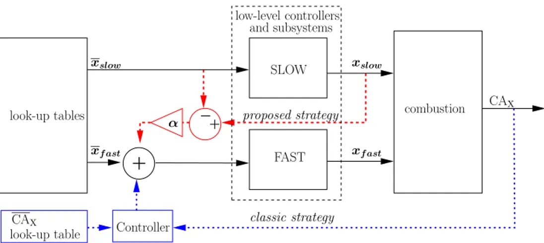
low-level controllers and subsystems FAST SLOW look-up tables Contribution of this thesis CAX 𝒙𝒔𝒍𝒐𝒘 𝒙𝒇 𝒂𝒔𝒕 𝒙𝒇 𝒂𝒔𝒕 combustion 𝒙𝒔𝒍𝒐𝒘

Figure 2: Combustion as the output of parallel slow and fast dynamical systems. The control variables (airpath, fuelpath, ignitionpath) are fed by look-up tables

assuming steady-state operation. 𝒙𝒔𝒍𝒐𝒘: slow variables, 𝑥𝑓 𝑎𝑠𝑡: fast variables,

𝒙𝒔𝒍𝒐𝒘 and 𝑥𝑓 𝑎𝑠𝑡: the tracked setpoints of 𝒙𝒔𝒍𝒐𝒘 and 𝑥𝑓 𝑎𝑠𝑡, CAX: control tar-get. Each variable has an individual low-level controller. The proposed control

methodology (red line) compensates for sluggishness in the 𝒙𝒔𝒍𝒐𝒘 variables by

acting on the 𝑥𝑓 𝑎𝑠𝑡 variables. control.

Combustion control is usually achieved with a static, open-loop method (as-suming steady-state operation). Accurate look-up tables are calculated for the steady-state using reference test benches in order to determine an optimal

trade-off between the various effects of CAX (torque production, pollutant emissions,

noise). Addressing only steady-states limits the calibration effort, but the result-ing look-up tables do not account for sharp transients. These transients cannot be represented as a quasi-static sequence of equilibria. Unfortunately, transients are frequently encountered in reference cycles (e.g. the American driving cycle (FTP, see [66]) or the New European Driving Cycle (NEDC, see [17])) and under

real road conditions. When transients occur, the CAX variables will

systemati-cally drift away from the optimal values determined for steady operation. As will now be shown, this effect can be attributed to differences in the settling times of the various subsystems constituting the engine.

Combustion is dependent on numerous variables: thermodynamic conditions

in the chamber (pressure (𝑃𝑐𝑦𝑙), temperature (𝑇𝑐𝑦𝑙)), composition of the mixture

(air mass (𝑚𝑎𝑖𝑟), fuel mass (𝑀𝑓), and burned gases mass (𝑚𝑏𝑔)), and combustion

phasing (which is governed by fuel injection timing in CI engines and by a spark in SI engines). The first two categories define what is burned, while the last one determines how it is burned. In all classical engine control setups, these variables are managed by individual low-level controllers. This separation is motivated by the need for simplicity, ease of tuning, and a general preference for decoupling strategies. However, two separate sets of variables should be distinguished on the

basis of their dynamic response.

- Slow variables (𝒙𝒔𝒍𝒐𝒘). Gas masses and temperatures are the result of

inherently slow processes such as gas propagation (through pipes), actuator constraints (such as variable valve actuation), and thermal exchange. These variables, among others, have slow dynamics (with typical settling times of 1 s) and cannot be accelerated.

- Fast variables (𝑥𝑓 𝑎𝑠𝑡). The ignition and injection times, for example, are

variables that do not depend on macroscopic dynamics. They can be freely varied from one engine cycle to the next.

This research represents combustion as a combination of slow and fast processes, referred to hereafter as the slow/fast paradigm. The general scheme of the com-bustion process is shown in Figure 2. Independent controllers guarantee that both 𝒙𝒔𝒍𝒐𝒘 and 𝑥𝑓 𝑎𝑠𝑡 track their desired steady-state values 𝒙𝒔𝒍𝒐𝒘 and 𝑥𝑓 𝑎𝑠𝑡, which are stored in static look-up tables. Since the actual values become inconsistent

dur-ing transients, however, the combustion phasdur-ings {CAX}0≤𝑋≤100 acquire large

deviations from their desired behavior whenever transients occur.

Among the possible combustion phasings ({CAX}0≤𝑋≤100), we pick a single

variable of particular interest. For brevity, we denote it CAX(this is now a scalar,

e.g. CA10 or CA50).

Interestingly, changes in the scalar variable 𝑥𝑓 𝑎𝑠𝑡can compensate for

sluggish-ness and offsets during the settling time of the vector 𝒙𝒔𝒍𝒐𝒘. More precisely, since

the calibrated look-up tables lead to optimum combustion and optimum values

for the combustion phasings CAX, we propose modifying the fast variable control

strategy to ensure that the combustion phasing exactly tracks its optimum value during transients in spite of lag in the slow variables. If the chosen combustion

phasing CAX can be made equal to its optimum value CAX, the whole

combus-tion process will be closer to its optimum behavior during a transient. Indeed, we claim that under this control scheme torque production, pollution and noise will be as close as possible to their optimal trade-off values defined in the steady-state.

To determine which control actions should be performed on the 𝑥𝑓 𝑎𝑠𝑡 variable,

we use a phenomenological model of the combustion process. The model is a set of differential systems solved over variable time intervals implicitly defined by

varying boundary conditions. Temporal tracking errors in the 𝒙𝒔𝒍𝒐𝒘 variables are

represented as offsets in the initial conditions, allowing us to formulate and solve a target reaching problem.

This type of model-based control complements the static look-up tables. In-terestingly, this approach does not require any in-cylinder sensor, and therefore corresponds to a dynamic open-loop control. The method presented here signif-icantly improves the transient control of combustion through a combination of simple off-line computations and real-time on-line computations making use of the look-up tables that already exist. No additional calibration is required.

nited (SI) and Compression Ignition (CI) engines. The manuscript is organized as follows. In Chapter 1, we provide the necessary background on SI and CI engines along with our motivations for addressing combustion phasing control by means of the slow/fast paradigm. We also describe existing control architectures and sort the variables involved in combustion into slow and fast subsets. In Chap-ter 2, we propose a general control strategy and compare its principles against the state of the art. A general formulation of compression/combustion models is proposed and used to derive a general controller synthesis. Finally, Chapters 3, and 4 give case studies of SI and CI engines respectively. Numerous simulations and experimental results are discussed, stressing the success and relevance of this approach.

Notations and acronyms

Acronyms

BGR Burned Gas Ratio

CA Crankangle

CAX Crankangle at which X% of fuel mass is burnt

CAI Controlled Auto-Ignition (engine)

CI Compression Ignition (engine)

CO Carbon Monoxide

ecf End of Cool Flame

ECE Urban driving cycle

EGR Exhaust Gas Recirculation

EUDC Extra-Urban Driving Cycle

FAR Fuel to Air Ratio

FTP Federal Test Procedure

HC Unburned Hydrocarbons

HCCI Homogeneous Charge Compression Ignition (engine)

HP EGR High Pressure Exhaust Gas Recirculation

IC Internal Combustion (engine)

IMEP Indicated Mean Effective Pressure

ivc Intake Valve Closure

KIM Knock Integral Model

LP EGR Low Pressure Exhaust Gas Recirculation

MFB Mass Fraction of Burned fuel, ranges from 0 to 1

NADI Narrow Angle Direct Injection

NEDC New European Driving Cycle

NO𝑥 Nitrogen Oxides

ROHR Rate Of Heat Released

SI Spark Ignition (engine)

sit Spark Ignition Timing

soc Start Of Combustion

soi Start Of Injection

TDC Top Dead Center

VVT Variable Valve Timing

Function regularity classes

𝐶0 _{continuous functions}

𝐶1 _{continuously differentiable functions}

𝐶0_{∩ 𝐶}1

𝑝𝑐 continuous and piecewise continuously differentiable functions

General Notations

In the manuscript, vectors are in bold lowercase and matrices in bold upper-case. Scalars are either lower- or uppercase non-bold. A variable with an overline 𝑥 is the reference variable corresponding to the variable 𝑥.

Symbol Quantity Unit

𝜃 Crankangle ∘_CA

𝜃𝑇 𝐷𝐶 top dead center crankangle ∘CA

𝑉 (𝜃) Cylinder volume m3

𝑃 (𝜃) Cylinder pressure Pa

𝑇 (𝜃) Cylinder temperature K

𝑋 In-cylinder burned gas ratio (BGR)

-𝑇𝑤 _{Cylinder wall temperature K}

𝑇𝑤

𝑖𝑣𝑐 Cylinder wall temperature at ivc K

𝑉𝑖𝑣𝑐 In-cylinder volume at 𝑖𝑣𝑐 m3

𝑃𝑖𝑣𝑐 Cylinder pressure at 𝑖𝑣𝑐 Pa

𝑇𝑖𝑣𝑐 Cylinder temperature at 𝑖𝑣𝑐 K

𝜙 Fuel/air ratio

-𝜙𝑠 Stoichiometric fuel/air ratio

-𝜃𝑖𝑛𝑗 Injection crankangle ∘CA

𝜃𝑠𝑜𝑐 Start of combustion crankangle ∘CA

𝛾 Ratio of specific heat

-𝑇𝑞 Torque Nm

𝑁𝑒 Engine speed rpm

𝒙𝒔𝒍𝒐𝒘 Slow variables *

𝑥𝑓 𝑎𝑠𝑡 Fast variable *

𝑥𝑙𝑜𝑎𝑑 Entry of the fast variable look-up table *

𝒑𝒊𝒗𝒄 Airpath driven in-cylinder conditions at ivc *

𝒑𝒊𝒗𝒄 In-cylinder conditions at ivc *

ℳ Formal model giving the CAX ∘CA

Symbol Quantity Unit

𝜶 Proposed correction gain *

ℎ𝑐 Heat transfer coefficient

𝑄𝐿𝐻𝑉 Fuel low heating value J/kg

𝜂𝑣𝑜𝑙 Volumetric efficiency

-Notations for the SI engine case study

Symb. quantity Unit

𝜃sit sit crankangle ∘CA

𝑉𝑚𝑖𝑛

𝑓 𝑙 Minimal flame volume (initiation of the flame) m3

𝑇𝑢(𝜃) Unburned zone temperature K

𝑀𝑖𝑣𝑐 In-cylinder total mass of gas at ivc (air & burned gas)

-𝑚𝑎𝑖𝑟 Aspirated air mass kg

𝑚𝑒𝑠𝑡

𝑎𝑖𝑟 Estimated aspirated air mass kg

𝑀𝑓 Injected fuel mass kg

𝑥𝑓 MFB

-𝜌𝑢 Unburned zone density kg/m3

𝑌𝑢 Unburned zone fuel mass fraction

-𝑈 Laminar burning speed m/s

𝑈0 Laminar burning speed at ambient conditions m/s

𝑊𝑡 Turbulent wrinkling

-𝐴 Piston head surface m2

𝑆𝑓 𝑙 Flame surface area m2

𝑆𝑔𝑒𝑜 Geometric flame surface area (without wrinkling) m2

𝑇𝑎𝑚𝑏 Ambient temperature ∘K

𝑃𝑎𝑚𝑏 Ambient pressure Pa

𝛼 Constant appearing in the laminar burning speed

-𝛽 Constant appearing in the laminar burning speed

-𝑉𝑢 Unburned zone volume m3

𝑀𝑢 Mass of the gases in the unburned zone kg

𝑘 Density of turbulent kinetic energy Js/kg

𝑓𝑤𝑎𝑙𝑙 Wall destruction term of the flame propagation J

𝐸𝑘𝑖𝑛 Kinetic energy associated with the tumbling J

𝛿𝑥 Characteristic function (1 if x is true, 0 otherwise)

-𝑥𝜃𝑖𝑣𝑐 Artificial state representing 𝜃𝑖𝑣𝑐

∘ CA

𝑥𝑀𝑖𝑣𝑐 Artificial state representing 𝑀𝑖𝑣𝑐 𝑘𝑔

𝑥𝑡𝑢𝑚𝑏𝑙𝑒 Artificial state representing 𝑁𝑖𝑣𝑐𝑡𝑢𝑚𝑏𝑙𝑒

-𝑥𝑀𝑓 Artificial state representing 𝑀𝑓 kg

-𝑁_𝑖𝑣𝑐 Tumble number initial value -𝑁𝑡𝑢𝑚𝑏𝑙𝑒

𝑒𝑚𝑝 Empirical look-up table of the tumble initial value

-Notations for the CI engine case study

Symbol Quantity Unit

𝜃𝑠𝑜𝑐 Start of combustion crankangle ∘CA

𝜃𝑒𝑐𝑓 End of the cool flame crankangle ∘CA

𝒜𝑎𝑖 _{Integrand function of the auto-ignition model (KIM)}

-𝒜𝑐𝑓 _{Integrand function of the cool flame model (KIM)}

-𝑝(𝜃) In-cylinder thermodynamic parameters vector *

𝑃𝑖𝑛𝑡 Intake manifold pressure Pa

𝑇𝑖𝑛𝑡 Intake manifold temperature ∘K

𝑋𝑖𝑛𝑡 Intake manifold BGR Pa

𝜏𝑎𝑖 Artificial state for the evolution of the auto-ignition

-𝜏𝑐𝑓 Artificial state for the evolution of the cool flame

-𝑀𝑓 Total injected fuel mass kg

𝑀_𝑓𝑝𝑖𝑙𝑜𝑡 Injected fuel mass during the pilot injection kg

𝑀𝑚𝑎𝑖𝑛

𝑓 Injected fuel mass during the main injection kg

Chapter 1

A description of transient

combustion control issues

There exists two main classes of automotive engines each of which generates torque by burning a blend of air, fuel, and exhaust gases. The first of these, the Compression Ignition (CI) engine, initiates combustion by compressing the gaseous fuel mixture. This class includes ordinary Diesel engines [23], Homoge-neous Combustion Compression Ignition (HCCI) Diesel engines [68], and HCCI gasoline engines (also referred to as Controlled auto ignition (CAI)). The second type, the Spark Ignited (SI) engine, initiates combustion in the chamber with a correctly timed spark. This class comprises classic gasoline engines [23] and natural gas engines. Apart from these differences, both types of engines operate quite similarly and, consequently, require similar engine controls.

We now present these two classes of engines. We detail their various con-stituting subsystems (airpath, fuelpath, and ignition path for SI engines), along with their respective timescales and usual controllers. For each class, we sketch

the usually observed transient behavior for CAX variables, stress their flaws, and

exhibit the slow/fast variables that play key roles in the in-cylinder combustion.

1.1

Background on SI engine

1.1.1

General engine structure

Internal combustion engines for which the combustion can be directly initiated by a spark are designated as SI engines. A pictorial view of the combustion chamber along with neighboring elements (the spark plug, the injector, the intake and exhaust valves, the intake and exhaust manifold, and the cylinder) is given in Figure 1.1. Details can be found in [23]. In the case of four strokes engines, the engine functioning timeline is the following:

1. Intake phase (cylinder filling): the intake valve opens and the fresh air en-ters the cylinder while the piston goes down. This phase lasts until the intake valve closes (this particular time is called ivc: intake valve closing). If available, Variable Valve Actuation (VVA) may modify the breathing of the engine (by impacting on the opening and closing of the intake and ex-haust valves). This permits to re-aspirate some of the preceding combustion burned gases from the exhaust line. The fuel is injected during this phase. 2. Compression phase: the piston goes up and compresses the aspirated air,

burned gases and fuel.

3. Combustion phase: the spark plug generates a spark that initiates the com-bustion of the blend of air/burned gases/fuel. A flame propagates in the chamber freeing the fuel chemical energy. The pressure increases and pushes back the piston.

4. Exhaust phase: once the piston has completed its descent, the exhaust valve opens. The exhaust gases are then flushed out of the cylinder towards the exhaust line. exhaust manifold Injector Spark plug actuator

Intake valve Exhaust valve

actuator cylinder wall piston combustion chamber exhaust valve intake valve intake manifold

Figure 1.1: View of the combustion chamber along with the surrounding devices. This timeline is pictured in Figure 1.2 where each phase is represented along with the actuators acting during them. In view of ecological concerns and to improve the engine performances, modern SI engines are equipped with turbocharger(s) and VVA. The turbocharger(s) permits to increase the engine power by increasing the pressure (and thus the aspirated air mass) in the cylinder. The VVA permits to change the intake and exhaust valves lift and their timing. In fact, VVA allows

1.1. BACKGROUND ON SI ENGINE Compression injection actuators throttle Cylinder filling Spark plugs spark Exhaust timeline exhaust valve opening

Airpath variable valve act.

Timeline available _{turbocharger(s)} Injectors Fuelpath Airpath Ignitionpath Combustion (ivc)

intake valve closing

Figure 1.2: SI engine functioning timeline. Each phase lasts 20 ms at 1500 rpm. exhaust gases from the preceding combustion to be re-aspirated into the cylinder and mixed with fresh air.

The general structure of a SI engine is given in Figure 1.3. It can be di-vided into three main subsystems. First, the airpath which consists of all the pipes, turbocharger(s), intake throttle, intake and exhaust manifolds, VVA sys-tems and heat exchangers. The airpath feeds the cylinder providing appropriate thermodynamic and physical conditions. In fact, all the airpath devices act on the combustion by creating these conditions at the ivc moment (this moment is noted 𝜃𝑖𝑣𝑐). After 𝜃𝑖𝑣𝑐, the cylinder is isolated from the airpath until the exhaust phase.

Then, the fuelpath, which consists of the injection system, is used to inject the appropriate fuel mass into the cylinder at the appropriate time.

At last, the ignitionpath which consists of the spark plugs, provides a spark inside the cylinder to initiate the combustion.

After the ivc, the fuelpath and the ignitionpath are the only control variables to act on the combustion.

1.1.2

SI engine control

Over the years, numerous airpath controllers have been designed (see [37, 48, 62]). The task of such controller is to make the airpath feed the cylinder with the right thermodynamic properties at ivc with the right valve timings. Among these parameters, the air mass plays the most important role (see below the de-scription of the fuelpath control). The main task of the airpath controller is thus to track the aspirated air mass setpoint. To this end, static maps of the values of the thermodynamic conditions at ivc (gathered in a vector of parameters noted

𝒑𝒊𝒗𝒄) and of the variable valve actuator positions are used (and, among those,

the ivc timing which plays a great role as will appear in the following). How-ever, due to the inertia of the physical devices (hold-ups in pipes, turbochargers, variable valve actuators) and the natural saturations of the mechanical systems involved, the tracking of these setpoints cannot be rendered arbitrarily fast (the

Turbocharger VVA Exhaust valve VVA Compressor Throttle Injector Spark Turbine Intercooler

Intake manifold Exhaust manifold

plug

Intake valve

Figure 1.3: Scheme of a general SI engine equipped with direct injection, VVA and a turbocharger.

airpath bandwidth is approximately 1 Hz). Tracking errors may also happen due to airpath malfunctions such as natural device ageing. In fact, since the ther-modynamic conditions are not a free set of variables (e.g. they are related by the ideal gas relation), it is not possible to control them independently. Thus, only a reduced set of parameters is actually controlled by the airpath controller (and thus mapped), and the other one can be computed using the static relation holding between them. In SI engines, the actually controlled variables usually include the air mass, the gas composition (BGR) and the VVA positions, while for instance, the burned gases mass can be inferred using the composition and the air mass. However, for sake of simplicity of the exposition, but without loss

of generality, we consider in the following that all thermodynamic variables (𝒑𝒊𝒗𝒄)

are controlled by the airpath.

The fuelpath controller regulates the fuel injection. To maximize the efficiency of exhaust gases after-treatment devices, the FAR (𝜙) has to be maintained as

close as possible to the stoichiometric value (𝜙𝑠) (see [19, 65]). Accordingly, the

injected fuel mass 𝑀𝑓 is directly computed from the (estimated) value of the

in-cylinder air mass 𝑚𝑒𝑠𝑡𝑎𝑖𝑟 (𝑀𝑓 = 𝜙𝑠𝑚𝑒𝑠𝑡𝑎𝑖𝑟). This estimate is usually provided by an air mass observer in the airpath controller. Feedback controllers using exhaust FAR sensors may also be considered. To maximize the mixture homogeneity, injection usually takes place during the intake phase. Fuel vaporization and mixing with air and burned gases are both completed before ignition. The injection timing has no major impact on the combustion phasing. This is the major difference between SI and CI engines. Its effect is in fact visible on pollutant formation (through the mixture homogeneity). The best control strategy results from a tradeoff. A too early injection causes the fuel to stick onto the piston head, while a too late injection reduces the available time for homogenization. We do not

1.1. BACKGROUND ON SI ENGINE want to modify this tradeoff. Consequently, controlling the injection timing in SI engines is left out of the scope of the thesis.

The torque production level does not exclusively depend on the amount of injected fuel and air mass. Spark timing, which initiates the combustion, plays a key role in the quality of the combustion (both in terms of efficiency and pollutant generation). A “global” criterion commonly used to evaluate the quality of the

combustion is the middle of the combustion (CA50) [15]. In fact, one considers

that the engine is working at its maximal efficiency when the CA50 is reached

at an optimal timing noted CA50. The role of the ignitionpath controller is thus

to make the CA50 track the optimum value CA50, by adjusting the ignition time

𝜃sit according to look-up tables. Due to the overwhelming number of parameters

influencing the combustion kinetics, they cannot all be used as inputs of these

tables. A tradeoff is usually met by using the engine speed 𝑁𝑒 and the drivers

torque demand as entries1_{. The parameters that are not taken into account, such}

as the temperature of the in-cylinder gases or the BGR, are assumed to be close to their steady-state value corresponding to the tracked operating point.

Torque Demands

Driver

injectors

Static

maps spark plugs

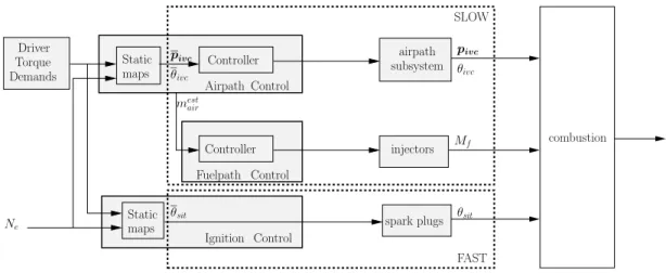
Static maps Controller 𝒑𝒊𝒗𝒄 Control Fuelpath 𝑀𝑓 𝑁𝑒 Ignition Control 𝜃sit Control Airpath 𝜃sit SLOW FAST Controller 𝑚𝑒𝑠𝑡 𝑎𝑖𝑟 𝒑𝒊𝒗𝒄 𝜃𝑖𝑣𝑐 𝜃𝑖𝑣𝑐 combustion airpath subsystem

Figure 1.4: Classic SI engine control architecture. 𝒑𝒊𝒗𝒄 are the thermodynamic

and physical composition in the cylinder at ivc. 𝒑𝒊𝒗𝒄 is the steady-state mapped

value of 𝒑𝒊𝒗𝒄. 𝑀𝑓 is the injected fuel mass. 𝜃𝑖𝑣𝑐 is the ivc timing and 𝜃𝑖𝑣𝑐, its

steady-state mapped value. 𝜃sit is the spark timing and 𝜃sit, its steady-state

mapped value. The fuelpath is fed with an estimate of the in-cylinder air mass (𝑚𝑒𝑠𝑡

𝑎𝑖𝑟) usually provided by the airpath controller. The slow subsystem consists

of the airpath and the fuelpath, while the fast subsystem is the ignitionpath.

1

The second usually met solution is to feed the steady-state map with the engine speed and the aspirated air mass. This is considered as an extension of the proposed branching scheme and is treated in § 2.5.2.

1.1.3

Combustion phasing transient behavior

We now describe the behavior of the presented classic controllers during tran-sients and their impact on the combustion phenomenon. During trantran-sients, the airpath controller concentrates on the air mass control. It regulates the in-cylinder thermodynamic variables so that they track their setpoints. However, since the airpath cannot be accelerated as much as desired, there exists temporary mis-matches which, in fact, negatively impact on the combustion efficiency. Mainly, the culprit is the ignitionpath controller which ignores these mismatches, and

sim-ply applies an open-loop control value 𝜃sit for the ignition time based on look-up

tables assuming in-cylinder thermodynamic variable have already reached their expected steady-state values. This issue is worsened on engines equipped with

VVA. Indeed, the VVA actuators play an important disturbing role2_{. The VVA}

actuators changes the valves lift and their timing to create internal EGR which dilutes the air charge (and thus slows down the flame propagation [23]). Besides these beneficial effects, changing the valve lift also has an impact on the turbu-lence in the chamber. The flame propagation, which depends on this turbuturbu-lence, is then either accelerated or slowed down. During transients, the effects of burned gases, pressure, temperature, and VVA disturbance on the flame propagation are significant. One can expect to improve the quality of the combustion (in terms of consumption) by compensating the offsets of in-cylinder thermodynamic and physical (VVA positions) parameters using the spark ignition time.

In summary, the general structure of a SI engine controller is depicted in Figure 1.4. The variables influencing the combustion can be split into two cat-egories: the slow variables (vector) are 𝒙𝒔𝒍𝒐𝒘 = (𝒑𝒊𝒗𝒄, 𝑀𝑓, 𝜃𝑖𝑣𝑐) and the (scalar) fast variable is 𝑥𝑓 𝑎𝑠𝑡 = 𝜃sit.

1.2

Background on CI engine

1.2.1

General engine structure

Internal combustion engines for which the combustion is initiated by the com-pression of the mixture are designated as Comcom-pression Ignited (CI) engines. The combustion chamber can be pictured as in Figure 1.1, except that there is no spark plug. In the cases of four strokes engines, the engine functioning timeline is the following:

1. Intake phase (cylinder filling): the intake valve opens and the fresh air enters the cylinder while the piston goes down. This phase lasts until the intake valve closes (ivc). Exhaust Gas Recirculation (EGR), if present, modifies the composition of the gases aspirated through the intake valve by 2

Additionally, the VVA actuators can also be used to speed up the airpath dynamics, which in turn, introduces further offsets from the expected steady-state.

1.2. BACKGROUND ON CI ENGINE extracting exhaust gases in the exhaust line and mixing them with the fresh air in the intake line. If available, VVA may modify the breathing of the engine (intake and exhaust valves). This permits to re-aspirate some of the preceding combustion burned gases directly from the exhaust line through the exhaust valve).

2. Compression phase: the piston goes up and compresses the aspirated air and burned gases. The fuel is injected during this phase.

3. Combustion phase: after a delay depending on the thermodynamic and physical conditions (the so-called auto-ignition delay), the blend of air/burned gases/fuel auto-ignites. The combustion frees the fuel chemical energy. The pressure increases and pushes back the piston.

4. Exhaust phase: once the piston has completed its descent, the exhaust valve opens. The exhaust gases are then flushed out of the cylinder towards the exhaust line.

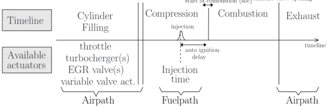
This timeline is pictured in Figure 1.5 where each phase is represented along with the various available actuators acting.

delay Available

actuators

Intake valve closing (ivc) Compression

injection

start of combustion (soc)

Injection time Combustion _Exhaust throttle turbocherger(s) EGR valve(s) Airpath Fuelpath Filling Cylinder Timeline

exhaust valve opening

timeline

Airpath

auto ignition

variable valve act.

Figure 1.5: CI engine functioning timeline. Each phase lasts 20 ms at 1500 rpm. The general structure of a CI engine is represented in Figure 1.6. It can be divided into two main subsystems. First, the airpath which consists of all the pipes, turbocharger(s), intake throttle, EGR valve(s), exhaust back pressure valve, intake and exhaust manifolds, VVA systems and heat exchangers. The airpath feeds the cylinder and provides appropriate thermodynamic and physical conditions. In fact, all the airpath devices act on the combustion by creating these conditions at the ivc instant. After ivc, the cylinder is isolated from the airpath. Secondly, the fuelpath which consists of the injection system. It injects the appropriate mass of fuel at the appropriate time in the chamber. After the ivc, the fuel injection parameters are the only control variables acting on the combustion.

back pressureexhaust valve actuator Intake VVT _{Exhaust VVT} actuator Injector Turbine Intercooler Intake manifold Throttle Exhaust manifold EGR HP valve Compressor EGR LP valve

Figure 1.6: Scheme of a general four cylinder CI engine. It is equipped with direct injection, a VVA, a low Pressure EGR (LP EGR) recirculation, a high pressure EGR (HP EGR) recirculation, an exhaust back pressure valve, an intercooler, and a turbocharger.

1.2.2

CI engine control

As a result of this physical/temporal separation, usual CI engine controllers are classically consisting of two distinct controllers aiming at controlling each of these subsystems.

The task of the airpath controller is to make the airpath feed the cylinder with the right thermodynamic properties at ivc with the right valve timings (and

among those the ivc timing 𝜃𝑖𝑣𝑐). To this end, static maps of the values of the

thermodynamic conditions at ivc (gathered in a vector 𝒑𝒊𝒗𝒄) and of the valve

timings are used. These 2D-maps usually have the drivers torque request and actual engine speed as inputs. In this thesis, it is assumed that such a properly working airpath controller is already installed on the engine, which allows reason-able tracking of the setpoints values (such controllers can be found in [9, 46, 67] and the references therein). However, due to recirculation holds-up, inertia of the physical devices (turbochargers, variable valve actuators), and actuators sat-uration, the tracking of these setpoints cannot be rendered arbitrarily fast (the airpath bandwidth is approximately 1 Hz). Tracking errors may also happen due to airpath malfunctions such as EGR valve clogging or natural device ageing. In fact, as in SI engines, since the thermodynamic conditions are not a free set of variables (they are, at least approximatively, related through the ideal gas law for instance), only a reduced set is actually controlled by the airpath controller (and thus mapped), while the other one can be inferred from the static rela-tion holding between them all. In CI engines, these actually controlled variables usually include the pressure, composition, and VVA positions while for instance, the burned gases mass or the air mass can be determined using the composition

1.2. BACKGROUND ON CI ENGINE 340 360 380 400 4.5 5 5.5 6 CA50 IM E P [b a r] (a) Torque 340 360 380 400 85 90 95 100 CA50 No is e [d B ] (b) Noise 3400 360 380 400 20 40 60 CA50 C O [g / k W h ] (c) Carbon monoxide 3405 360 380 400 10 15 20 CA50 HC [g / k W h ] (d) Unburned hydrocarbons 3400 360 380 400 1 2 3 CA50 NO x [g / k W h ]

(e) Nitrogen oxides

3401 360 380 400 2 3 4 5 CA50 S m o k e [F S N] (f) Smoke

Figure 1.7: Experimental results obtained for a four-cylinder CI Diesel engine (HCCI): influence of the combustion phase (represented by varying values of

CA50) on engine pollutants, noise, and torque production. The combustion

phasings are the only parameters varying during the experiment (in fact, the injection timing is used to delay or to bring forward the whole combustion pro-cess); the Burned Gas Ratio (BGR), intake manifold pressure, intake manifold

temperature, and injected fuel mass are constant. 360∘_{CA represents the TDC.}

and the ideal gas relation. However, for sake of simplicity, in the following, we

consider that all thermodynamic variables (𝒑𝒊𝒗𝒄) are controlled by the airpath.

On the other hand, classic fuelpath controllers are as follows. During the cylin-der compression phase, fuel is injected and mixed with the compressed air and burned gas mixture. The fuel vaporizes and auto-ignites after the auto-ignition delay. Standard fuelpath control strategies focus on controlling the injected fuel mass and the injection timing. The direct injection technology enables to change these parameters from one cycle to the next. In practice, the injected fuel mass is directly computed from the driver’s torque request. Therefore, this strategy cannot be changed without seriously jeopardizing the engine performance. Conse-quently, the fuel mass control is left as-is in the strategy we propose. By contrast,

the injection timing (noted 𝜃𝑖𝑛𝑗 for start of injection) is a direct trigger acting

on the combustion phasing3_{. Classically, to control the injection timing,}

opti-mal values are determined at steady-state on experimental test-benches. These 3

In this chapter, and, if not told otherwise in the following ones, we only consider mono-pulse injection. The discussion on multi-pulse injection is postponed until Section 4.2.

represent a tradeoff between efficiency, pollutant emissions and noise. To illus-trate this, Figure 1.7 shows experimental variations of the combustion phasing created by variations of the injection timing (while all other influencing variables are kept constant). It clearly appears that the optimal value can only be an arbi-trary tradeoff between torque, noise and pollutant emissions. Once determined, these optimal values are stored into 2-D look-up tables using the engine speed and the driver’s torque request as inputs.

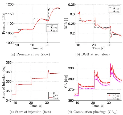
10 20 30 1000 1050 1100 1150 1200 Time [s] P re ss u re [h P a ] Pivc Pivc

(a) Pressure at ivc (slow)

10 20 30 0.2 0.25 0.3 0.35 Time [s] B G R [-] Xivc Xivc (b) BGR at ivc (slow) 10 20 30 345 350 355 360 365 Time [s] S ta rt o f In je ct io n [d eg ] θsoi θsoi

(c) Start of injection (fast)

10 20 30 360 370 380 390 Time [s] C A [d eg ] CA50 CA10

(d) Combustion phasings (CAX)

Figure 1.8: Experimental transient results on a 4-cylinder CI engine (HCCI) at a constant speed of 1500 rpm. Evolution of the initial thermodynamic condi-tions in the cylinder at ivc (pressure and temperature, both considered as slow variables), the start of injection (a fast variable) and the combustion phasing (combustion performance index). During transients, the combustion phasing

CAX features large overshoots due to the temporary mismatch between slow

and fast variables. 360∘_{CA represent the TDC. In these figures, 𝑃}

𝑖𝑣𝑐 and 𝑋𝑖𝑣𝑐 are computed according to the assumptions of § 4.1.2

1.3. SLOW/FAST SCHEME FOR INTERNAL COMBUSTION ENGINES

1.2.3

Combustion phasing transient behavior

During transients, due to the airpath slow dynamics, the initial

thermody-namic conditions in the cylinder 𝒑𝒊𝒗𝒄 and valve timing 𝜃𝑖𝑣𝑐4 do not match their

optimal steady-state values. Since the injection timing 𝜃𝑖𝑛𝑗 does not take into

account these parameters, the fuel is injected as if the steady-state was reached. Then, the combustion does not occur at the right timing. This is clearly visible in Figure 1.8 where experimental transients obtained on a CI engine are reported. In details, the evolution of two cylinder initial conditions (pressure and BGR, which transient behavior is slow), of the injection timing (which can be changed

from one cycle to the next), and the resulting combustion phasings (CA10 and

CA50) are depicted. The combustion phasing is shown to deviate away from its

steady-state value during transients. Thus, the combustion phasing theoretical optimal tradeoff is not satisfied during transients.

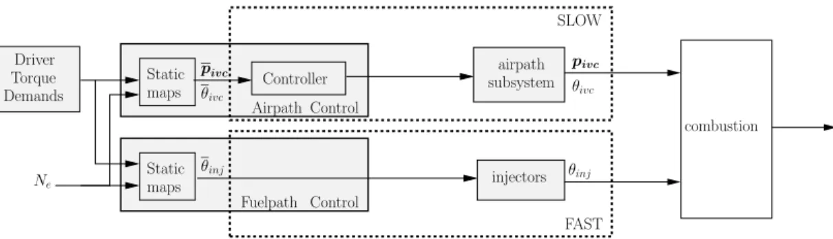
To summarize the above discussion, the general structure of a CI engine

controller is depicted in Figure 1.9. The slow (vector) variables are 𝒙𝒔𝒍𝒐𝒘 =

(𝒑𝒊𝒗𝒄, 𝜃𝑖𝑣𝑐)𝑇 and the fast (scalar) variables is 𝑥𝑓 𝑎𝑠𝑡 = 𝜃𝑖𝑛𝑗.

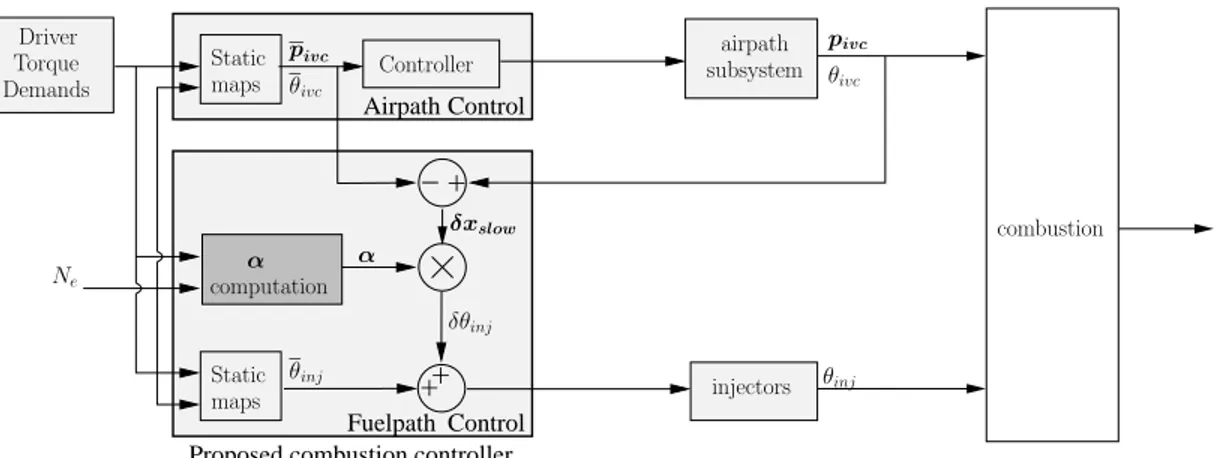
Demands Driver Static maps Static maps

Controller _subsystemairpath

𝒑𝒊𝒗𝒄 Airpath 𝒑_𝒊𝒗𝒄 𝜃𝑖𝑛𝑗 𝑁𝑒 𝜃𝑖𝑣𝑐 𝜃𝑖𝑣𝑐 Control Control Fuelpath 𝜃𝑖𝑛𝑗 SLOW FAST combustion injectors Torque

Figure 1.9: Classic CI engine control architecture. 𝒑𝒊𝒗𝒄 are the thermodynamic

and physical conditions in the cylinder at ivc. 𝒑𝒊𝒗𝒄 is the mapped steady-state

value of 𝒑𝒊𝒗𝒄. 𝜃𝑖𝑣𝑐 is the ivc timing and 𝜃𝑖𝑣𝑐, its steady-state mapped value. 𝜃𝑖𝑛𝑗 is the injection timing, and 𝜃𝑖𝑛𝑗 are the mapped steady-state value of 𝜃𝑖𝑛𝑗. Both the airpath and the fuelpath subsystems work in parallel without any noticeable influence on each other. One is slow, and one is fast. As a result, during transients, the combustion timing deviates from its optimum.

1.3

Slow/fast scheme for internal combustion

engines

After having presented the classic control architectures of the SI and CI en-gines, we now wish to underline that they both suffer from the same flaw resulting

4

this may be due to actuator constraints, or, as in SI engines, due to a particular transient control strategy aiming at speeding up some other thermodynamic conditions transients.

in poor combustion control during transients. In both cases, we have emphasized the presence of slow and fast variables. The “slow controller” (airpath and

fuel-path controllers in SI engines, airfuel-path controller in CI engines) makes the 𝒙𝒔𝒍𝒐𝒘

variables follow their setpoint 𝒙𝒔𝒍𝒐𝒘. In fact, all the variables included in the

vector 𝒙𝒔𝒍𝒐𝒘 are not actually controlled since there exist static relations between

them (such as the ideal gas relation or the stoichiometric combustion in SI en-gines). However, since the static relations are fully known, we consider in the

following that the whole vector 𝒙𝒔𝒍𝒐𝒘 is controlled even if only a reduced set of

them is actually controlled5_{. Among the 𝒙}

𝒔𝒍𝒐𝒘 variables, 𝜃𝑖𝑣𝑐 plays a significant role since it separates the intake phase and the compression/combustion phases. This tracking performance suffers from the relative sluggishness of the slow subsystem and exhibits offsets during transients. Consequently, the combustion

phasing is degraded and exhibits over- and undershoots6_{. Interestingly, in both}

engines architectures, the fast variable has a strong impact on combustion phasing since it directly (in SI engines) or indirectly (through the auto-ignition delay in CI engines) controls the beginning of the combustion and thus of the whole combustion phasing. Moreover, the slow variables can be simply inferred from measurements, identification and/or observation. It follows that one can use the

fast variables 𝑥𝑓 𝑎𝑠𝑡to compensate for the slow evolution of the known parameters

𝒙𝒔𝒍𝒐𝒘. This is the path we explore in this thesis. It is detailed in the next chapter.

5

The other variables naturally converge to a vector 𝒙𝒔𝒍𝒐𝒘 gathering the actually mapped reference value for the smaller set of variables and reference values for the other variables that can be easily computed using the static relations.

6

In fact, each variable in this group has its own dynamics and settling time. For instance, the process of gas filling the in-cylinder involves two of these variables (the masses of air and burned gas), so it depends on two distinct (and long) settling times. It may be possible to speed up some of the slow variables by coordinating the respective low-level controllers of these variables, at the expense of the speed of other variables such as temperature. This is actually a subject of ongoing research. Interested reader can refer to [47] for SI engines and [46] for Diesel engines.

Chapter 2

Proposed model-based

combustion controller

To improve the existing controllers exposed in Chapter 1, which rely on static look-up tables under all circumstances, a control of the combustion phasing is

now proposed.It will be of particular interest during transients. Let CAX be the

desired combustion phasing to control. It is considered that the calibration phase of the engine has led to the construction of steady-state maps storing optimal

values 𝑥𝑓 𝑎𝑠𝑡 and 𝒙𝒔𝒍𝒐𝒘 corresponding to an optimal combustion phasing CAX.

The goal of any combustion controller is then to guarantee that, even during

transients, the actual combustion phasing CAX tracks the optimal one. To this

end, two main solutions have been studied in the literature. The simplest one is to use feedback through in-cylinder measurements while the second one is to use a partially feedforward model-based control technique. After having presented them, we propose our own method.

2.1

Existing combustion timing control

strate-gies

2.1.1

Solutions relying on in-cylinder sensors

The first class of methods uses information from in-cylinder sensors. High-frequency in-cylinder sensors enable accurate closed loop control action. The additional information from these sensors allows the reconstruction of several combustion characteristics and the utilization of them as feedback information.

Among the available sensors, in-cylinder pressure transducers are the most flexible [56]. In practice, solutions requiring such a hardware upgrade have been successfully applied to CI and SI engines. We now briefly present such solutions.

In CI engines, cylinder pressure feedback has most often been considered for Homogeneous Charge Compression Ignition (HCCI) engines. Several con-trol actions can be considered. In [21], Haraldsson et al. present a closed-loop combustion control mechanism using variable compression ratio (VCR) as an ac-tuator. Changing the compression ratio directly impacts on the rise of pressure and temperature in the cylinder, not just during compression, but also during the auto-ignition and combustion phases. Thus, VCR can be used to control

CA50. In [2, 54], a solution using two fuels with different combustion

proper-ties is presented. CA50 can be regulated by changing the recipe of the mixture

to be injected. In [1, 8, 10, 55, 57], HCCI control results based on a variable valve actuation are presented. These solutions modify the charge temperature by trapping hot exhaust gases in the cylinder from one cycle to the next; the whole combustion process can thereby be delayed or advanced. In [18, 22, 69], a thermal management solution is reported. The intake manifold temperature is modified by changing the mixture of hot and cold air in the intake line. Once again, combustion, being sensitive to thermal changes, can be delayed or advanced.

In SI engines (e.g. [61, 73, 74]), closed loop controllers have been presented for the spark timing using cylinder pressure feedback.

Finally, besides pressure sensors, several other sensors have been considered to provide feedback information on the combustion. For example, accelerome-ters strapped onto the engine block [13, 38, 53] or crankshaft angular velocity sensors [12] have also been considered for CI Diesel engines. Ion-current sensors located in the spark plug [14, 16], crankshaft angular velocity sensors [7], and torque sensors [3] have been studied to control the spark timing of SI engines.

All these solutions can provide accurate control of combustion phasing, but also suffer from serious drawbacks [59]: they imply costly hardware (additional sensors are needed and their integration in the combustion chamber raises some technological challenges) and software (the information provided by these sensors needs high frequency treatment which is not possible in commercial-line electronic control units) upgrades and drift with time (this is notably true for cylinder pressure sensors, the most widely considered technology, since the thermodynamic conditions in the chamber are rather extreme).

2.1.2

Model-based control

Instead of using in-cylinder sensors, some authors have considered models

of the engine cycle from the ivc, to a desired combustion phasing CAX. The

model is usually subdivided into a compression model and a combustion model. These models may be explicit (e.g., the Wiebe models [70]), implicit (e.g., the knock integral model [63]), or based on differential equations such as ratio of heat release [6, 11]). In all cases, the goal is to relate the 𝒙𝒔𝒍𝒐𝒘 and 𝑥𝑓 𝑎𝑠𝑡 variables to the combustion phasing. We now detail such approaches.

2.1. EXISTING COMBUSTION TIMING CONTROL STRATEGIES

Consider CAX, for a particular 0 ≤ 𝑋 ≤ 100, the desired combustion phasing.

As mentioned earlier, it is presumed that the calibration phase of the engine has

led to the construction of steady-state maps containing the values of 𝑥𝑓 𝑎𝑠𝑡 and

𝒙𝒔𝒍𝒐𝒘 corresponding to an optimal combustion phasing CAX. The goal of the

combustion controller is to guarantee that the actual combustion phasing CAX

tracks the optimal one, even during transients. Assuming a very general form of

additive modeling error 𝜖ℳ, the combustion phasing is equal to

CAX = ℳ(𝒙𝒔𝒍𝒐𝒘, 𝑥𝑓 𝑎𝑠𝑡) + 𝜖ℳ(𝒙𝒔𝒍𝒐𝒘, 𝑥𝑓 𝑎𝑠𝑡), (2.1)

where ℳ is a known model1 _{of the type cited above. The goal of the modeling}

process (model building and calibration) is to make the modeling error 𝜖ℳ as

small as possible. However, the more the model can be faithful to the reality,

the more complex the model is to calibrate and to manipulate2_{. In fact, there is}

an unavoidable trade-off between simplicity of the model and faith in the reality, such that modeling errors always exist.

Model inversion

To compensate for a mismatch in the 𝒙𝒔𝒍𝒐𝒘variables, a very natural approach

is simply to invert the model ℳ and to determine a feed-forward control law for

the trigger 𝑥𝑓 𝑎𝑠𝑡. The control trigger is then directly computed from the reference

combustion phasing CAX under the following form:

𝑥𝑓 𝑎𝑠𝑡 = ℳ−1(𝒙𝒔𝒍𝒐𝒘, CAX) (2.2)

Since combustion models are usually quite involved, they are not directly invert-ible. Shooting and interpolation techniques can be used to approximate their in-verses. Nakayama et al. applied this solution to CI engines [52], and Hochstrasser et al. proposed it for SI engines [34]. The main drawback of this approach is that model errors propagate into the feedforward term. In detail, the resulting error in the combustion phasing can be calculated from Equations (2.1) and (2.2) as follows: CAX− CAX = ℳ(𝒙𝒔𝒍𝒐𝒘, 𝑥𝑓 𝑎𝑠𝑡) + 𝜖ℳ(𝒙𝒔𝒍𝒐𝒘, 𝑥𝑓 𝑎𝑠𝑡) − CAX = ℳ(𝒙𝒔𝒍𝒐𝒘, ℳ−1(𝒙𝒔𝒍𝒐𝒘, CAX)) + 𝜖ℳ(𝒙𝒔𝒍𝒐𝒘, ℳ−1(𝒙𝒔𝒍𝒐𝒘, CAX)) − CAX = 𝜖ℳ(𝒙𝒔𝒍𝒐𝒘, ℳ−1(𝒙𝒔𝒍𝒐𝒘,CAX)) (2.3)

The last equation is obtained from the definition of the inverse in Equation (2.2).

Interestingly, even when 𝒙𝒔𝒍𝒐𝒘 tends to 𝒙𝒔𝒍𝒐𝒘, this error never completely

van-ishes but converges to 𝜖ℳ(𝒙𝒔𝒍𝒐𝒘, ℳ−1(𝒙𝒔𝒍𝒐𝒘, CAX)) ∕= 0. Therefore, under all 1

This model is here written under a static equation, but may represent a dynamic (differential equation) model.

2

In turn this raises the issues of real-time compatibility of such models as the size of the needed state in the case of differential system is increased to improve accuracy.