Improving models of the land thermal regime for climate simulation

IMPROVING MODELS OF THE LAND THERMAL REGIME FOR CLIMATE SIMULATION

THESIS PRESENTED

AS PARTIAL REQUIREMENT

OF THE DOCTORATE OF ENVIRONMENTAL SCIENCES

BY

IGNACIO HERMOSO DE MENDOZA NAVAL

AMÉLIORATION DES MODÈLES DU RÉGIME THERMIQUE DU SOL DANS LA MODÉLISATION CLIMATIQUE.

THÈSE PRÉSENTÉE

COMME EXIGENCE PARTIELLE

DU DOCTORAT EN SCIENCES DE L'ENVIRONNEMENT

PAR

IGNACIO HERMOSO DE MENDOZA NAVAL

Avertissement

La diffusion de cette thèse se fait dans le respect des droits de son auteur, qui a signé le formulaire Autorisation de reproduire et de diffuser un travail de recherche de cycles supérieurs (SDU-522 - Rév.1 0-2015). Cette autorisation stipule que «conformément à l'article 11 du Règlement no 8 des études de cycles supérieurs, [l'auteur] concède à l'Université du Québec à Montréal une licence non exclusive d'utilisation et de publication de la totalité ou d'une partie importante de [son] travaiJ de recherche pour des fins pédagogiques et non commerciales. Plus précisément, [l'auteur] autorise l'Université du Québec à Montréal à reproduire, diffuser, prêter, distribuer ou vendre des copies de [son] travail de recherche à des fins non commerciales sur quelque support que ce soit, y compris l'Internet. Cette licence et cette autorisation n'entraînent pas une renonciation de [la] part [de l'auteur] à [ses] droits moraux ni à [ses] droits de propriété intellectuelle. Sauf entente contraire, [l'auteur] conserve la liberté de diffuser et de commercialiser ou non ce travail dont [il] possède un exemplaire.»

I would like to thank in the first place Hugo Beltrami, who gave me this op-portunity and provided the financial support, and Jean-Claude Mareschal, whose special charisma and reverence to Friday's drinking time played a special part in bringing our office together. This thesis would have not been possible without your involvement, thanks to your quality both in a professional and in a personal level.

I thank specially the core members of our office. Fernando, who showed me the possibility of doing this doctorate. Carolyne, who as fellow but more advanced PhD student, helped me so much. I specially thank you both for the patience you showed tome during my worst moments. Lidia, you made me enjoy this time ever since you stole that pickle. You are the only persan I know crazy enough to rnake me feel normal. The time we four were together was the best part of these four years. Our office could not have been the same without you.

Thanks to the other members of our office. Petar for making me laugh so rnuch, I have loved your jokes as rnuch as your stories. It's crazy, you know? Our latest members, Anna and Omid, for preventing this office from becoming boring, and for giving me free food. Luping, for your time in this office was brief but fun. My predecessor Francesco, for giving us so many funny stories to talk about. Your legend continues through Dr. Francesco Fish, who lives to bite the hand that feeds him, and surprises everybody for having survived under my care. Thanks to Kim-Jon-Fridge as well, for you were the best 50$ I ever invested.

news from Spain nobody else cared about, and to both of you as well as Hanika and Alessandro for hanging out with our group.

My deepest gratitude to Rigoberto, the best friend I found in these four years. You supported me in my lowest point, when nobody else could. This thesis would have never been without you. Q'uién encuentra un amigo, encuentra un tesoro.

LIST OF TABLES . Vll LIST OF FIGURES Vlll LIST OF SYMBOLS xv LIST OF ACRONYMS XVl RÉSUMÉ .. XVll ABSTRACT X lX INTRODUCTION 1 CHAPTER I

LOWER BOUNDARY CONDITIONS IN LAND SURFACE MO DELS. PART 1: HEAT STORAGE AND TEMPERATURE-DEPTH PROFILES. 10

1.1 Abstract . . . 10

1.2 Introduction . 11

1.3 Theoretical analysis . 14

1.3.1 Geothermal gradient 1.4 Methodology . . . . . . . .

1.4.1 Original Land Model

1.4.2 Modifications of the original model 1.4.3 Simulations

1.5 Results . . . . . . .

1.5.1 Effect of the depth of the bottom boundary 1.5.2 Effect of the bottom heat flux

1.6 Discussion and conclusions . .. .. . CHAPTER II

LOWER BOUNDARY CONDITIONS IN LAND SURFACE MO DELS. PART 17 18 18 20 21 24 24 26 27

2.1 Abstract . . . 43

2.2 Introduction . 44

2.3 Methodology 46

2.3.1 Community Land Model 4.5 46

2.3.2 Car bon rnodel . . . . . 46

2.3.3 Permafrost treatment . 48

2.3.4 Simulation of the 1901-2300 period 49

2.4 Results: Permafrost . . . . . . . . . 51 2.4.1 Intermediate-depth Permafrost 51 2.4.2 N ear-surface permafrost 52 2.5 Results: Carbon 53 2.5.1 Soil Carbon 53 2.5.2 Vegetation Carbon 55 2.5.3 Methane .. . . 56

2.6 Discussion and Conclusions 57

2.7 Acknow ledgements . . . 63

CHAPTERIII

CONSTRAINTS ON GLACIER FLOW FROM TEMPERATURE-DEPTH PROFILES IN THE ICE. APPLICATION TO EPICA DOME C. 86

3.1 Abstract . . . 86

3.2 Introduction .

3.3 Basic assumptions and equations 3.4 Boundaries .. . .

3.4.1 lee thickness history

3.4.2 Surface accumulation and SAT histories 3.4.3 Temperature offset and snow-firn cover 3.5 Methodology . . . . 3.5.1 Basal melting 87 89 92 92 93 94 95 95

3.5.2 Glacier movement . 3.5.3 Shear heating .. 3.5.4 Free parameters . 3.6 Initial con di ti ons

3.7 Results . . .

3.8 Discussion and conclusions . 3.9 Acknow ledgements

CONCLUSION .. . . APPENDIX A

CONSTRAINTS ON GLACIER FLOW FROM TEMPERATURE-DEPTH PROFILES IN THE ICE. APPLICATION TO EPICA DOME C:

NUMER-96 97 98 99 99 101 104 115 ICAL MODEL . . . . . . . . . . . 123

1.1 Layer discretization and thi~ning . . . . . . . . . . . . . . 123 APPENDIX B

CONSTRAINTS ON GLACIER FLOW FROM TEMPERATURE-DEPTH PROFILES IN THE ICE. APPLICATION TO EPI CA DOME C: METHOD SENSITIVITY . . . . . . . . . . . . . . . . . . . . . . . . . . . . . . . . . 126 APPENDIX C

CONSTRAINTS ON GLACIER FLOW FROM TEMPERATURE-DEPTH PROFILES IN THE ICE. APPLICATION TO EPICA DOME C: CALCU-LATION OF SHEAR HEATING . . . . . . . . . . . . . . . . . . . . . 129

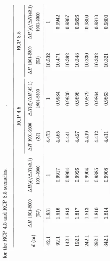
Table Page 1.1 Heat stored in the subsurface since 1901 CE in the year 2000, and

predicted for years 2100, 2200 and 2300 CE for the RCP 4.5 and RCP 8.5 scenarios. . . . . . . . . . . . . . . . . . . .. . . . . . . . 41 1.2 Heat stored in the soil (upper 3.8 rn) since 1901 CE in the year

2000 and predicted for the year 2300 CE for the RCP 4. 5 and RCP 8.5 scenarios. . . . . . . . . . . . . . . . . . . . . . 42 2.1 Areal extent of intermediate-depth permafrost at 1901 CE, 2000

CE and 2300 CE for the RCP 4.5 and RCP 8.5 scenarios. 84 2.2 Areal extent of near-surface permafrost at 1901 CE, 2000 CE and

Figure

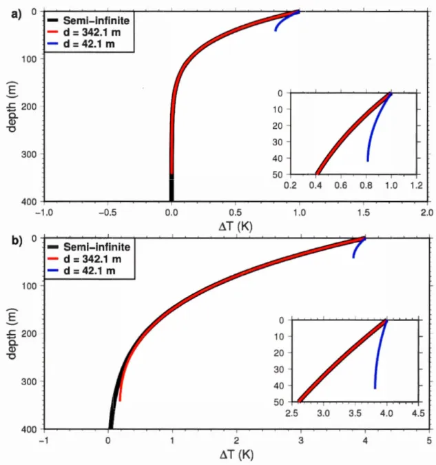
1.01 Departure from the initial temperature profile due to constant rate of surface temperature increase of 0.01 K yr-1

. Analytical solutions for the half space rnodel (black), and for the fini te thickness model with bottom boundary at 42.1 rn (blue) and at 342.1 rn (red). a) Temperature anomal y after 100 yr. b) Temperature anomal y after

Page

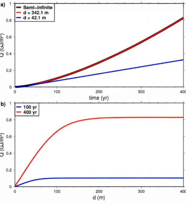
400 yr. . . . . . . . . . . . . . . . . . . . . . . . . . 31 1.02 Heat absorbed by the land column per unit of area (Q), following

the start of a linear surface temperature increase of 0.01 K yr-1_{. a):} Q as a function of time for the half space model and two models of fini te thicknesses 42.1 rn and 342.1 rn. b):

Q as a function of the

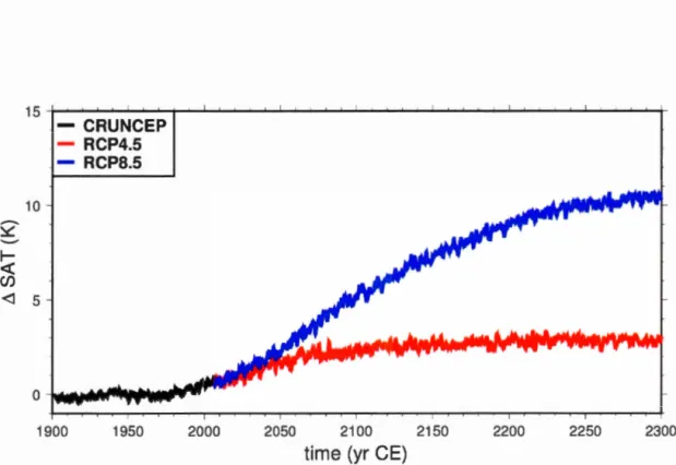
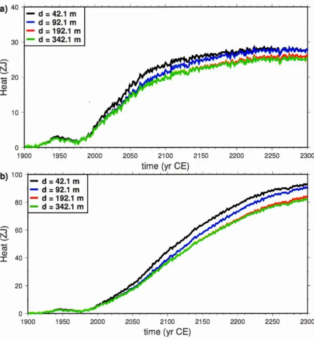
thickness d of the fini te mo del, at 100 yr and 400 yr. . . . . . . . 32 1.03 Mean Surface Air Temperature (SAT) over land relative to the 20th

cent ury mean, from the CRUN CEP dataset (black) and the RCP 4.5 (red) and RCP 8.5 (blue) scenarios. Data taken from Viovy (20r8); Thomson et al. (2011); Riahi et al. (2011). . . . . . . . . 33 1.04 Heat stored in the subsurface as function of time, for models of

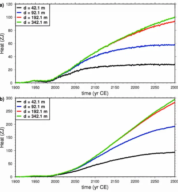
subsurface thickness d of 42.1 rn (black), 92.1 rn (blue) 192.1 rn (red) and 342.1 rn (green). a) Simulations forced with CRUNCEP

+ RCP 4.5 data. b) Simulations forced with CRUNCEP

+ RCP

8.5 data. Note the scale difference between scenarios RCP 4.5 and RCP 8.5. . . . . . . . . . . . . . . . . . . . . . . . . . . . . . 34 1.05 Heat stored in the subsurface as function of subsurface thickness,

at the years 2000 (black), 2100 (blue), 2200 (red) and 2300 (green). a) Simulations forced with CR UN CEP

+

RCP 4.5 data. b) Sim-ulations forced with CRUNCEP

+ RCP 8.5 data. Note the scale

difference between scenarios RCP 4.5 and RCP 8.5. 35

1.06 Heat stored in the upper 42.1 rn as function of time, for models of su bsurface thickness d of 42.1 rn (black) , 92.1 rn (blue) 192.1 rn (red) and 342.1 rn (green). a) Simulations forced with CRUNCEP

+

RCP 4.5 data. b) Simulations forced with CR UN CEP

+ RCP

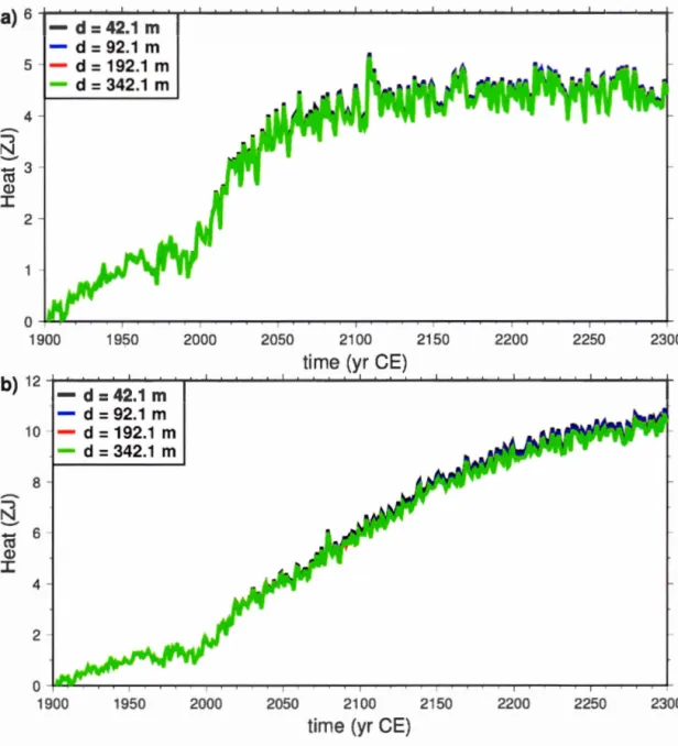
8.5 data. Note the scale difference between scenarios RCP 4.5 and RCP 8.5. . . . . . . . . . . . . . . . . . . . . . . . . . . . . . . 36 1.07 Heat stored in the soil (upper 3.8 rn), for models of subsurface

thickness d of 42.1 rn (black), 92.1 rn (blue) 192.1 rn (red) and 342.1 rn (green). a) Simulations forced with CRUNCEP

+ RCP

4.5 data. b) Simulations forced with CR UN CEP RCP 8.5 data. Note the scale difference between scenarios RCP 4.5 and RCP 8.5. 37 1.08 Heat stored in the sail as function of subsurface thickness, as

frac-tion of that the thinnest madel (d=42.1 rn). Years 2000 (black), 2100 (blue), 2200 (red) and 2300 (green). a) Simulations forced with CR UN CEP -/ RCP 4.5 data. b) Simulations forced with CRUNCEP

+ RCP 8.5

data. . . . . . . . . . . . 38 1.09 Heat stored in the upper 42.1 rn (the thickness of all models is 42.1

rn) as function of crustal heat flux, relative to the initial heat con-tent of the original madel (FB = 0 W m-2). The heat content in each mo del is a static shi ft from th at of the original mo del. a) Sim-ulations forced with CR UN CEP

+ RCP

4.5 data. b) Simulations forced with CRUNCEP

+ RCP 8.5 data.

Note the scale difference between scenarios RCP 4.5 and RCP 8.5.

1.10 Heat stored in the soil (upper 3.8 rn) as function of crustal heat flux, referenced to the initial heat content of the original madel (FB = 0 W m-2

). a) Simulations forced with CRUNCEP

+ RCP

4.5 data. b) Simulations forced with CR UN CEP

+ RCP

8.5 data.

39

Note the scale difference between scenarios RCP 4.5 and RCP 8.5. 40 2.01 Schema of the carbon flux in CLM4.5-BGC. Figure redrawn from

Oleson et al. (2013). . . . . . . . . . . . . . . . . . . . . . . . . . 64 2.02 Region of study (blue), which corresponds to the extent of

near-surface permafrost in the Northern Hemisphere in the year 1901, for the original CLM4.5 madel. . . . . . . . . . . . . . . . 65 2.03 Mean Surface Air Temperature (SAT) over the region of study

rela-tive to the 20th century mean, from the CRUNCEP dataset (black) and the RCP 4.5 (red) and RCP 8.5 (blue) scenarios. . . . . . 66

2.04 Northern Hemisphere intermediate-depth (0-42.1 rn) permafrost area as function of time. Model versions with bottom boundary depth d at 42.1 rn (black), 92.1 rn (blue) 192.1 rn (red) and 342.1 rn (green). a) Simulations forced with CR UN CEP

+

RCP 4.5 data. b) Simulations forced with CR UN CEP

+ RCP 8.5 data. .

. . . . 67 2.05 Northern Hemisphere intermediate-depth permafrost area as

func-tion of subsurface thickness d, at the years 2000 (black), 2100 (blue), 2200 (red) and 2300 (green). a) Sirnulations forced with CR UN CEP

+

RCP 4.5 data. b) Simulations forced with CRUN-CEP

+

RCP 8. 5 data. . . . . . . . . . . . . . . . . . . . . . . 68 2.06 Northern Hemisphere intermediate-depth permafrost area as

func-tion of time. Model versions using different heat flux as bottom boundary. a) Simulations forced with CRUNCEP

+

RCP 4.5 data. b) Simulations forced with CR UN CEP

+

RCP 8.5 data. . . 69 2.07 Northern Hemisphere near-surface permafrost area as function of

time. Model versions with bottom boundary depth at 42.1 rn (black), 92.1 rn (blue) 192.1 rn (red) and 342.1 rn (green). a) Sim-ulations forced with CR UN CEP

+ RCP 4.5 data. b) Simulations

forced with CRUNCEP

+

RCP 8.5 data. . . . . . . . . . . . . . 70 2.08 Northern Hemisphere near-surface permafrost area as function of

time. Models using different heat flux as bottom boundary. a) Sim-ulations forced with CR UN CEP RCP 4.5 data. b) Simulations forced with CRUNCEP

+

RCP 8.5 data. . . . . . . . . 71 2.09 Active Layer Thickness for the unmodified mo del (top)), and

dif-ferences to the original model at each time frame for the modified model with Fs = 80 mW m-2 (middle) and the modified model with d = 342.1 rn (bottom). Time frames at 1901 CE and 2300 CE for the scenarios RCP 4.5 and RCP 8.5. . . . . . . . . . . . 72 2.10 Evolution of soil carbon pool in the Northern Hemisphere

per-mafrost region, compared to the size for the original model at 1901 CE. Models with varying bottom boundary depth. a) Simulations forced with CR UN CEP

+

RCP 4.5 data. b) Simulations forced with CRUNCEP + RCP 8.5 data. Note the different vertical scale in panel a and b. . . . . . . . . . . . . . . . . . . . . . . . 73

2.11 Evolution of soil carbon pool in the Northern Hemisphere per-mafrost region, compared to the size for the original model at 1901 CE. Models with varying basal heat flux. a) Simulations forced with CRUNCEP

+

RCP 4.5 data. b) Simulations forced with CRUN-CEP - RCP 8.5 data. Note different vertical scale in panel a and

b. . . . . . . . . . . . . . . . . . . . . . . . . . . 74 2.12 Distribution of soil carbon for the original model (top) in kgCjm2

, and differences to the original model at each time frame for the modified model with FB

=

0.08 W m-2 (middle) and the modified model with d

=

342.1 rn (bottom), in gCjm2. Time frames at 1901 CE and 2300 CE for the scenarios RCP 4.5 and RCP 8.5. 75 2.13 Mean size of the soil carbon pool in the Northern Hemisphere

per-mafrost region between 1901-1910, as function of basal heat flux. 76 2.14 Vegetation carbon pool in the Northern Hemisphere permafrost

re-gion. Mo dels with varying bot tom boundary depth. b) Simulations forced with CRUNCEP

+

RCP 8.5 data. . . . . . . . . . 77 2.15 Vegetation carbon pool in the Northern Hemisphere permafrost

re-gion. Models with varying basal heat flux. a) Simulations forced with CRUNCEP

+

RCP 4.5 data. b) Simulations forced with CRUNCEP

+

RCP 8.5 data. . . . . . . . . . . . . . . . 78 2.16 Distribution of vegetation carbon for the original mo del (top), and

differences to the original model at each time frame for the modified model with FB = 0.08 W m-2 _{(middle) and the modified model} with d = 342.1 rn (bottom). Time frarnes at 1901 CE and 2300 CE for the scenarios RCP 4.5 and RCP 8.5. . . . . . . . . . . . . . . 79 2.17 Mean size between 1901-1910 of the vegetation carbon pool in the

Northern Hemisphere permafrost region, for models of different bot-tom heat flux. . . . . . . . . . . . . . . . . . . . . . . . . . . 80 2.18 Distribution of methane yearly production for the original model

(top), and differences to the original mo del at each time fr arne for the modified model with FB

=

0.08 W m-2 _{(middle) and the} modified model with d = 342.1 rn (bottom). Time frames at 1901 CE and 2300 CE for the scenarios RCP 4.5 and RCP 8.5. 81

2.19 Global yearly methane production as function of time, moving av-erage of 10 years. Models with varying bottom boundary depth. a) Sirnulations forced with CR UN CEP -\- RCP 4.5 data. b) Simu-lations forced with CRUNCEP -\- RCP 8.5 data. . . . . . . . . . 82 2.20 Global yearly methane production as function of time, moving

av-erage of 10 ye·ars. Models with varying basal heat flux. a) Sim-ulations forced with CR UN CEP -\- RCP 4.5 data. b) Simulations forced with CRUNCEP -1- RCP 8.5 data. . . . . 83 3.01 (a): Vertical temperature profile measured in Dome C. (b):

Con-ductive heat flux profile, calculated from the temperature profile by Fourier law with a temperature-dependent thermal conductiv-ity. Heat flux has been truncated for the upper 225 rn because the temperature profile is very noisy near the surface of the ice sheet. 106 3.02 Sketch of flow in an ice sheet. The velocity of ice particles, both

vertical and horizontal components, is highest near the surface and decreases at depth. The ice motion thins the ice layers and reduces the height of the glacier, while accumulation of snow at the surface increases its height. Temperature in the ice sheet increases clown-ward, as heat flows out of the bedrock, and melting of ice could happen at the base. The ratio of the horizontal components of velocities at the bottom and at the surface of the ice defines the sliding ratio s.

3.03 Variations of thickness in Dome C for the last 800 kyr, simulated with the linear perturbation model developed in Parrenin et al.

107

(2007b). . . . . . . . . . . . . . . . . . . . 108 3.04 Surface accumulation rate his tory (in ice-equivalent units). 109 3.05 Surface Air Temperature (SAT) history.

3.06 (a) Ternperature-depth and (b) heat flux-depth profiles obtained at the end of the sirnulation with different values for the param-eters n and p. Note how shear heating influences the shape of the ternperature and heat flux profiles. The other parameters for these calculations are qb = 49.4 rn W m-2, Vsur = 0.015 rn yr-1, and

110

Toffset = 0 K. . . . . . . . . . . . . . . . . . . . . . . 111

3.07 Histograms of retained values for the free parameters: (a) basal flux, (b) IST-SAT temperature offset, (c) Glen's exponent n, (d) flux function par arne ter p, and ( e) sliding parame ter s. . . . . . . 112

3.08 (a): Temperature-depth profile of Dome C (black) versus a simu-lation using p = 1.8 and s = 0.14 and the most likely values of the other parameters qb = 51.1 mW m-2, n = 1.91 and Toffset = 0.36 K (blue). (b): Conductive heat flux profile determined from the temperature profile, measured at Dome C (black) and calculated for the most likely values (blue). . . . . . . . . . . . . . . . . 113 3.09 (a): Temperature-depth profile and (b) conductive heat flux

pro-file determined from the temperature propro-file, measured at Dome C (black), calculated with artificially made zero shear heating (blue), calculated with shear heating and the theoretical value of the flux shape function parameter p = 9, and calculated with shear heating but p = 2. The values of the other parameters in the simulated profiles aren= 3, s = 0.1, qb = 49.4 mW m-2 and Toffset = 0 K. . 114 2.01 Change in the position of the qb peak, as function of: a) The

temper-ature cutoff Tcutoff, with heat flux cutoff set to qcutoff = 2 rn W m-2,

and b) The heat flux cutoff qcutoff, with temperature cutoff set to Tcutoff

=

Ü. 7 K. . . . . . . . . . . . . . . . . . . . . . . . . . . 128

FB Heat flux used as bottom boundary condition (W m-2_).

H Height of the glacier ( m).

Toffset Temperature offset between the atmosphere the ice surface (K).

n

Rate of heat production per unit volume (J.LW m-3 ).

"" Thermal diffusivity (m2 s-1) .

.À Thermal conductivity (W m-1 _K-1_).

w Flux shape function for the glacier ( unitless).

p Density (kg m-3_).

( Adimensional vertical coordinate for the glacier ( unitless).

a Snow accumulation in ice equivalent units (m y-1 ).

c Volumetrie heat capacity ( J m-3 _K-1 ).

Cp Specifie he at ( J kg-1 K-1).

d Depth of the bottom boundary for the finite thickness model (m).

m Mel ting rate at the bottom of the glacier (rn y-1

).

p Flux function parameter or parameter determining the shear deforrnation com

-ponent of the flux shape function in Lliboutry's approximation ( unitless).

q Conductive heat flow (W m-2 ).

qb Basal heat flux at the bot tom of the glacier (W m-2 ).

s Sliding ratio ( unitless).

t Time coordinate (yr).

ALT Active Layer Thickness.

BGC BioGeoChemistry.

CESM1.2 Community Earth System Model version 1.2.

CLM4.0 Community Land Model version 4.0.

CLM4.5 Community Land Model version 4.5.

CLM5.0 Comrnunity Land Model version 5.0.

CMIP5 Climate Model Intercomparison Project phase 5.

CN Carbon-Nitrogen.

CRU-TS Climate Research Unit Tirne-Series.

ESM Earth System Model.

GST Ground Surface Temperature.

IST lee Surface Temperature. LSM Land Surface Model.

NCEP National Centers for Environmental Prediction.

RCP Representative Concentration Pathway.

La modélisation numérique des processus therrniques souterrains dans les

rnod-èles de surface terrestre nécessite l'utilisation de conditions aux lin1ites inférieures

appropriées pour le sous-sol. Cette thèse est divisée eu trois chapitres: les deux

premiers traitent de la modification des conditions aux limites du sous-sol dans un modèle climatique, afin d'obtenir des profils de ternpérature réalistes et d'étudier leurs conséquences, tandis que le troisième concerne l'application d'un rnodèle

numérique d'un glacier pour obtenir des contraintes d'écoulement glaciaire à

par-tir du profil de ternpérature vertical.

Le premier chapitre exarnine les problèmes découlant de l'utilisation de rnodèles

de surface terrestre avec une linüte inférieure du sous-sol excessivement peu

pro-fondes dans les sirnulations climatiques, ainsi que les effets du flux de chaleur nul

à cette limite inférieure. Une limite inférieure peu profonde reflète l'énergie à la

surface, ce qui, associé à l'absence de gradient géothermique, modifie le bilan

én-ergétique de surface et l'état thermique à long terme du sous-sol. Nous décrivons

le modèle de subsurface dans le Cornmunity Land Model version 4.5 (CLM4.5)

et les rnodifications introduites pour obtenir une limite inférieure suffisamrnent

profonde pour le sous-sol et un flux de chaleur de la croûte non nul à la limite inférieure pour induire un gradient géothermique. Nous opérons les versions mod-ifiées et originales du CLM4.5 entre 1901 et 2300, en utilisant le forçage historique

au cours de la période 1901-2005 et deux scénarios futurs d'émissions modérées

(RCP 4.5) et élevées (RCP 8.5) entre 2005-2300. L'augmentation de l'épaisseur

du sous-sol de 42.1 à 342.1 rn augmente la chaleur stockée dans le sous-sol entre

1901 et 2300 de 217% (RCP 4.5) à 260% (RCP 8.5). En utilisant le flux de chaleur

continental moyen 60 rn W rn -2 â la base du modèle, la température à la frontière

sol-substrat (3.8 rn de profondeur) augmente de 0.12

± 0.03

K et â la base (42.1

rn de profondeur) de 0.8 ± 0.04 K, indépendamrnent du scénario.

En modifiant l'état therrnique du sous-sol et le bilan énergétique de surface, la limite inférieure affecte d'autres éléments du modèle de surface terrestre, tels que le pergélisol, le carbone du sol, la végétation et la production de méthane. Le deuxième chapitre examine comment ces processus sont affectés au cours de la période 1901-2300 dans les mêmes simulations que celles décrites dans le deuxième

chapitre. L'augmentation de l'épaisseur du sous-sol de 42.1 à 342.1 rn réduit de

1901 et 2300, et réduit la perte de carbone dans le sol de 1.6% (RCP 4.5) à 3.6% (RCP 8.5). Un flux de chaleur crustal de 80 n1W m-2 _{a peu d'effet sur l'étendue} du pergélisol, rnais il réduit la perte de carbone dans le sol de 4.4% (RCP 4.5) à

22.4% (RCP 8.5). Ces effets sont non négligeabl s, ce qui suggère que l'utilisation de conditions de base appropriées pour le sous-sol est nécessaire pour obtenir une représentation robuste, non seulernent du régirne therrnique terrestre, rnais aussi des processus se produisant dans la surface et le sous-sol peu profond.

Le troisièrne chapitre présente un rnodèle nurnérique de l'écoulement vertical de la glace et de la génération et de la conduction de la chaleur dans un glacier.

Il est appliqué au profil de température rnesuré dans le forage à EPICA Dame C dans l'Antarctique de l'Est. Ce modèle utilise l'histoire de la température de l'air en surface, de l'accumulation de neige et de la hauteur du glacier en tant que conditions limites et calcule le profil vertical actuel de la température, qui dépend de plusieurs paramètres (inconnus) de l'écoulement glaciaire. Nous util-isons la rnéthode de Monte-Carlo pour obtenir des contraintes sur ces paramètres: nous explorons l'espace des parametres et comparons les profils de ternpérature calculés avec le profil mesuré pour trouver des distributions de probabilités pour les paramètres inconnus. Nous avons déterrniné un flux de chaleur de la croûte de 51.1

±

1.4(2(}) n1W m-2

, supérieur à la valeur apparente (rnesurée directement

à la base du glacier). Nous avons trouvé une valeur pour l'exposant de Glen de 1.91

± 0

.11(2(}) et un couplage de température air-glace de 0.36 ± 1.2(2(}) K. Le rapport de glissernent est limité à une valeur rnaximale de 0.4 et le paramètre de la fonction flux à une valeur maximale de 7.4, avec un intervalle de confi-ance 2(}. Notre rnodèle est capable d'obtenir de valeurs bien contraintes pour les pararnètres les plus irnportants de l'écoulernent de la glace. Le modèle peut être appliqué à d'autres sites, mais les résultats peuvent être affectés par des valeurs élevées de fusion à la base du glacier.

Mots clés: Modèles climatiques, rnodèles de surface terrestre, flux. thermique, températures souterraines, limite inférieure, gradient géothermique.

Numerical modelling of subsurface therrnal processes in land surface models re-quires the use of appropriate bottom boundary conditions for the subsurface. This thesis is divided in three chapters: the first two deal with the modification of the land subsurface boundaries in a climate model to obtain realistic temperature profiles and a study of its consequences, while the last concerns the application of a numerical model of a glacier to obtain constraints of glacier flow from the vertical temperature profile.

The first chapter examines the problems that arise from the use of land surface models with too-shallow subsurface bottom boundaries in climate simulations and

also the effect of zero heat flux at such bottom boundary. Shallow bottom

bound-aries reflect energy to the surface, which along with the lack of a geothermal

gradient, alters the surface energy balance and the long-term thermal state of the

subsurface. We describe the subsurface model in the Community Land Model

version 4.5 (CLM4.5) and the modifications introduced to obtain a sufficiently deep bottom boundary for the subsurface and a non-zero crustal heat flux added

at the bottom boundary to induce a geothermal gradient. We run the modified

and original CLM4.5 between 1901 and 2300, using historical forcing during the period 1901-2005 and two future scenarios of moderate (RCP 4.5) and high (RCP 8.5) emissions between 2005-2300. Increasing the thickness of the subsurface from

42.1 rn to 342.1 rn increases the heat stored in the subsurface between 1901 and

2300 by 217% (RCP 4.5) to 260% (RCP 8.5). Using the mean continental heat flux 60 rn W m-2 at the bot tom of the model rises the temperature at the soil-bedrock frontier (3.8 rn depth) by 0.12

±

0.03 K and the bottom of the model

( 42.1 rn depth) by 0.8 ± 0.04 K, independently of the scenario.

By altering the thermal state of the subsurface and the surface energy balance,

the bottom boundary affects other elements of the land surface model such

asper-mafrost, soil carbon, vegetation, and methane production. The second chapter

investigates how these processes are affected during the period 1901-2300 in the

same simulations as those described in the second chapter. Increasing the

thick-ness of the subsurface from 42.1 rn to 342.1 rn reduces the loss of near-surface

permafrost between 1901 and 2300 by 1.6% (RCP 4.5) to 1.9% (RCP 8.5), and

reduces the loss of soil carbon by 1.3% (RCP 4.5) to 3.6% (RCP 8.5). A crustal

the loss of soil carbon by 4.4% (RCP 4.5) to 22.4% (RCP 8.5). In the local scale these differences can be one arder of magnitude with respect to the original madel. These effects are non-negligible, which suggests that the use appropriate bottom boundary conditions for the subsurface is necessary to obtain a robust represen-tation, not only of the land thermal regime, but also of the processes taking place in the surface and the shallow subsurface.

The third chapter introduces a numerical rnodel of vertical ice flow and the gener-ation and conduction of heat in a glacier. It is applied to the temperature profile measured at EPICA Dome C in East Antarctica. This madel uses histories of surface air temperature, snow accumulation and glacier height as boundary con-ditions, and calculates the present vertical profile of temperature, which is depen-dent on sever al ( unknown) parameters of glacier flow. We use the Monte-Carlo method to obtain constraints on these parameters, we compare the calculated temperature profiles with the measured profile and explore the parameter space to find probability distributions for the unknown parameters. We determi~ed a basal heat flux 51.1±1.4(2a) mW m-2

, higher than the apparent value (measured directly at the base of the glacier). We found a value for the Glen's exponent of 1.91+0.11(2a) and an air-ice temperature coupling of0.36±1.2(2a) K. The sliding ratio is constrained to a maximum value of 0.4 and the flux function parameter to a maxirnum value of 7.4, with a 2a confidence interval. Our madel is able to obtain well constrained values for the most important parameters of ice flow. The model can be applied to other sites, but the results of the Monte-Carlo method can be affected by high values of melting at the base of glacier.

Keywords: Climate rnodels, land surface models, heat flow, subsurface tempera-tures, bottom boundary, geothermal gradient.

The numerical modeling of the climatic system is a valuable tool for scientists to understand climate. Clirnatic mociels are used for a variety of purposes, from studying the dynamics of the climate system to weather forecast. One of the most common applications of climate models is the study of climate change and the investigation of the impacts of the perturbations caused by human activities. Projections of future climate are based on ensembles of Earth System Models (ES Ms), large numerical mo dels including the different subsystems of Earth's climate, the oceans, the atmosphere, the land, the cryosphere and the biosphere, coupled together (Stocker et al., 2013).

Modeling of climate is a difficult task, as the natural processes that influence Earth's climate are numerous and complex. Clirnate modelers have been histor-ically been limited by their capacity to understand and rnodel these processes, as well as by the computational resources available to them. Starting from the relatively simple early climate models (Phillips, 1956), ESMs have improved in-crementally, building on previous generations of ESMs as the understanding of climatic processes and our computational capabilities kept improving (McGuffie

& Henderson-Sellers, 2001). Because of the large scope of this task, modelers prioritize their efforts on the processes they consider most important for a model, which means the modeling of sorne natural processes can be temporally neglected in favor of others.

While the circulation of the atmosphere and the oceanic currents are the main drivers of Earth's climate, the land system plays an important role in it through

the interactions between the land and the atmospheric and oceanic circulation.

For instance, the land's vegetation stores atmospheric carbon, which over time

be-cornes part of the soil carbon pools (Scharlemann et al., 2014), soil color type and

snow cover play important roles in the surface's energy budget through the albedo

(Hansen & Nazarenko, 2004), and the land hydrology also affects the ocean's

ther-mohaline circulation through river freshwater discharge (Bray, 1988). Therefore, the mo dels of the land system or Land Surface Mo dels (LSMs) have evolved to provide more precise descriptions of the surface energy balance (Pitman, 2003; Hansen & Nazarenko, 2004), the surface water balance (Seneviratne et al., 2010), vegetation and land use (Bonan, 2008), and carbon dynamics (Ramanathan &

Carmichael, 2008).

When this thesis was started, the latest generation of LSMs was integrated in the ESMs that formed part of the Climate Model Intercomparison Project phase

5 (CMIP5) (Taylor et al., 2012). These LSMs include more complex and more

complete descriptions of natural processes than the previous generation of LSMs,

specially for carbon dynamics, vegetation and land use ( Oleson et al., 2013; Best

et al., 2011; Ji et al., 2014; Friend & Kiang, 2005; Schmidt et al., 2014; Weaver

et al., 2001). However, there are important limitations in the modeling of the

subsurface across these models. Among several simplifications, such as an homo

-geneus and unrealistically shallow regolith thickness or an hydrology restricted to

the soil, most of these models lack a geothermal gradient and use an excessively

shallow bottorn boundary for the subsurface (Cuesta-Valera et al., 2016).

The main justification to exclude the geothermal gradient and restrict the

sub-surface model to the upper subsurface is that, in the short time scale, the deep

subsurface does not interact with climate. Most LSMs place the bottom

bound-ary of the subsurface at a depth of 3-4 rn, which is considered adequate for basic hydrology calculations, root uptake and carbon dynarnics (Cuesta-Valero et al.,

2016). At such depth, the effect of the geothermal gradient (with a global average value of r-v 0.02K/m (Jau part & Mareschal, 2015)) is very small, and it is th us ignored in the LSMs. However, this depth is too shallow to pro perl y mo del the long-term thermal behavior of the subsurface (MacDougall et al., 2008, 2010).

The dynamics for the propagation into the subsurface of long trends of tempera-ture at the surface of the land system are well known (Carslaw & Jaeger, 1959). As a periodic thermal signal propagates into the subsurface, it is attenuated ex-ponentially in depth, with a skin depth proportional to the square root of the period of the signal. Similarly, the time that a periodic thermal signal from the surface takes to reach a given depth is proportional to the square of this depth (Lesperance et al., 2010). This relationship allows borehole climatology to use the thermal profiles of the subsurface to reconstruct the past Ground Surface Tem-perature ( GST) history. The reconstruction of long GST histories requires deep boreholes: boreholes of few hundred meters are only used to reconstruct events more recent th an 500 yr, and boreholes of r-v 1500 rn are used to reconstruct elima te variations on the scale of 10 to 100 kyr (Pickler et al., 2016).

This relationship between the depth reached by a thermal signal and the time that it takes for the signal to reach such depth is at the root of our concerns. State of the art ESMs in the CMIP5 are currently used to project future climate change during the next 100 to 300 yr (Stocker et al., 2013). However, the LSMs used in these ESMs place the bottom boundary at depths of 3.5 to 10 rn (Cuesta-Valera et al., 2016), with one exception of 42.1 rn (Oleson et al., 2013). Such depths are much smaller than those reached by centennial trends of surface temperature. As the bottom boundary in LSMs uses a constant heat flux, it acts like a barrier for the propagation of heat, and therefore an insu:fficient depth affects the propaga-tion of thermal signals underground. This has been shown in theoretical estimates of the heat stored by the subsurface during a ESM simulation of the 21st century

show a one order of magnitude difference between models using subsurface thick-nesses of 10 rn and 600 rn (MacDougall et al., 2008). Not only does this severely ·

underestimate the amount of heat absorbed by the subsurface, but as the thermal

signal is unable to propagate past the bottom boundary, it is reflected upwards,

thus creating a disturbance in the portion of the subsurface that is being

simu-lated. To avoid reflected heat signals to affect the thermal profiles, the bottom boundary of the LSMs used in ESMs must be suffi.ciently deep for the duration of

the simulations.

As the lack of geothermal gradient and the insufficient depth of the bottom bound-ary perturb the thermal profiles of the subsurface, they will also affect other

sub-systems of a LSM that are dependent on the temperature of the subsurface. In

particular, the carbon dynamics could be significantly affected. The methabolic rates of the microorganisms that intervene in the decay of organic matter or in the production of methane are sensitive to temperature, which creates a feedback between the activity of these microorganisms in the land system, and the green-house gas concentrations and temperatures in the atrnospheric system (Heimann

& Reichstein, 2008). In addition, because a LSM of insufficient subsurface thick-ness overestimates the speed at which the upper subsurface adapts to variations

in atmospheric temperatures, it also underestimates the stability of perrnafrost.

Changes in extension or depth of permafrost in a LSM has further repercussions

in hydrology and microbial activity.

The geothermal gradient and an adequate depth of the bottom boundary are

therefore two key elements, necessary for modeling the land thermal regime, that

are absent in current LSMs. Their impact can be estimated analytically in terms

of heat absorption by the subsurface (Stevens et al., 2007), but to know their effect on other subsystems of the land rnodel requires to use numerical simulations.

The main objective of this thesis is to deterrnine and analyze the effect of a too shallow bottom boundary and a nul geothermal gradient in a LSM. With this, we airn to convince modelers of the significance of these two limitations,

and lead them to overcome these limitations in future LSMs. While the lack of geothermal gradient and an excessively shallow subsurface are far from being the only limitations of current LSMs, we have to limit the scope of our project, because of the limited time and resources available to us. In the sarne way as LSMs are improved incrementally, expanding and developing the different parts of a model one step at a time, we have focused on the improvernent of the land thermal regirne.

This thesis is presented as three different chapters in the form of three scientific

articles. The three articles share a comrnon theme: the use of numerical models to

study the propagation of long trends of air surface temperature into the subsurface,

and how the resulting temperature-depth profiles depend on the characteristics of

the su bsurface mo del.

The first and second chapters of this thesis correspond to one scientific article that was originally planned to be published in two parts, but that was finally submitted as one single paper. This article has been accepted for publication in Geoscientific Model Development, under the title «Lower boundary conditions in Land Surface

Models. Effects on the permafrost and the carbon pools: a case study with CLM

4.5», and as for March 2019 it is in discussion phase. In these two chapters we develop the main subject of the thesis, analyzing the effect of excessively shallow bottom boundaries and lack of geothermal gradient in LSMs. To that end, we

modify the Community Land Model version 4.5 (CLM4.5) (Oleson et al., 2013).

We create new versions of this model by either increasing the depth of the bottom

boundary or by using different values of bottom heat flux. To compare these

different versions are subject to the same set of atmospheric forcings (temperature,

precipitation, solar radiation, winds and atmospheric pressure).

In the first chapter, we develop the theoretical framewor k for the propagation

of surface thermal signals into the subsurface, and the relationship between the

time scale of the surface signals and the depth at which they propagate, from

where we obtain estimates of how the depth of the bottom boundary affects the

propagation of heat underground. We describe the subsurface madel in CLM4.5

and explain how we modify the mo del to increase to depth of the bot tom boundary

and to change the basal heat flux. We also provide a cornplete description of the

numerical experiments and the set of atmospheric data used to force the CLM4.5

during the simulations. Finally, we analyze the propagation of the surface thermal

signal into the subsurface for the different versions of the CLM4.5.

In the second chapter, we expand the numerical simulations described in the first

chapter, to investigate the effects of the geothermal gradient and the thickness

of the subsurface on several elements of the madel: depth and areal extent of

permafrost, the soil carbon pool, the vegetation, and the production of methane.

These effects are analyzed at two spatial scales: at the local scale of the land cells

defined by the spatial discretization of the numerical madel, and at the regional

scale of the Northern Hemisphere permafrost region.

Finally, the third chapter of this thesis corresponds to one article we developed

to make use of a thermal profile measured from the ice core at the EPICA Dome

C site in East Antarctica in 2004 (Augustin et al., 2004). In this chapter, we

developed a numerical method to introduce constraints on several key parameters

of glacier flow, using the present thermal profile of the glacier and geode tic data.

This article was submitted to the scientific journal Clirnate of the Past, but was

Decem-ber 12, 2016), who collected and provided us the data used in the article. An unfortunate miscommunication caused us to believe that we had permission to

use this data, which was not the case. Catherine Ritz agreed to the inclusion of

this paper in this thesis.

The analysis of ice cores provide reliable records of past climate, going back hun-dreds of thousands of years into the past (Parrenin et al., 2007a; Jouzel et al., 2007). The analysis of the air bubbles trapped in the ice allows the reconstruc-tion of the past concentrations of atmospheric gases such as C02 , CH4 and N20

(Barnola et al., 1987; Spahni et al., 2005). The ice cores also allow to reconstruct

the history of past atmospheric temperatures and past accumulation rates, from

the analysis of stable oxygen isotope ratios and deuterium in the ice core (Jouzel

et al., 2007; Pol et al., 2010). The ice core at Dome C, drilled by the European

Project for lee Coring in Antarctica (EPICA), provides these records for the past 800 kyr, which makes it one of the longest records currently available (Augustin

et al., 2004).

In addition to past atmospheric composition, atmospheric temperature and snow

accumulation, the measurement of the ice temperature in the ice core provides a

high resolution temperature-depth profile of the ice sheet. These thermal profiles are used to calculate the conductive heat flux, which allows the estimate the crustal heat flux at the measurement site (Fisher et al., 2015). However, this

estimate is a first order approximation, because there are more factors affecting

the thermal profile other than the crustal heat flux. First, the thermal profile is

affected by the past history of atmospheric temperatures at the top of the glacier,

as this thermal signal propagate downwards. Second, the deformation of the ice

pro duces internai heating, rising temperature inside the glacier. To determine the

In land, the relationship between the history of past ground surface tempera-tures and the present temperature-depth profiles is the base of borehole paleo-climatology (Mareschal & Beltrarni, 1992). Because the thermal regime of the continental deep subsurface is purely conductive, inverse rnethods can be applied to reconstruct past ground surface temperatures from the temperature-depth pro-file (Jaupart & Mareschal, 2010). However, these analytical methods can not be applied to isolate the contributions of the surface temperature history and the crustal heat flux in glaciers, because the thermal regime of the glacier is not con-ductive due to the flow of the ice. Instead, we used a numerical rnodel to simulate the flow of ice and the thermal dynamics of the glacier at Do me C.

We developed a one-dimensional numerical model to simulate the glacier at Dome C, which includes the flow of ice and the generation and conduction of heat. This mo del simula tes the past 800 kyr using as boundary con di ti ons the reconstructed histories of past atmospheric surface temperatures, snow accumulation and glacier height at Dome C, obtained from the analysis of Deuterium content in the ice core and from a 1-D ice flow mo del at Do me C ( J ouzel, 2007; Parrenin et al., 2007b).

In Dome C, in addition the crustal heat flux, we find several parameters of ice flow th at are undetermined. We use a Monte-Carlo method to determine the unknown parameters at Dome C, by randomly sarnpling their values. The numerical model yields a thermal profile at present, which is determined by the values of these parameters. By comparing the calculated thermal profile to that measured at Dome C, we obtain a 'goodness of fit' measurement (how close the profiles are) for a specifie location in the parameter space. In this way, we are able to deterrnine a probability distribution for the unknown parameters, their most likely values and the range of acceptable values.

My contribution to these articles constitutes the principal part of each article. In the first and second chapters, I modified the CLM4.5, tested and perforrned simu-lations, and analyzed and interpreted the results. In the third chapter, I developed and tested the numerical madel and analyzed the results. My thesis director, Dr. Hugo Beltrarni, and my thesis codirector, Dr. Jean-Claude Mareschal, developed the theoretical framework for the first and second chapters, provided the ideas for the third chapter, and helped with the editing of the three manuscripts. Dr. Mareschal also participated in the development of the theoretical development needed for the third chapter. The first and second articles are cosigned by Dr. Andrew H. MacDougall, who provided his expertise for the analysis of the results, and made many useful comments while writing the papers.

LOWER BOUNDARY CONDITIONS IN LAND SURFACE MODELS. PART 1: HEAT STORAGE AND TEMPERATURE-DEPTH PROFILES.

1.1 Abstract

Earth System Mo dels (ES Ms) use bot tom boundaries for their land surface mo del components which are shallower than the depth reached by surface temperature

changes in the centennial time scale associated with recent climate change.

Shal-low bottom boundaries reflect energy to the surface, which along with the lack

of geothermal heat flux in current land surface models, alter the surface energy

balance and therefore affect sorne feedback processes between the ground surface

and the atmosphere, such as permafrost and soil carbon stability. To estimate

these impacts, we modified the subsurface model in the Community Land Model version 4.5 (CLM4.5) by setting a non-zero crustal heat flux bottom boundary condition and by increasing the depth of the lower boundary from 42.1 rn to 342.1 m. The modified and original land models were run during the period 1901-2005 under the historical forcing and between 2005-2300 under two future scenarios

of moderate (RCP 4.5) and high (RCP 8.5) emissions. Increasing the thickness

of the su bsurface by 300 rn increases the he at stored in the su bsurface by 72 ZJ

(1 ZJ = 1021 _{J) by year 2300 for the RCP 4.5 scenario and 201 ZJ for the RCP 8.5}

scenario (respective increases of 260% and 217% relative to the shallow model),

the mean continental heat flux 0.06 W m-2 at the bottom of the model rises the temperature at 3.8 rn (the soil-bedrock interface) by 0.12±0.03 K and the bottom bedrock layer by 0.8 ± 0.04 K, independently of the scenario. We determine the optimal subsurface thickness to be 100 rn for a 100 yr simulation and 200 rn for a simulation of 400 yr.

1.2 Introduction

In the current context of anthropogenic climate change, there is a need to forecast future impacts of climate change as accurately and reliably as possible. Future climate change projections are based on simulations from ensembles of Earth System Mo dels (ES Ms), numerical mo dels of oceans, atmosphere, land, ice, and biosphere subsystems coupled together (Stocker et al., 2013). Modeling of the land system has rnainly focused on the interactions between the land surface and the atmosphere (Pitman, 2003), including biogeochemical cycles taking place in the shallow subsurface or soil, such as carbon dynamics (Rarnanathan & Carmichael, 2008), soil moisture (Seneviratne et al., 2010), vegetation cover and land use (Bonan, 2008), and surface processes such as albedo and snow cover (Hansen & Nazarenko, 2004). The bedrock layer present below soil is impermeable, and when explicitly rnodeled, the only process taking place in bedrock is thermal diffusion.

Thermal diffusion in the subsurface allows the land system to act like a heat reservoir, contributing to the thermal inertia of Earth's climate. However, this contribution is relatively small as the capacity of the oceans to absorb energy is orders of magnitude ab ove th at of the continents (Stocker et al., 2013). Estima tes of the energy accumulation during the second half of the 20th century in the land systern show that the heat stored in continents (9 ± 1 ZJ, where 1 ZJ

=

(1021 J) is less th an the uncertainty on the he at stored in oceans d uring the same period (240 ± 19 ZJ (Beltrami et al., 2002; Levitus et al., 2012; Rhein et al., 2013)).

This allows many ESMs to only consider the land subsurface to the shallow depth

(3 - 4 rn) needed for soil modeling (Schmidt et al., 2014; Wu et al., 2014) and

neglect the bedrock entirely. Still, the thermal regime of the subsurface affects

the energy balance at the surface, which in turn influences the surface and soil

processes with a feedback on the clirnate system. Energy variations at the land

surface propagate underground, and the use of a too shallow subsurface in land

models implies that these signals are reflected towards the surface, altering its

energy balance (Smerdon & Stieglitz, 200.6; Stevens et al., 2007).

Sever al works (MacDougall et al., 2008, 2010) have pointed out that, for the long time scales of climate change, the temperature variations at the land surface propagate much deeper than the depths considered in current land models, which range between rv 3.5 rn (Schmidt et al., 2014; Wu et al., 2014) and 42 rn (Oleson

et al., 2013). Theoretical estima tes (MacDougall et al., 2008) of he at stored by

the subsurface show a difference of one order of magnitude between models using

subsurface thicknesses of 10 rn and 600 m. This suggests that the reflected

en-ergy in shallow land models affects the surface energy balance in the simulations,

and current ESMs should use land models sufficiently deep for the length of the

simulations, to avoid bottom boundary effects on the thermal profiles.

Most of the current land models use a zero heat flux as thermal boundary condition at their base, as the geothermal gradient is small ( rv 0.02 K/m) and does not affect

temperature much at shallow depth (Jaupart & Mareschal, 2010). Subsurface

models that increase the depth of the bottom boundary to hundreds of meters

have to consider the geothermal gradient to properly represent the thermal regime of the subsurface. This can be easily irnplemented by using the Earth's crustal heat flux as bot tom boundary condition of the land model, as a few models already

Soils in permafrost regions act as a long-term carbon sink that stores an estimate of 1100-1500 GtC of organic carbon, twice the carbon content of the pre-industrial atmosphere (MacDougall & Beltrami, 2017; Hugelius et al., 2014). The feedback between climate and permafrost thawing and associated carbon emissions is ex-pected to accelerate global warming (Schuur et al., 2015). Rising temperatures at high latitudes induce the thawing of permafrost, leading to the decay of frozen organic matter and the release of C02 and CH4 into the atmosphere. We expect that, both the thickness of the subsurface and setting a realistic non-zero value of heat flux as bottom boundary condition will affect the evolution of permafrost in a warming scenario, and therefore the release of permafrost carbon.

It is possible to use analytical methods to estirnate the effect that the depth of the bottom boundary and the use of a non zero basal heat flux as bottom boundary condition have on the thermal profile of the ground (Stevens et al., 2007). Because of the complexity of the biogeochemical pro cesses in the soil, only numerical simulations can estimate how these processes are affected by the · changes in the thermal profiles. In this paper, we study the effect of the increase of the lower boundary depth and the addition of a geothermal heat flux at the base of the Community Land Model version 4.5 (CLM4.5) (Oleson et al., 2013), which is the deepest ( 42.1 rn) of the current land mo dels used in the Climate Mo del Intercomparison Project phase 5 ( CMIP5) (Stocker et al., 2013). We carried out simulations between 1901 CE and 2300 CE, using historical clirnate reconstruction between 1901 and 2005 (Viovy, 2018) and explored two alternative scenarios of mo derate and high radiative forcings between 2006 and 2300 (Thomson et al., 2011; Riahi et al., 2011).

1.3 Theoretical analysis

The Earth's continental lithosphere (> 100 km) can be considered as a

semi-infinite solid for the centennial and millennial time scales considered in the future projection of climate. For a purely-conductive thermal regime of the subsurface, the propagation of a temperature signal at the surface into the ground is governed

by the heat diffusion equation in one dimension (Carslaw & Jaeger, 1959):

8T 82_T

8t

= re 8z2 ' (1.1)

where re is thermal diffusivity. The solution of Eq. (1.1) for a step change T0 in

surface temperature at t = 0 yields the temperature anomaly at depth z and at time t:

T(

z,

t)

=

T0

e

rfcC~).

(1.2)

The general solution for any surface temperature perturbation T0(t) starting at t

=

0 can be obtained as the convolution in time of T0(t) and the Green function

associated to Eq. (1.1) and the boundary conditions. As the Green function is the solution to a Dirac's delta, it is obtained as the general solution is the time derivative of the solution to the step function in Eq. (1.2). Therefore, the general solution is: - z - 3/2 z

1

t ( 2 ) T(z, t) -

2

~ 0 T0(Ç)(t- Ç) exp -4re(t _ Ç) dÇ. (1.3)

Future scenarios (Van Vuuren et al., 2011) predict rising atmospheric temperatures during the present cent ury ( Cubasch et al., 2013) with a wide mar gin of variability and uncertainty. We can represent this future rise of temperatures by a linearly increasing surface temperature T0(t) = mt, with m being the rate of temperature

increase. For such surface temperature function, the solution to Eq. (1.1) is:

T(

z,

t)

=

mt[(1+

₂

z

~t)

e

rf

c

C~)- ~

exp(~::)].

_(1.4)

Numerical rnodels, however, cannot simulate the subsurface as a semi-infinite solid,

also known as half space model, but instead limit the subsurface to a given depth,

that varies between models. Many land rnodels include only the upper 3 - 4 rn of

the subsurface, which they consider as soil, to model the most basic hydrological processes such as infiltration and runoff in a first-order approximation. Other models further extend the subsurface to include the bedrock below, the deepest

currently being the CLM4.5 with a total depth of 42.1 m. We can simplify these

models by considering conduction only and modeling the land subsurface as a

solid bounded by two parallel planes. Assuming a lower boundary condition of no

heat flux (as most current models do) and a temperature increasing linearly with time T₀(t) = mt as surface boundary condition, we obtain the following solution to Equation (1.1) (Carslaw & Jaeger, 1959):

T(z,t)

=m

~(-l)n

{

(t

+

(

2

n~:z)

2

)

erfc

c~~z)

- (2nd+z)

(:Kr

xp (

_(2n!~z?)

+

+

(t

+

(2(n

+

~~d-

z)2) erfc ( (2(n

;~-

z)) _

-(2(n

+

l)d- z)

(:Kr

exp (-(2(n

\~:-

z)

2)} ,

(1.5) where d is the depth of the bot tom boundary. N eglecting near-surface pro cesses

such as hydrology or snow isolation, the temperature of the subsurface is described

by Eq. (1.5).

Using Eqs. (1.4) and (1.5), we can estima te the effect of the thickness of the

model. We have calculated the profiles of temperature perturbation for a rate

of surface temperature increase of 0.01 K yr-1

, assuming a thermal diffusivity of

K, = 1.5 x 10-6 m2 s-1 (used for bedrock in the CLM4.5 (Oleson et al., 2013)).

This temperature increase is within the range of global temperature projections for the 21st century (Collins et al., 2013).

We calculated the temperature anomalies for the half space madel and the layers of thickness 42.1 rn and 342.1 rn, after 100 yr and 400 yr. After 100 yr the temperature anomaly for the thinnest ( 42.1m) rnodel has departed from that of the half space madel (Fig. 1.01a), while the thickest (342.1 rn) madel cannat be distinguished frorn the half space solution after 100 yr. After 400 yr the thickest madel only has small departure near the base (Fig. 1.01b). The response of a madel of finite thickness approaches that of the half space madel, as long as the bottom boundary is deep enough for the difference between Eqs. (1.4) and (1.5) to be negligible.

The maximum time before the shallow bottom boundary affects the thermal be-havior of the madel is better appreciated in terms of heat absorption by the subsurface. The heat stored in the subsurface can be calculated from the tem-perature change in Eq. (1.5) by assuming a uniform volumetrie heat capacity c

= 2 x 106 _{J m-}3 _K-1 _{(value used for bedrock in the CLM4.5).}

The heat absorbed per unit of area for the 42.1 rn madel is slightly smaller than that of the half space madel after 100 yr and less than half after 400 yr, while for the 342.1 rn madel no difference can be observed (Fig. 1.02a). The heat absorbed after 100 yr or 400 yr increases with the thickness of the rnodel, but reaches a plateau where further increase in thickness does not affect heat storage (Fig. 1.02b). A bot tom boundary depth of 342.1 rn is enough for a simulation lasting 400 yr, but a bottom boundary depth of 42.1 rn is not adequate for a simulation of 100 yr. A bottom boundary depth d = 100 rn is enough for a simulation of 100 yr, as the heat absorbed by the land column does not increase much with further increasing d. A sirnulation of 400 yr, 4 times longer, needs a bot tom boundary depth of d = 200 rn, only twice as mu ch (Fig. 1.02b).

The heat equation (1.1) shows a scaling relationship between bottom boundary

depth d and time t, da

v;:t.

This relation can be used as a first order estimate of the depth where the lower boundary does not affect the therrnal profiles for a given duration of the simulation and a value of diffusivity K-.

1.3.1 Geothermal gradient

In the conductive regime described by Eq. (1.1), the subsurface temperature at a depth z is given as a combination of the geothermal temperature gradient and the temperature perturbation Tt induced by a time-varying temperature signal at the surface:

z

T(z, t) = Ta + qa~

+

Tt(z, t), (1.6)

where Ta is the the mean surface temperature, qa is the geothermal heat flux and

z /À is the thermal depth and À is the thermal conductivity of the subsurface.

The propagation into the subsurface of an harmonie temperature signal such as the annual air temperature cycle is characterized by exponential amplitude atten-uation exp( - j f iz) (Carslaw & Jaeger, 1959), where w is the frequency of the signal and K- is the thermal diffusivity. At depths of 3- 4 m, the amplitude of the

annual signal is sever al degrees. Given the small values ( ~ 0.02 K m-1

) of the geothermal temperature gradient in the continents (Jaupart & Mareschal, 2010), the temperature near the surface is dominated by the surface signal Tt. Therefore

it may seem reasonable to neglect the geothermal gradient for a thin subsurface layer used in land models (Schmidt et al., 2014; Wu et al., 2014). However, the geothermal temperature gradient can still be infiuential, even at shallow depths, for temperature-sensitive regimes of subsurface such as permafrost, and it is nec-essary to determine the lower limit of permafrost. In the case of the CLM4.5 with a subsurface thickness of 42.1 m, the temperature at the bottom of the model is increased by ~ 0.8 K by a geothermal gradient of 0.02 K m-1

. If we were to further increase the thickness of the subsurface, the temperature at the bottom

of the model would increase proportionally.

1.4 Methodology

1.4.1 Original Land Model

The Community Earth System Model version 1.2 (CESM1.2) is a coupled ESM, consisting of components representing the atmosphere, land, ocean, sea-ice and land-ice. Individual components can be run separately, taking the necessary inputs from prescribed datasets. Because running the coupled model is computationally

expensive, we have run only the land model CLM4.5 (Oleson et al., 2013), forced

with prescribed atmospheric inputs (Viovy (2018); Thomson et al. (2011); Riahi

et al. (2011), see section 1.4.3). These inputs are precipitation, solar radiation,

wind speed, surface pressure, surface specifie humidity, Surface Air Temperature

(SAT) and atmospheric concentrations of aerosols and C02 .

Carbon and nitrogen cycles are included in the CLM4.5 through the BioGeo-Chemistry (BGC) module, which includes a methane module (Riley et al., 2011). CLM4.5-BGC can be run at several spatial resolutions. We have used the inter-mediate resolution 1.89°lat x 2.5°lon that allows us to compromise between grid fineness and computational requirements. We used the default timestep of 30 rninutes (Kluzek, 2013).

The subsurface is discretized in 15 horizontallayers with exponentially increasing

node depths:

where fs = 0.025 rn is the scaling factor. Layer thickness ~zi is:

0.5(z1

+

z2) i = 1

~Zi

=

0.5(zi+1 - Zi-1) i = 2 ... 14 (1.8) i = 15

The total thickness of the model is 42.1 m. The upper 10 layers, to a depth of 3.8

rn, are soillayers where biogeochemistry and hydraulic processes take place. The

lower 5 layers are the bedrock, where the only process is thermal diffusion. The

soil in each land column has a vertically-uniform clay /sand/silt composition and

a vertically-variable carbon density (where most of the carbon is concentrated in the upper layers and its concentration decreases with depth), which deterrnines its hydraulic properties and, along with its time-varying water content, its thermal properties. Bedrock layers, assumed to be rnade of saturated granite ( without pores or interstices th at could absorb water), are uniform both horizontal and vertically. The thermal properties for bedrock in CLM4.5 are a thermal conduc-tivity À

=

3 W m-1 K-1 and a volumetrie heat capacity c = 2 x 106 _{J m-}3 _K-1,

which give a thermal diffusivity K = Àjc = 1.5 x 10-6 _{m 2 s-}1 (Oleson et al., _2013). As the horizontal dimensions of the grid are much larger than the thickness of

the subsurface, horizontal heat conduction is considered negligible and thermal

diffusion is considered only in the vertical direction as described in Eq. ( 1.1). The land subsurface is thermally forced at the surface by its interaction with

the atmosphere through latent and sensible heat fluxes, and short and longwave

radiation. At the bottom, the model assumes no heat flux.

The hydrology model in CLM4.5 pararneterizes interception, throughfall, canopy

drip, snow accurnulation and melt, water transfer between snow layers, infiltration,

evaporation, surface runoff, subsurface drainage, redistribution within the soil