Banks’ Earnings: an empirical evidence of the influence of economic and financial markets factors

(1)

1

Banks’ earnings: an empirical evidence of the influence of

economic and financial markets factors

Stéphane Albert

1

, Hervé Alexandre

2

Université Paris-Dauphine, DRM Finance, Pl. du Maréchal de Lattre de Tassigny, 75116 Paris

November 11, 2012

____________________________________________________________________________________

Abstract

Since the 1990s’, a relatively ample research has been undertaken regarding the measurement of the volatility of bank earnings over time. The comparison between traditional deposits-loans banking and financial activities is a further specific theme in bank performance research, but reaches limited consensus. Few analyses have however directly addressed the explanation of the volatility of earnings. The present paper provides with an analysis of the influence of economic and financial factors through the sub-components of net earnings and sheds a light on the sensitivity of activity types. We use a panel of European banks. European banks enable a singular insight since they have noticeably developed their offer of financial services for more than two decades, aiming at universal banking models. Our data cover the period 2005-2010 which encompasses marked upwards and downwards shifts in economic and market conditions (due to the crisis) and support the identification of

sensitivities. We find that GDP growth primarily influences earnings through loan impairments. Stock markets impact commissions and, in a greater extent, trading. Our results suggest that, over the period, traditional banking was only slightly more resilient than activities relating to stock markets (fiduciary and trading). However additional significant stock markets activities may increase the exposure of banks. A negative effect of interest rates is identified for both interest income mismatch and trading for most banks. This sensitivity to interest rates may nevertheless mitigate the volatility of earnings. Our analyses evidence the importance of shaping activity mixes with great consideration of potential economic and markets impacts over multiple periods, while embedding assumptions regarding their correlation and breaches thereof. They also contribute to develop the methodology for stress tests and to the pondering about ring-fencing of activities.

JEL classification: G21, G28, L25

Keywords: bank earnings, earnings volatility, risk factors, sustainability, diversification

1_{Corresponding author: [email protected]. Phone: +352 621 356 833.} 2

(2)

2

1. Introduction

Level and persistence of corporate profits are recurrent themes in business research. In the wake of the development of market-based finance as opposed to intermediation through bank balance sheets in both the US and Europe, the banking sector has been gaining focus since the 1990’s. As the

European Central Bank (ECB) commented in 2000, the weight of banks of the European Union in financial intermediation has decreased to the benefit of institutional investors such as mutual and pension funds. European banks nevertheless developed into financial services such as the

administration and management of investments funds, the custody of securities or financial advisory in a broad sense. They also increased their direct role in the markets through trading activities in primary and secondary markets and through investments in their banking books. Data extracted from the OECD banking statistics evidence an increasing trend of the ratio of non-net interest income (nonNII:

commissions, financial results and trading as well as other income) over net interest income (NII). From 26% in 1988, it was standing as high as 74% in 2000 and 89% in 2006 (Fig. 1). The ratio of non-NII over customer loans (Fig. 2) was almost twice higher in 2000 compared to 1988 (2.3% vs. 1.3%) while proving highly volatile later on. On the other hand, the ratio of NII over customer loans has been steadily and markedly decreasing (Fig. 2). Thus the increase of non-NII vs. NII also appears to be driven by a lower profitability associated with NII.

The changing structure in banks’ income sources and their potential volatility are under increasing scrutiny by supervisory and regulatory authorities, all the more since 2008 and the collapse or rescue of Fig. 1. Ratio of non-net interest income over net-interest income. Sum of banks for Germany, France, Italy,

Spain, Netherlands and Belgium.

Fig. 2. Non-net interest income and net interest income over customer loans. Sum of banks for Germany,

France, Italy, Spain, Netherlands and Belgium.

0.15 0.25 0.35 0.45 0.55 0.65 0.75 0.85 0.95 1988 1990 1992 1994 1996 1998 2000 2002 2004 2006 2008 0.0% 1.0% 2.0% 3.0% 4.0% 5.0% 6.0% 1988 1990 1992 1994 1996 1998 2000 2002 2004 2006 2008 non-net-interest income Net interest income

(3)

3 numerous banking groups. The CEBS3 instructions on stress tests of 2010 strengthened expectations from supervisory authorities regarding the ability of banks, especially of large banks, to regularly assess impacts of extreme economic and financial assumptions for their main risks (stress testing).

Requirements have become more stringent than under the pillar 2 of the Basle 2 Accords in force since 2008. Beyond insolvency risks and these regulatory aspects, a deeper understanding of volatility can also leverage bank management in several extents e.g. for profiling business mixes, forecasting or capital planning. Recent comments made by the ECB (2010a) head in this direction when calling for the measurement of banks’ performance together with underlying earnings risks, instead of ex-post ROE which may prove very seasonal. Although the exercise is intrinsically close to stress tests, it shall not only cover usual risks such as loan impairments or trading but all P&L components and underlying activities in a granular fashion. Studies about earnings volatility are somehow numerous. However the literature about the identification of volatility drivers is scarce. Regarding economic and financial factors, it is quasi-exclusively originated by central banks and supervisory authorities in the context of the FSAP4 and thus for a limited set of bank accounts. In the present paper, we further the research on the volatility of banks’ earnings with several enhancements on the influence of economic and financial markets conditions.

Based on a sample of 263 European banks over 2005-2010, we analyze the influence on net earnings through net interest income, commissions, trading, expenses and loan impairments. European banks are of specific interest since they are historically less restricted in their activity perimeter than, for instance, US banks. The Second European Directive enacted in 1989 and in force since 1993 also allowed further flexibility for both activity types and cross-border operations. As a result, European banks have noticeably developed their offer of financial services for more than two decades, aiming at universal banking models. Our granular insight allows for total sensitivity analyses and for locating the sources of sensitivity. Regressions on sub-components well capture systematic impacts throughout different samples of banks and prove robust when compared with direct regressions for net earnings. Besides their statistical significance, economic and financial factors can explain an important share of earnings volatility. We find that net earnings are significantly and positively influenced by GDP growth, stock markets and, for most banks, negatively by interest rates. The influence largely differs among the sub-components of net earnings; it indicates that activity types matter. The influence of GDP is

3

Committee of European Banking Supervisors (European Banking Authority since 2011).

4_{Financial Sector Assessment Programme, a joint initiative of the IMF and the World Bank in 1999. It paved the way} for the development of bank stress tests and the further monitoring of banks’ capital adequacy

(4)

4 primarily located with loan impairments but also with commissions. Stock markets support both

commissions and, in a greater extent, trading. We identify a negative effect of interest rates for both net interest income and trading. However the sensitivity of net interest income seems heterogeneous, depending on amplitude and direction of interest rate mismatch at individual bank levels. Over 2005-2010, the volatilities of traditional banking and of financial activities are of comparable extents. Larger banks appear to be more exposed to stock markets; this complies with their higher involvement in financial activities in and off their balance sheets. Potential limited diversification benefits associated with stock markets may however increase the sensitivity of large banks. Depending on the amplitude of the interest rate mismatch or trading, the sensitivity to interest rates may mitigate the volatility of earnings. Beyond means to assess the volatility of earnings, our analyses evidence the importance of shaping activity mixes with consideration of earnings sustainability and risk appetite. They also contribute to develop the methodology for stress tests and to the pondering about ring-fencing of activities.

The remainder of the paper is organized as follows. In chapter 2, we summarize the literature on bank performance with a focus on the volatility of earnings. Our sample of banks is described in chapter 3. Chapters 4 and 5 are respectively dedicated to our models and to results for sub-components of net earnings. We assess the robustness of our sub-components models with “direct” models for net earnings in chapter 6. Chapter 7 addresses the effective impacts of our variables on net earnings as well as mitigating benefits. We conclude with chapter 8.

2. Banks’ performance literature

Research on banks’ performance has first studied the explanation of profitability through structure-conduct-principles (SCP). SCP analyses are primarily cross-sectional and focus on the influence of three main sets of factors: the structure of the banking sector (e.g. concentration), bank specific variables (e.g. ownership) and the economic, financial and regulatory development of the country. Early works of the mid-1960s’ regarded US banks whereas first international studies have been delivered a decade later (e.g. Short 1979). Based on individual bank data over 80 countries, Demirgüç and Huizinga (1998) found that the development of stock markets (market capitalization vs. GDP) leads to higher bank profitability. The same authors (2000) later provided with the first analysis of the impact of the financial structure of countries on bank performance. They identified that profits and margins are not

(5)

5 different in bank or market based financial systems. Their findings cope with the involvement of banks in financial activities which can offset for lower intermediation profits. More recent SCP-oriented analyses evidence the need to control for economic cycles when appraising banks’ profitability given the limited persistence of earnings (Goddard et al. (2004), Athanasoglou et al. (2005)).

Research specific to earnings volatility has largely focused on the impact of the development of banks into non-traditional banking. For a large majority of studies, this translates into the analysis of non-NII (primarily commissions and fees, trading) vis-à-vis NII. It has been particularly intense in the US prior to and following the Gramm-Leach-Bliley act (1999) that eased the Glass Steagall act (1933). Analyses tend to be rather supportive for the development into nonNII until the late 1990s’ but then prove more mixed. And the issue is still debated. Kwast (1989) proposed the first quantitative investigation on the diversification potential for US commercial banks when hypothetically expanding into larger securities trading (not allowed by the Glass Steagall act of 1933). He found that trading was more volatile than traditional banking between 1976 and 1985 but identified potential diversification benefits. Over a long period covering 1979-1997, Laderman (1999) also argues that an appreciable weight of securities brokerage would have reduced banks’ ROA volatility. Gallo et al. (1996) report that mutual funds activities would have increased the profitability and reduce risks of US bank holding companies between 1987 and 1994. DeYoung et al. (2001) challenge the benefits from higher nonNII. Analyzing a panel of US banks between 1988 and 1995, they found that trading activities are the most volatile and that banks with larger financial fee-based activities have both more volatile gross income and income net of expenses. They further advocate that traditional banking’s stability is supported by stronger customer relationships and deterrents from switching to the competition. Stiroh (2004), out of a panel of US banks between 1980 and 2000, identified that the declining volatility of net earnings was not due to diversification but to a lower volatility of NII. Further, diversification benefits of nonNII decrease as the share of trading and fiduciary-related activities in nonNII rises but increase with traditional bank fees such as for payments and ATM. Motivated by the renewed interest of US banks for retail / traditional banking in the early 2000s’ in a context of adverse market conditions, Hirtle and Stiroh (2007) analyze the profile of retail activities and conclude they are relatively stable but associated with low returns.

As commented in the introduction, European banks have grown financial activities along with the dis-intermediation and the development of financial markets. The ECB report about EU Banks’ Income (2000) is interesting in several extents. First, it was published at a time of a peak for non-NII (Fig. 1)

(6)

6 and, second, it provides with insight on non-NII and its sub-components over 1993-1998 (including various types of commissions). Such granular analyses stem from non-public data gathered by EU central banks and supervisory authorities. Non-NII of EU banks does not appear less volatile than NII. As Stiroh (2004) about US banks, the ECB however highlights that commissions can be very

heterogeneous. Account administration, payments and correspondent banking generate the least cyclical commissions. On the other hand, fees from brokerage, mergers and acquisitions, underwriting, derivative transactions, treasury management are exposed to financial cycles. The ECB therefore makes a distinction between commissions originated by rather “traditional” banking and by the recently expanded financial activities. Trading was also found to be the most volatile component of non-NII. Smith et al. (2003) also observed that nonNII was not more stable than NII between 1994 and 1998 for a panel of EU banks. However, a higher nonNII stabilized earnings for some banks. Lepetit et al. (2008) investigated the relationship between risks and product diversification for European banks between 1996 and 2002. They identify that risk on net earnings increases with higher nonNII. They however found a more robust link for small banks: theirs risks increase with larger fee-based activities but actually decrease with trading. Out of a panel of commercial banks located in 28 countries and between 1997 and 2004, Nguyen (2012) found no diversification benefits provided by non-traditional activities (defined as non-net interest income) over 1997-2002. He however identified a positive relation between non-traditional activities and risk-adjusted returns between 2002 and 2004.

Excepting for loan losses and impairments, the literature directly addressing the determinants of the volatility of earnings is scarce. Impulsed by the FSAP as from the early 2000s’, this strand of the literature is dominantly driven by research departments of central banks and bank supervisory authorities. Regarding total net earnings, an overall positive influence of GDP has been identified for various countries and periods: Bikker et al. (2002) for 26 developed countries over 1979-1999, Albertazzi et al. (2006) for banks located in the main industrialized countries between 1981 and 2003, Rouabah (2006) for Luxembourgish banks over 1994-2005, Lehmann et al. (2006) for Swiss banks over 1987-2004. In the same papers, authors concluded on a negative impact of short term rates on net earnings but no effect was found by Bikker et al. and by Lehman et al. for the spread between short term and long term rates. De Bandt et al. (2004) found a positive effect of inflation, but other authors that also embedded inflation in the regressions found no effect (Albertazzi et al., Bikker et al.). Lehmann, Rouabah and Coffinet also identified a positive effect of stock markets on net earnings.

(7)

7 Regarding net interest income, van den End et al. (2006) identified a negative effect of short term rates for Dutch banks. Arpa and al. (2001), Lehman et al. (2006) as well as Rouabah (2006) found no

sensitivity to short term rates respectively for Austrian, Swiss and Luxembourgish banks. Coffinet and al. (2009) found a positive impact of the spread between short term and long term rates for French banks. When embedded additionally to the short term rates, van den End et al. and Lehmann et al. found a positive impact of long term rates. Memmel (2011) found that, over time, changes in earnings due to interest rate risks have a large impact on net interest income of German banks, especially for small and medium sized ones. No significant GDP influence of long term rates on net interest income was found by Arpa (2001), van den End et al. (2006) and Coffinet et al.; but a positive one was found by Albertazzi et al. (2006). Saunders and Schumacher (2000) further identify that interest rate volatility positively supports net interest income. Few other variables were tested. The sensitivity of net interest income to stock markets was tested twice: Albertazzi et al. and Coffinet et al. found no significance. Fewer papers addressed the sensitivity of net commissions earned by banks; they are actually part of the previous papers mentioned for net interest income. Rouabah found a positive influence of stock markets and a negative influence of interest rates for Luxembourgish banks. Coffinet et al. (2009) found a positive influence of stock markets and GDP for commissions of French banks. Lehmann et al. concluded towards a negative influence of GDP and a positive effect of stock markets (using a ratio of commissions over securities under custody). These papers also analyzed trading activities, all three found a positive influence of stock markets. Rouabah further found a negative effect of interest rates and Lehmann et al. a negative one of the volatilities of stock markets.

Specific research on loan losses and impairments is by far larger. Fama (1986), Altman (1983, 1990) and Wilson (1997a, b) pioneered research on credit failures. A large literature leveraged on their findings. In a survey of this literature, Allen and Saunders (2003) conclude it has become almost axiomatical that credit losses multiply in times of distressed economic conditions. They further emphasize on the fact that the extent of losses (after occurrence of defaults) increases with distressed economic conditions. Probabilities of defaults and losses given defaults (PDs and LGDs) are positively correlated and thus exacerbate procyclical swings of loss rates (PDxLGD). In several papers already mentioned for other earnings components, authors confirm that loan impairments rise when the business cycle falls: Albertazzi et al. (2006), Arpa et al. (2001), Bikker et al. (2002), Lehman et al. (2006), Rouabah (2006), van den End et al. (2006). Pain (2003) identified that loan provisions tend to follow similar patterns for a panel of UK banks between 1978 and 2000. They vary more with time (GDP effect) than across

(8)

8 individual banks. Besides they observed that mortgage banks seem more protected than other banks thanks to the collateral on residential properties. Castren et al. (2006), besides the confirmation of GDP impacts, evidence that EU banks’ risks on corporate loans are not significantly influenced by corporates’ industry sector - except for building companies which are more exposed to cycles. The technical note of ECB about stress tests (2010b) provides with an insight by distinguishing probabilities of defaults for loan types. For the euro-area as a whole, defaults related to loans to corporates are calibrated to be more sensitive to adverse conditions. Retail real estate is the least sensitive while consumer lending lies in between. This calibration also reflects the hierarchy of credit risks in the Basle 2 framework (multipliers for computing risk-weighted-assets under the standardised method). As indicated by Arpa et al. (2001), rising interest rates may also increase the financial fragility of debtors however this effect can be mitigated by improving economic conditions usually associated with higher interest rates. They indeed found that provisions increase with declining interest rates. Interest rates were also found to be negatively linked to provisions by Lehman et al. and by Albertazzi et al.. However they were not found linked by Rouabah while Pain found a positive link. Some of the above-mentioned authors further identified that loan provisions can be used by banks to smooth their earnings over time (Arpa et al. 2001, Bikker et al. 2002, Lehman et al. 2006).

3. Sample and descriptive statistics

3.1. Sample of individual banks

Data for individual banks were gathered from Bankscope, the database maintained by Bureau van Dijk-Fitch Solutions. The data reflect the specificities of bank accounting by distinguishing the main

categories of income (e.g. net interest income, commissions and fees). Data encompass yearly5 consolidated financial statements between 2005 and 20106 of banks registered in the 11 countries of the initial perimeter of the euro zone. 2238 potential candidate banks (commercial, cooperative and savings banks) were identified based on the following filters: active banks, minimum accounting history of 6 years (2005-2010), exclusion of subsidiaries consolidated by a bank of the sample. Cooperative banks (1523) dominate this first sample; whereas savings and commercial banks amount to 499 and 216. German banks represent around 60% and 80% of respectively cooperative and savings banks

5

Quarterly data are not available in Bankscope

6_{Bankscope offers 8-year history. However for concerned banks, IFRS dataset are only available as from 2005} (inception year)

(9)

9 through numerous small banks. In order to better balance our sample, we extracted data for the 150 banks with the largest asset sizes of each type i.e. 450 banks. Further, 47 banks were excluded either for closing dates of accounts different from December 31, major items missing (e.g. net interest income) or net commissions reported negative. 70 banks of which the volatility of year-changes7 of a sub-component of net earnings was greater than 5 times the median value (10 times for trading) were also left aside. 70 banks did not report trading results for at least 2 of the 6 years; they were considered as no-trading banks and not retained since we aimed at analyzing income types consistently with one another. As a result of the data screening, our final sample consists of 263 banks (Table 1).

3.2. Data and descriptive statistics

Prior to modeling, sub-components of banks’ net earnings have been explored in order to identify the main sources of profitability as well as contributions to the yearly volatility of net earnings before taxes. Banks’ profitability is measured as the ratio of net earnings and their sub-components over customer loans; volatility is the standard deviation of yearly changes of profitability ratios. Customer loans were chosen as a denominator since they represent a core business metric and constitute a volume benchmark for activities earlier referred to as “traditional” banking. Contrary to ratios over loans, ROE or ROA may be influenced by effects which have larger impacts on their denominators than on earnings, such as money-markets transactions or exceptional dividends. Further, some banks have

7

Ratio vs. net customer loans (cf. section 3.2) Table 1

Description of samples.

Total IFRS L-GAAP Total IFRS L-GAAP Total IFRS L-GAAP

Germany 116 12 3 9 51 51 53 53 France 61 43 28 15 15 9 6 3 3 Italy 45 14 14 12 12 19 19 Spain 15 8 8 3 3 4 3 1 Austria 14 1 1 7 3 4 6 1 5 Finland 3 3 3 Netherlands 3 2 2 1 1 Portugal 3 3 3 Belgium 1 1 1 Ireland 1 1 1 Luxembourg 1 1 1 263 88 64 24 88 27 61 87 24 63 Small banks Full sample

Large banks Medium banks

Note : small banks correspond to the first tertile of asset sizes (< 3.7 bn €), large banks to the third one (> 9.3 bn €). IFRS: banks reporting financial statements under the International Financial Accounting Standards. L-GAAP: banks reporting under Local-Generally Accepted Accounting Principles

(10)

10 higher ratios of total assets or equity over loans which may create scale effects with artificially reduced volatilities and coefficients for explanatory variables.

Data were gathered for the five following sub-components of banks’ net earnings: net interest income (NII), commissions, trading, expenses and impairments on customer loans. “Insurance income” and “Other income” are also reported in Bankscope but were not considered in order to focus on banking activities (for instance “other income” may account for real estate or lease activities). Impairments on securities are not regarded either, they relate to specific portfolio choices and leverage of individual banks and not, as such, to banking business8. Trading is computed as the sum of a) net gains of trading on securities and derivatives, b) net gains on other securities and c) net gains on assets held at fair value. Although these three components are distinctly available in Bankscope, the sum appears more relevant since a) and c) frequently offset each other as a result of the hedging of assets held at fair value through derivatives (IFRS banks). On the other hand, no breakdown for loan impairments is available whereas banks’ sensitivities are likely to depend upon the weight of loan types (SME, corporates, mortgage, consumer, etc…) as identified by earlier research and underlined by the diverging capital requirements under the Basle Accord. This does not alter the potential relevance of external factors but restrains explanations of differences among sub-samples and lowers R2 of models. No granular data are available for commissions either9.

Table 2 reports the descriptive statistics. NII was by far the dominant source to banks profits over 2005-2010. The median ratio of NII over loans for the full sample stood at 3.16% or three times higher than the ratio for commissions (1.04%). Trading activities returned a median 0.04%, therefore far behind NII and commissions (when excluding 2008 and significant trading losses undergone by some banks, the ratio moderately increases to 0.05%). It suggests modest trading activities by numerous banks of our full sample. This hierarchy of income weights for NII, commissions and trading is also observed for the three sub-samples owing to banks’ sizes. The median NII ratio however decreases with the size: small banks posted a median ratio of 3.59% vs. 3.25% for medium banks and 2.55% for large banks. On the

8

Impairments on securities had large impacts for some banks over the period. 9

Commissions related to traditional and non-traditional banking (in the sense of the preceding literature review: financial services) cannot be told apart. However commissions are often asset-value based either for fiduciary activities such as asset management and custody, for financial transactions of customers or for financial advisory. Commissions are therefore expected to prove sensitive to variations of financial markets for banks active in financial services.

(11)

11 other hand, commissions and fees perceived by large banks reached a median 1.33% or 0.35% above both medium and small banks. Small and medium banks also concealed some profitability when regarding expenses (respectively 3.20% and 3.01% vs. 2.48% for large banks) and loan impairments (respectively 0.66% and 0.60% vs. 0.40%). Despite their lower NII ratio, large banks therefore posted a higher median ratio for net earnings of 0.97%, to compare with 0.63% and 0.69% for small and medium banks. For the full sample, net interest income and loan impairments were the most volatile

components of net earnings, exhibiting a median standard deviation of yearly changes of 0.27%. Contributions of commissions and trading related incomes appeared less volatile, with both standard deviations below 0.10%. This observation may appear counter-intuitive vis-à-vis net interest income. It is primarily explained by a scale effect since NII is the largest contributor to net earnings. Although the higher volatility of NII was a fact, it is therefore relevant to also compare coefficients of variations. Trading was then the most volatile sub-component with a coefficient of variation of 100%, followed by loan impairments with 48%, net interest income 9%, commissions 7% and expenses with 6%. So, even corrected for the scale, NII was still more volatile than commissions over 2005-2010, for the full sample and for the three size sub-samples. Reverting to standard deviations, large banks distinguish with clearly higher volatilities for commissions and trading (besides scale effects measured through the coefficient of variation). However small and cooperative banks revealed more volatility on net interest income and, especially, on loan impairments. Also interestingly, it can be observed that large and especially medium banks manage to tame part of volatility through expenses. The volatility of their net earnings is lower than the one of their income before expenses.

Table 2

Descriptive statistics of P&L components (vs. loans, median values of individual banks)

Full sample Large banks Medium banks Small banks

Avg level (2005-2010) 3.16% 2.55% 3.25% 3.59%

Std. deviation of year changes 0.27% 0.24% 0.26% 0.30%

Coefficient of variation 9% 10% 9% 8%

Avg level (2005-2010) 0.57% 0.40% 0.60% 0.66%

Avg level (2005-2010) 1.04% 1.33% 0.98% 0.98%

Avg level (2005-2010) 0.04% 0.09% 0.03% 0.02%

Avg level (2005-2010) 3.68% 3.54% 3.61% 4.00%

Avg level (2005-2010) 2.94% 2.48% 3.01% 3.20%

Avg level (2005-2010) 0.79% 0.97% 0.69% 0.63%

Coefficient of variation 45% 38% 46% 49% Commissions Trading Expenses Net earnings Net income before expenses Net interest income Loan impairments Interest rate mismatch "Traditional" commercial banking Financial activities

(12)

12

4. Model definition

4.1. Explanatory variables: economic conditions and financial markets

A large set of external variables relating to economic conditions and financial markets was initially extracted from the OECD database and Datastream. Data were gathered owing to three groups of variables: economic conditions, interest rate related, stock markets related. Besides requirements for parsimony, we needed to exclude many candidate variables given their high correlations. We chose a lead variable per group on the basis of assumed better rationales (e.g. for stock markets, the price variation of index was assumed to prevail over the volatility on the index). When two variables were potential candidates for leadership for a group (e.g. domestic GDP and euro-area GDP), their significances were distinctly tested by running regressions on sub-components of net earnings. Regarding interest-rate related variables, changes in short term interest rates (EONIA, the benchmark rate for overnight money-markets transactions in euros) were preferred over long term rates (IRS10, 10-year euro interest rate swap rates) as lead-variable owing to our analysis mentioned in the next paragraph. As a result we kept domestic GDP, EONIA and domestic EQUITIES. Fig. 3 provides with their evolution (changes) between 2005 and 2010. Despite the relative short history, the three variables underwent some strong shifts in the period and were therefore expected to be captured by our models when significant. However, as explained in section 4.3, we took into consideration the risk of a too pronounced influence of single shifts for each variable.

Fig. 3. Yearly changes of economic and market variables. Country weighted for GDP and EQUITIES

-45% -35% -25% -15% -5% 5% 15% 25% 35% 45% -8.0% -6.0% -4.0% -2.0% 0.0% 2.0% 4.0% 6.0% 8.0% 2006 2007 2008 2009 2010 GDP (L) EONIA (L) EQUITIES (R)

(13)

13

Net interest income modeling: a special feature?

The spread between short term and long term rates is regarded to have an effect on net interest income. However embedding it as an explanatory variable in the model, rather than the consequence of distinct changes in short term and long term rates can be hazardous. A widening of the spread driven by a cut in short term rates cannot à priori be expected to have similar effects as a widening driven by higher long term rates. Changes of long term rates apply to new fixed-rate transactions of the year within larger portfolios of fixed-rate assets or liabilities – the average rate of such portfolios evolves over time but at a slower pace than spot rates. The inertia increases with the repricing duration of the portfolio, there can be therefore important heritage effects over time, especially for portfolios that barely grew. On the other hand, portfolios of assets or liabilities with short maturities or bearing floating rates can potentially be fully repriced over the year. EONIA, even on a standalone basis (i.e. not combined with long term rates in models), shall provide with a sound measurement of short term interest rate mismatch. This would not prevent from integrating a variable that reflects changes in long term rates as we tentatively did with IRS10. IRS10 was however too correlated with EONIA over 2005-2010 (0.93).

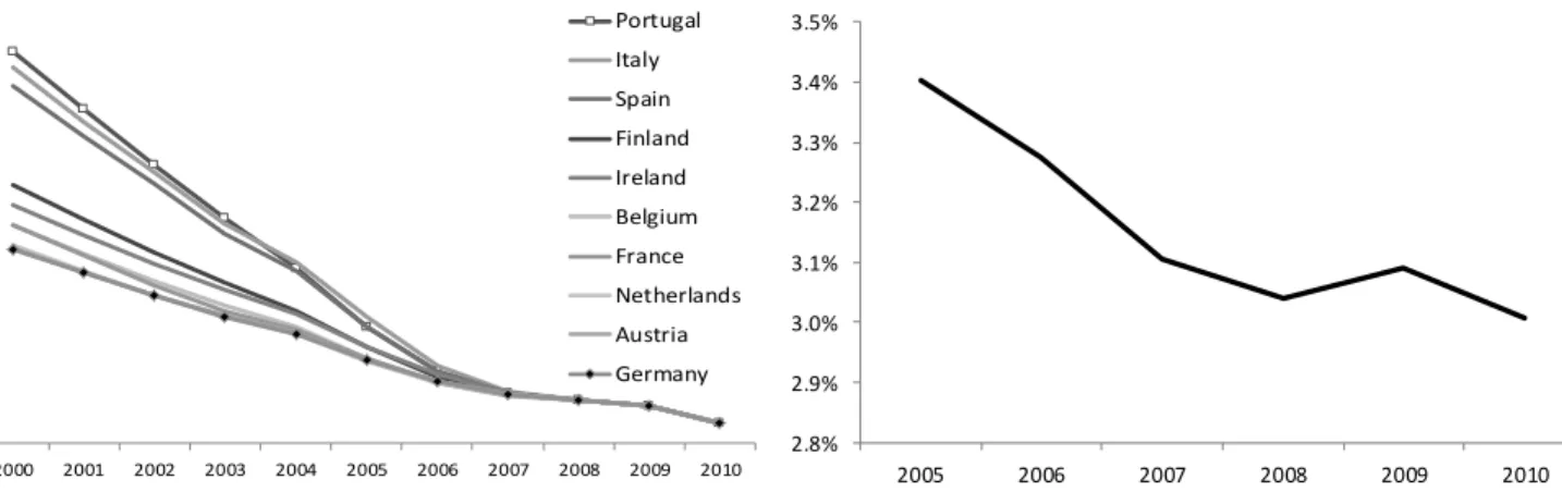
Reverting to the inertia of average rates for portfolios of fixed-rates assets or liabilities, the gradual amortization of old transactions may actually have larger impacts than yearly changes of market rates. This effect shall depend on the roll-over spread between long term rates observed for the preceding years and spot long term rates. We found no analysis of such effect in the existing literature. For each country of the sample, we have created a synthetic variable AMT10 that represents the evolution of the average rate of a portfolio of 10-year (swaps) transactions of which monthly amortizations are rolled-over by new transactions (a portfolio of 120 tranches, and a constant volume). Fig. 4 shows AMT10 since 2000: a very strong downward trend caused by the gradual amortization of higher rates transactions inherited from the previous years can be observed – and this pattern is still at work albeit now at a slower pace. The trend is even further pronounced for example for Portugal of which rates used to be much higher than other countries’ before the inception of the euro. Introducing AMT10 in our models would nevertheless require the history of loan volumes (for individual banks) as from 1996. Hence we did not embed it, we however believed that such a “heritage” effect is present and explains at least part of the erosion of the net interest rate margins of our sample (Fig. 5) and of euro-area banks in general as commented in the introduction (and shown with Fig. 2). We therefore relied on the constants of our models to capture this erosion.

(14)

14 4.2. Bank specific variables

In order to control the changes of profitability ratios for effects specific to individual banks, and therefore increase the accuracy for external variables, we introduced a set of three bank-specific variables: DEPOSITS measures yearly changes of the proportion of deposits vs. customer loans at year end. DEPOSITS is expected to positively influence income components. ASSETS corresponds to yearly changes of the ratio of total assets over customers loans at year-end. It is expected to control for additional income from higher balance sheet leverage. LOAN GROWTH is the % yearly increase of net customer loans. Since only part of income can be assumed to be linked to customer loans (the denominator of our profitability ratios), it is meant to control for potential dilution or concentration effects due to shifts of loans.

4.3. Model

Regressions are performed with our set of selected external and bank-specific variables. A model is dedicated to each sub-component of net earnings before taxes i.e. the influence of variables is distinctly but consistently assessed for the yearly changes of ratios over customer loans for: net interest income, commissions, trading, loan impairments and expenses. We assess the influence of our variables on the full sample of banks and on the three size samples. Further, we investigate potential country divergences with samples for Germany, France and Italy, of which banks are sufficiently represented.

Fig. 4. AMT10: computation of average rates for synthetic portfolios of 10-year interest rate swaps (with constant duration, amortized swaps are rolled-over with spot rates, e.g. 2000 still benefiting from rates observed in 1990). It illustrates a strong margin erosion effect for banks carrying long term fixed-rate assets not matched with contingent liabilities

4% 5% 6% 7% 8% 9% 10% 2000 2001 2002 2003 2004 2005 2006 2007 2008 2009 2010 Portugal Italy Spain Finland Ireland Belgium France Netherlands Austria Germany

Fig. 5. Average net interest income margin over customer loans (full sample) 2.8% 2.9% 3.0% 3.1% 3.2% 3.3% 3.4% 3.5% 2005 2006 2007 2008 2009 2010

(15)

15 We first tested panel-based approaches for regressing changes in earnings. The tests led us to use neither fixed-effects panels nor random-effects panels. Individual banks do not have significantly different means and GLS estimates would not be consistent (Hausman test). Further, White’s tests on an estimation of coefficients through OLS revealed that heteroskedasticity is present. We thus opted for heteroskedasticity-corrected regressions. Despite the exclusion of candidate external variables which were too correlated (cf. section 4.1), we further checked for collinearity issues with variance-inflation-factors for each explanatory variable. VIFs remain below 2 and therefore below critical values10. The generic expression of the equations we estimated is reported with Equation 1.

j k h t i h k t i k h j t j h h t i,

X

Z

,

C

, (Equation 1)

With h: h-th subcomponent of net earnings before taxes (net interest income, commissions, trading, loan impairments or expenses); i: bank i; t: at time t; Xj: j-th external variable expressed in level; Zk: k-th bank-specific (control) variable expressed in level; C: constant shared by banks for the h-th

subcomponent of net earnings.

As mentioned in the section 4.1, our 2005-2010 period includes important shifts for each variable in 2008 and/or 2009. We have taken this fact into consideration by testing the introduction of time dummies in each sub-component model. Their coefficients do not prove significant.

5. Results

5.1. Net interest income

As reported in Table 3, banks of the full sample as well as of the three sub-samples for sizes are negatively exposed to changes of EONIA. Most banks have therefore, actively or passively, opted for a positive interest rate mismatch: interest rate duration is higher for assets than for liabilities. Medium banks exhibit a higher sensitivity to EONIA (-0.081) than large (-0.034) and small banks (-0.046). This observation complies with the comments of the ECB (2007) about lower interest mismatch of larger banks in Europe. The country-wise investigation reveals a markedly stronger negative coefficient for EONIA of German banks (-0.15) and French banks (-0.12). On the contrary, the coefficient for Italian banks turns out to be positive and as high as 0.20. Italian banks therefore reveal an inversed/negative interest rate mismatch. Models on country samples also exhibit much stronger R2.

10_{VIF(j) = 1/(1 - R(j)^2), where R(j) is the multiple correlation coefficient between variable j and the other explanatory} variables. Minimum possible value of VIF is 1; a VIF above 10 indicates a likely collinearity issue.

(16)

16 The constant of the model is significant and negative for all sub-samples excepting Italian banks. We believe it is likely to capture the erosion effect on fixed-rate assets we described in section 4.1. This assumption is also consistent with the observation of highest negative constants for German and French banks which do conduct positive interest mismatch strategies in a greater extent (higher inertia of assets rates).

The coefficient for DEPOSITS is positive and significant for large and medium banks, which indicates than a larger weight of customer deposits increases the net interest income margin. The absence of significance of DEPOSITS for small banks might be explained by the fact that small banks need to offer more attractive conditions to attract deposits. This assumption would not be necessarily contradictory by the earlier finding of a higher net interest margin small banks (section 3.2). This higher margin can be related to heritage effects on long term assets that we commented. ASSETS (the ratio of total assets over customer loans) has a significant and positive influence on the net interest income margin of banks of the full sample as well as of small and medium banks. Balance sheet leverage through securities portfolios, money-markets transactions or trading books is an additional source of interest margin. As EONIA measures the interest rate mismatch, credit spreads on the leverage shall be the main driver of this contribution although transitory mismatch impacts cannot be excluded (deviations vs. the average sensitivity measured by EONIA). The absence of significance for large banks may be due to a higher weight of non-interest bearing assets such as real estate.

Cluster analyses and associated regressions (not reported in the present paper) further evidence the heterogeneity of the sample regarding the influence of EONIA (besides country effects), with strong interest rate mismatch (positive or negative) for a set of banks and rather strict hedging strategies for others

(17)

17 5.2. Net commissions and fees

GDP significantly and positively impacts commissions and fees of banks of all samples, with one exception for French banks11. The coefficient for the large banks is higher than for medium and small banks (0.0079 vs. 0.0032 and 0.0058), which can be explained by potentially broader and more cyclical ranges of banking products of large banks. EQUITIES has also a significant and positive impact either on banks of the full samples or of size sub-samples. The coefficient for EQUITIES is more than twice higher for large banks (0.0013) than for medium and small banks (0.0006 and 0.0005). It suggests more developed financial services (asset-value based) of large banks; this observation complies with the

11

This exception has been investigated in annual financial statements published on web sites of outlying banks. Several French banks report insurance revenues within commissions as from 2009. Commissions and fees have therefore been artificially lifted in 2009 while French GDP growth, as for other countries, was sharply down in 2009.

Table 3

Results for net interest income, estimation of yearly changes of ratio over net customer loans.

(0) constant -0.0009 *** -0.0008 *** -0.0010 *** -0.0007 *** (p-value) 0.0000 0.0002 0.0000 0.0012 (1) GDP 0.0026 0.0052 0.0071 -0.0043 (p-value) 0.4351 0.3887 0.1057 0.4490 (2) EONIA -0.0507 *** -0.0342 ** -0.0811 *** -0.0465 ** (p-value) 0.0000 0.0178 0.0000 0.0149 (3) EQUITIES -0.0006 * -0.0013 ** -0.0001 0.0000 (p-value) 0.0708 0.0443 0.9180 0.9879 (4) DEPOSITS 0.0013 0.0097 *** 0.0064 ** -0.0013 (p-value) 0.3273 0.0063 0.0122 0.4119 (5) ASSETS 0.0028 *** -0.0005 0.0052 *** 0.0034 ** (p-value) 0.0001 0.7666 0.0000 0.0204 (6) LOAN GROWTH -0.0017 * -0.0020 -0.0013 -0.0017 (p-value) 0.0846 0.1985 0.5602 0.2069

P-value (F) 3.84E-13 6.28E-04 1.52E-14 4.44E-03

Adj. R2 (%) 4.78 3.96 15.06 2.95

(0) constant -0.0009 *** -0.0013 *** 0.0000

(p-value) 4.83E-10 8.17E-07 9.42E-01

(1) GDP 0.0184 *** 0.0338 *** -0.0394 ***

(p-value) 1.50E-07 3.70E-06 1.06E-11

(2) EONIA -0.1508 *** -0.1209 *** 0.2012 ***

(p-value) 7.41E-35 4.45E-13 2.22E-27

(3) EQUITIES -0.0004 -0.0021 ** 0.0005 (p-value) 0.4112 0.0172 0.5148 (4) DEPOSITS 0.0041 0.0055 * 0.0024 (p-value) 0.1712 0.0505 0.5567 (5) ASSETS 0.0060 *** -0.0040 ** 0.0006 (p-value) 0.0009 0.0286 0.8379 (6) LOAN GROWTH 0.0006 -0.0021 -0.0111 *** (p-value) 0.5737 0.2353 5.43E-05

P-value (F) 1.94E-36 1.71E-14 1.11E-25

Adj. R2 (%) 26.26 21.01 43.19

Note: Heteroskedasticity-corrected

regressions applying the methodology of White. *, ** and *** indicate significance levels of respectively 10%, 5% and 1%. GDP corresponds to the yearly changes of domestic GDP growth (volume); EONIA to the yearly changes of average interbank overnight rates (euro) and EQUITIES to the year % increase of domestic stock markets (country benchmark indices). DEPOSITS, ASSETS and LOAN GROWTH are bank-specific variables controlling respectively for the ratios of customer deposits, of total assets over customer loans and for the % yearly increase of customer loans. All banks (263)

Large (88) Medium (88) Sub-samples owing to bank size

Small (87)

Sub-samples owing to country

(18)

18 higher level of commissions of large banks commented in section 3.2. EONIA has no significant

influence on the full sample; however large banks appear negatively impacted by increases. One explanation may lie with fiduciary activities related to interest-rate securities, of which fees are negatively influenced by decreasing market value. This complies with the higher sensitivity of commissions to EQUITIES for large banks.

Regarding bank specific (control) variables, coefficients for DEPOSITS are significant and positive for banks of the full sample as well as for large banks. This observation may further highlight the broader range of products offered by large banks and their higher profitability for commissions. No influence of ASSETS is captured by the model for any of the samples, which indicates that commissions primarily depend on loans, deposits and off-balance financial services while non-customer assets barely generate commissions. LOAN GROWTH is significant and negative for all samples. It is likely to account for the sustained rise of loans to customers (yearly compound increase of 7.5% over 2005-2010) and for a dilution effect on non-loan-related commissions.

Table 4

Results for commissions and fees, estimation of yearly changes of ratio over net customer loans.

(0) constant 0.0000 -0.0002 ** 0.0001 0.0002 *** (p-value) 0.3829 0.0234 0.1264 0.0073 (1) GDP 0.0050 *** 0.0079 *** 0.0032 *** 0.0058 *** (p-value) 0.0000 0.0000 0.0010 0.0000 (2) EONIA -0.0022 -0.0224 *** 0.0065 ** 0.0003 (p-value) 0.3621 0.0000 0.0229 0.9288 (3) EQUITIES 0.0009 *** 0.0013 *** 0.0006 *** 0.0005 ** (p-value) 0.0000 0.0000 0.0000 0.0172 (4) DEPOSITS 0.0013 *** 0.0025 ** 0.0005 -0.0008 (p-value) 0.0026 0.0289 0.5153 0.3216 (5) ASSETS -0.0001 0.0005 0.0001 0.0010 (p-value) 0.4606 0.4185 0.7708 0.1356 (6) LOAN GROWTH -0.0047 *** -0.0040 *** -0.0060 *** -0.0060 *** (p-value) 0.0000 0.0000 0.0000 0.0000

P-value (F) 2.62E-81 1.43E-32 1.42E-31 6.22E-32

Adj. R2 (%) 25.46 30.29 29.53 30.09 (0) constant 0.0000 -0.0003 ** -0.0002 (p-value) 0.3882 0.0107 0.2834 (1) GDP 0.0026 *** 0.0030 0.0170 *** (p-value) 0.0001 0.2732 0.0000 (2) EONIA 0.0119 *** -0.0363 *** -0.0629 *** (p-value) 0.0000 0.0000 0.0000 (3) EQUITIES 0.0007 *** 0.0015 *** 0.0000 (p-value) 0.0000 0.0000 0.9913 (4) DEPOSITS 0.0013 ** 0.0032 *** -0.0030 (p-value) 0.0331 0.0029 0.1544 (5) ASSETS 0.0003 -0.0006 0.0019 (p-value) 0.5875 0.4515 0.1342 (6) LOAN GROWTH -0.0021 *** -0.0027 *** -0.0053 *** (p-value) 0.0000 0.0005 0.0017

P-value (F) 1.23E-39 4.05E-16 7.67E-23

Adj. R2 (%) 28.17 23.05 39.59

regressions applying the methodology of White. *, ** and *** indicate significance levels of respectively 10%, 5% and 1%. GDP corresponds to the yearly changes of domestic GDP growth (volume); EONIA to the yearly changes of average interbank overnight rates (euro) and EQUITIES to the year % increase of domestic stock markets (country benchmark indices). DEPOSITS, ASSETS and LOAN GROWTH are bank-specific variables controlling respectively for the ratios of customer deposits, of total assets over customer loans and for the % yearly increase of customer loans.

All banks (263) Sub-samples owing to bank size

Large (88) Medium (88) Small (87)

Germany (116) France (61) Italy (45) Sub-samples owing to country

(19)

19 5.3. Trading

Regarding the full sample of banks, coefficients for EQUITIES and EONIA are both significant for trading activities. The coefficient for EQUITIES is positive while the one for EONIA is negative, banks have therefore long exposures to both stock markets and interest rates instruments.

The coefficients for EQUITIES are highly significant and positive for all sub-samples. Large banks appear to be more sensitive than medium and small banks (0.0051 vs. 0.0019 and 0.0013). Besides potentially higher proprietary trading activities, large banks may benefit from greater customer trading flows since they seemingly diversified in a greater extent into financial services (as reflected by coefficients of EQUITIES for commissions). EQUITIES coefficients are however noticeably higher than for commissions, indicating that trading generates higher income risks than financial / fiduciary activities for all samples. Large banks also appear more sensitive to EONIA than medium banks, also indicating more intense trading on interest rate instruments. As commented earlier, the IRS10 variable (10-year interest swap rate) was not retained in our models given its high correlation EONIA. No conclusion can therefore be made on the dominant influence of yield curve maturity for interest rate trading. Findings related to EONIA for trading shall therefore rather be interpreted as a general sensitivity to interest rates movements.

DEPOSITS positively influences trading income of banks of the full sample. When regarding size sub-samples, the coefficient of DEPOSITS is however only significant for small banks. It suggests that trading of small banks is more influenced by customer transactions.

(20)

20 5.4. Expenses

Only bank specific variables appear to be significant throughout most sub-samples (sizes and countries). Except for small and Italian banks, DEPOSITS has a significant and positive influence on expenses. It may be explained by acquisition costs of new customers as well as by more stringent cost control when deposits and associated income retreat. Except for small and French banks, ASSETS has a significant positive influence and LOAN GROWTH a significant negative one. Higher balance sheet leverage may indeed incur costs. The negative coefficient for LOAN GROWTH is likely to account for the sustained rise of customer loans, and therefore for a dilution of non-loan related expenses (as already commented for commissions).

Table 5

Results for trading, estimation of yearly changes of ratio over net customer loans.

(0) constant -0.0002 * -0.0002 0.0000 -0.0004 *** (p-value) 0.0598 0.3192 0.7983 0.0001 (1) GDP -0.0072 *** -0.0036 -0.0089 *** -0.0020 (p-value) 0.0000 0.4790 0.0000 0.1413 (2) EONIA -0.0156 ** -0.0477 *** -0.0330 *** -0.0087 (p-value) 0.0321 0.0031 0.0000 0.2088 (3) EQUITIES 0.0023 *** 0.0051 *** 0.0019 *** 0.0013 *** (p-value) 0.0000 0.0000 0.0000 0.0002 (4) DEPOSITS 0.0054 *** 0.0031 -0.0011 0.0041 *** (p-value) 0.0000 0.1648 0.3331 0.0000 (5) ASSETS -0.0044 *** -0.0013 -0.0001 0.0004 (p-value) 0.0000 0.4540 0.8640 0.5698 (6) LOAN GROWTH -0.0017 *** -0.0009 -0.0020 * 0.0009 (p-value) 0.0014 0.1976 0.0561 0.1658

P-value (F) 6.25E-40 9.36E-09 7.29E-13 1.69E-34

Adj. R2 (%) 13.61 9.31 13.44 32.03 (0) constant -0.0002 ** -0.0002 -0.0003 (p-value) 0.0264 0.3756 0.3876 (1) GDP -0.0029 *** -0.0018 -0.0202 *** (p-value) 0.0003 0.7882 0.0003 (2) EONIA -0.0011 -0.0308 -0.0761 *** (p-value) 0.7736 0.1033 0.0001 (3) EQUITIES 0.0010 *** 0.0057 *** 0.0055 *** (p-value) 0.0006 0.0000 0.0000 (4) DEPOSITS -0.0002 0.0034 -0.0036 (p-value) 0.7872 0.1485 0.3492 (5) ASSETS 0.0000 0.0012 0.0078 ** (p-value) 0.9467 0.5209 0.0129 (6) LOAN GROWTH 0.0008 ** -0.0008 0.0032 (p-value) 0.0426 0.4423 0.1986

P-value (F) 2.60E-05 1.81E-12 1.68E-11

Adj. R2 (%) 4.25 18.37 22.52

regressions applying the methodology of White. *, ** and *** indicate significance levels of respectively 10%, 5% and 1%. GDP corresponds to the yearly changes of domestic GDP growth (volume); EONIA to the yearly changes of average interbank overnight rates (euro) and EQUITIES to the year % increase of domestic stock markets (country benchmark indices). DEPOSITS, ASSETS and LOAN GROWTH are bank-specific variables controlling respectively for the ratios of customer deposits, of total assets over customer loans and for the % yearly increase of customer loans. All banks (263) Sub-samples owing to bank size

Large (88) Medium (88) Small (87)

(21)

21 5.5. Loan impairments

Models exhibit a marked influence of GDP on loan impairments, for all samples except German banks, not-IFRS and small banks (mostly German banks). Loan impairments retreat when GDP increases. This observation confirms the findings conveyed by the existing literature on the impact of economic cycles. With a coefficient of -0.030, large banks clearly appear more exposed to GDP than medium (-0.017) and small banks (-0.006). DEPOSITS has a taming i.e. negative influence on impairments of the banks of the full sample as well as large and small banks. A greater solvency of customers is consistent with reduced loan impairments. LOAN GROWTH also reduces impairments; this observation is likely to account for a dilution effect since newly granted loans can be expected to be less subject to immediate impairments.

Table 6

Results for expenses, estimation of yearly changes of ratio over net customer loans.

(0) constant -0.0007 *** -0.0009 *** -0.0005 *** -0.0005 *** (p-value) 0.0000 0.0000 0.0023 0.0051 (1) GDP -0.0044 ** 0.0014 -0.0052 * -0.0078 ** (p-value) 0.0496 0.7191 0.0895 0.0319 (2) EONIA -0.0057 -0.0203 ** -0.0041 0.0017 (p-value) 0.3127 0.0207 0.6555 0.8770 (3) EQUITIES 0.0013 *** 0.0002 0.0022 *** 0.0014 ** (p-value) 0.0000 0.6661 0.0001 0.0192 (4) DEPOSITS 0.0054 *** 0.0102 *** 0.0062 ** 0.0007 (p-value) 0.0000 0.0000 0.0184 0.7246 (5) ASSETS 0.0033 *** 0.0038 *** 0.0028 *** 0.0041 ** (p-value) 0.0000 0.0043 0.0081 0.0128 (6) LOAN GROWTH -0.0068 *** -0.0029 ** -0.0107 *** -0.0102 *** (p-value) 0.0000 0.0117 0.0000 0.0000

P-value (F) 1.81E-53 6.38E-16 9.58E-20 3.05E-16

Adj. R2 (%) 17.69 16.35 19.81 16.82 (0) constant -0.0009 *** -0.0008 *** -0.0008 ** (p-value) 0.0000 0.0000 0.0262 (1) GDP -0.0085 *** 0.0015 0.0056 (p-value) 0.0035 0.8585 0.2165 (2) EONIA -0.0086 -0.0163 -0.0261 * (p-value) 0.3933 0.1505 0.0598 (3) EQUITIES 0.0033 *** 0.0002 -0.0005 (p-value) 0.0000 0.7253 0.4873 (4) DEPOSITS 0.0056 * 0.0053 *** 0.0006 (p-value) 0.0617 0.0008 0.8605 (5) ASSETS 0.0080 *** 0.0002 0.0076 *** (p-value) 0.0010 0.8359 0.0038 (6) LOAN GROWTH 0.0005 -0.0072 *** -0.0109 *** (p-value) 0.5100 0.0000 0.0001

P-value (F) 2.71E-18 1.60E-14 1.08E-10

Adj. R2 (%) 14.35 21.04 21.11

All banks (263) Sub-samples owing to bank size Large (88) Medium (88) Small (87)

(22)

22 The absence of significance of GDP for small/German banks was unexpected since, as commented in section 3.2, loan impairments of small banks are actually the most volatile. As shown by Fig. 6, the marked increase of impairments of small banks in 2006 despite a favorable environment, followed by sharp cuts in 2007 and the modest rise in 2008 despite more challenging economic conditions are further striking. This may highlight earnings smoothing strategies by smaller banks. Given our short time series, no variable for smoothing was considered in the models. We also tested our sample by distinguishing IFRS and non IFRS banks. The model for IFRS banks delivers to the highest R2. IFRS indeed provide with a uniform definition of credit default. They also restrain the room for smoothing through impairments, primarily since general provisions (neither specific to loans nor to portfolios of loans) are not allowed. Further, calculation of provisions under IFRS converges with LGD models used by Basle2-IRBA banks for computing risk-weighted assets. IFRS banks exhibit the highest (negative) coefficient for GDP. This higher coefficient for large banks may not necessarily be interpreted as a higher risk but as a better capture of GDP impacts by models. The higher coefficient for large banks may however also indicate more credit risk exposure with loans to corporates and other little collateralized exposures such as consumer lending.

Table 7

Results for loan impairments, estimation of yearly changes of ratio over net customer loans.

(0) constant 0.0004 *** 0.0002 * -0.0001 0.0006 ** (p-value) 0.0066 0.0814 0.7307 0.0314 (1) GDP -0.0173 *** -0.0302 *** -0.0168 ** -0.0056 (p-value) 0.0000 0.0000 0.0255 0.4183 (2) EONIA -0.0018 -0.0118 -0.0070 -0.0148 (p-value) 0.8458 0.3073 0.7200 0.4222 (3) EQUITIES 0.0002 -0.0002 0.0005 0.0005 (p-value) 0.6743 0.7180 0.6007 0.5728 (4) DEPOSITS -0.0054 *** -0.0026 * -0.0041 -0.0081 *** (p-value) 0.0000 0.0854 0.1407 0.0084 (5) ASSETS -0.0001 -0.0003 0.0005 0.0063 ** (p-value) 0.8269 0.8052 0.4828 0.0124 (6) LOAN GROWTH -0.0026 *** -0.0009 * 0.0039 * -0.0063 *** (p-value) 0.0000 0.0893 0.0663 0.0004

P-value (F) 3.60E-14 7.39E-10 3.02E-02 2.85E-03

Adj. R2 (%) 5.14 10.45 1.81 3.19 (0) constant -0.0003 0.0004 * 0.0012 *** (p-value) 0.1909 0.0840 0.0010 (1) GDP -0.0008 -0.0270 *** -0.0333 *** (p-value) 0.8745 0.0057 0.0000 (2) EONIA -0.0031 0.0038 -0.0237 (p-value) 0.8505 0.7912 0.1569 (3) EQUITIES -0.0014 0.0004 0.0000 (p-value) 0.1258 0.6501 0.9907 (4) DEPOSITS 0.0031 0.0034 * -0.0055 (p-value) 0.5263 0.0558 0.2068 (5) ASSETS -0.0015 -0.0015 -0.0006 (p-value) -0.0015 0.2713 0.8134 (6) LOAN GROWTH -0.0034 0.0003 -0.0060 *** (p-value) 0.2162 0.6758 0.0049

P-value (F) 5.98E-01 4.70E-03 8.91E-08

Adj. R2 (%) 0.24 4.15 15.72

All banks (263) Sub-samples owing to bank size Large (88) Medium (88) Small (87)

(23)

23

6. Sensitivity of net earnings to external variables : sub-component regressions vs. direct regressions

As commented in the previous sections, regressions evidence a significant influence of economic and financial variables as well as of control variables. The set of graphs presented in Fig. 6 also reports on the good capture by models of average yearly changes of profitability ratios of individual banks. Although the influence for individual banks may vary around the regression values, our variables seem to address systematic impacts on earnings in a relevant manner - excepting for loan impairments of medium and small banks.

(24)

24 We further assessed the total sensitivity of banks to our economic and financial variables and to our bank-specific variables. For each variable, we report on a total “combined” coefficient i.e. its assumed overall impact on net earnings. In order to assess the robustness of our sub-component models, we compare these combined coefficients with coefficients obtained through direct regressions of net earnings. Results are reported in Table 8.

For the full sample of banks, the combined coefficient for GDP (on net earnings) is positive and stands at 0.0222. The total contribution of gross income (sum of net interest income, commissions and trading) to the coefficient is positive but the main contribution is from loan impairments (0.0173). The coefficient for GDP returned by the “direct” regression of net earnings is very close: 0.0218. The total coefficient for EONIA is negative (-0.061) with contributions of both net interest income (dominating) and trading. The coefficient for EONIA returned by the “direct” regression of net earnings is also close: -0.068. The total coefficient for EQUITIES is positive (0.0010) with contributions of both trading

(dominating) and commissions. The coefficient for EQUITIES returned by the “direct” regression of net earnings is higher (0.0029 vs. 0.0013).

For large of banks, the combined coefficient for GDP stands at 0.0384 and is therefore higher than for the full sample of banks. The difference is primarily due to the higher sensitivity of loan impairments. Consistently, the coefficient for GDP returned by the “direct” regression is higher than for the full sample of banks (0.0523 vs. 0.0218). Both combined and direct coefficients for EONIA are higher than the ones for the full sample of large banks. Whereas EONIA effect on net interest income is somewhat lower (less interest rate mismatch), the sensitivity of trading is clearly higher (-0.0477 vs. -0.0156). The combined coefficient for EQUITIES is as high as 0.0051 and compares very closely with the direct coefficient of 0.0049. Both stand above coefficients for the full sample of banks, the difference is driven by a higher trading exposure.

For medium banks, the combined coefficient for GDP stands at 0.0235, and is therefore lower than for large banks. The lower sensitivity of loan impairments primarily explains the spread. The lower direct coefficient of GDP confirms this direction. The direct coefficient for EQUITIES is not significant. It also supports our combined coefficient of -0.0002 for EQUITIES which appears neglectable when compared to the one for large banks.

(25)

25 For small banks, the direct coefficient for GDP confirms the much lower combined coefficient and, further, is not significant. GDP impacts shall however probably not be neglected as commented in section 5.6, estimates are associated with a modest fit of models for impairments (cf. section 5.5). Our null combined coefficient for EQUITIES complies with by the low and insignificant direct coefficient. The direct model only identifies two significant variables for small banks: EONIA (-0.0474) and LOAN

GROWTH (0.0093). Interestingly, our combined coefficients are very close for these two variables (respectively -0.0418 and -0.0096).

Overall, our models for sub-components seem robust and confirmed by “direct” models on net earnings. Besides, deviations of combined coefficients between the samples are also supported by direct models. Hence we could confirm that GDP positively impacts net earnings primarily through loan impairments and with most noticeable impact for large banks. Excepting for medium and small banks, EQUITIES also supports net earnings primarily through trading activities. EONIA negatively affects net earnings of banks for all samples, essentially as a result of interest rate mismatch but also of trading for large and medium banks.

(26)

26 Table 8.

Summary for sub-component coefficients and combined total (illustrative) coefficients, comparison with direct models for net earnings

A+B+C-D-E (combined coefficient) All banks constant -0.0009 *** 0.0000 -0.0002 * 0.0004 *** -0.0007 *** -0.0007 -0.0006 *** GDP 0.0026 0.0050 *** -0.0072 *** -0.0173 *** -0.0044 ** 0.0222 0.0218 *** EONIA -0.0507 *** -0.0022 -0.0156 ** -0.0018 -0.0057 -0.0609 -0.0680 *** EQUITIES -0.0006 * 0.0009 *** 0.0023 *** 0.0002 0.0013 *** 0.0010 0.0029 *** DEPOSITS 0.0013 0.0013 *** 0.0054 *** -0.0054 *** 0.0054 *** 0.0080 0.0040 * ASSETS 0.0028 *** -0.0001 -0.0044 *** -0.0001 0.0033 *** -0.0049 0.0006 LOAN GROWTH -0.0017 * -0.0047 *** -0.0017 *** -0.0026 *** -0.0068 *** 0.0013 0.0021

P-value (F) 3.84E-13 2.62E-81 6.25E-40 3.60E-14 1.81E-53 1.03E-12

Adj. R2 (%) 4.78 25.46 13.61 5.14 17.69 4.6256 Large banks constant -0.0008 *** -0.0002 ** -0.0002 0.0002 * -0.0009 *** -0.0005 -0.0006 ** GDP 0.0052 0.0079 *** -0.0036 -0.0302 *** 0.0014 0.0384 0.0523 *** EONIA -0.0342 ** -0.0224 *** -0.0477 *** -0.0118 -0.0203 ** -0.0721 -0.0845 *** EQUITIES -0.0013 ** 0.0013 *** 0.0051 *** -0.0002 0.0002 0.0051 0.0049 *** DEPOSITS 0.0097 *** 0.0025 ** 0.0031 -0.0026 * 0.0102 *** 0.0077 0.0111 ** ASSETS -0.0005 0.0005 -0.0013 -0.0003 0.0038 *** -0.0048 -0.0037 LOAN GROWTH -0.0020 -0.0040 *** -0.0009 -0.0009 * -0.0029 ** -0.0031 -0.0023 *

P-value (F) 6.28E-04 1.43E-32 9.36E-09 7.39E-10 6.38E-16 1.67E-12

Adj. R2 (%) 3.96 30.29 9.31 10.45 16.35 13.09 Medium banks constant -0.0010 *** 0.0001 0.0000 -0.0001 -0.0005 *** -0.0003 0.0000 GDP 0.0071 0.0032 *** -0.0089 *** -0.0168 ** -0.0052 * 0.0235 0.0169 ** EONIA -0.0811 *** 0.0065 ** -0.0330 *** -0.0070 -0.0041 -0.0964 -0.0746 *** EQUITIES -0.0001 0.0006 *** 0.0019 *** 0.0005 0.0022 *** -0.0002 0.0008 DEPOSITS 0.0064 ** 0.0005 -0.0011 -0.0041 0.0062 ** 0.0036 -0.0021 ASSETS 0.0052 *** 0.0001 -0.0001 0.0005 0.0028 *** 0.0018 0.0014 ** LOAN GROWTH -0.0013 -0.0060 *** -0.0020 * 0.0039 * -0.0107 *** -0.0026 -0.0058 *

P-value (F) 1.52E-14 1.42E-31 7.29E-13 3.02E-02 9.58E-20 2.49E-04

Adj. R2 (%) 15.06 29.53 13.44 1.81 19.81 4.44 Small banks constant -0.0007 *** 0.0002 *** -0.0004 *** 0.0006 ** -0.0005 *** -0.0009 -0.0002 GDP -0.0043 0.0058 *** -0.0020 -0.0056 -0.0078 ** 0.0130 0.0062 EONIA -0.0465 ** 0.0003 -0.0087 -0.0148 0.0017 -0.0418 -0.0474 * EQUITIES 0.0000 0.0005 ** 0.0013 *** 0.0005 0.0014 ** 0.0000 0.0009 DEPOSITS -0.0013 -0.0008 0.0041 *** -0.0081 *** 0.0007 0.0094 0.0055 ASSETS 0.0034 ** 0.0010 0.0004 0.0063 ** 0.0041 ** -0.0056 0.0000 LOAN GROWTH -0.0017 -0.0060 *** 0.0009 -0.0063 *** -0.0102 *** 0.0096 0.0093 ***

P-value (F) 4.44E-03 6.22E-32 1.69E-34 2.85E-03 3.05E-16 5.80E-07

Adj. R2 (%) 2.95 30.09 32.03 3.19 16.82 7.49

NII (A)

Coefficients of sub-component models

Direct model

(regression) Coefficients for net earnings

LOAN IMPAIR. (D) EXPENSES. (E) TRADING (C)

(27)

27

7. Relative impacts of external variables on net earnings

In this chapter, we analyze the effective impacts of variables between 2005 and 2010. For each variable, we apply our combined coefficients described in chapter 6 i.e. we estimate the total yearly effects of single variables throughout the sub-components of net earnings. For each size sample, the estimated impacts shall therefore be regarded as for an “average” bank.

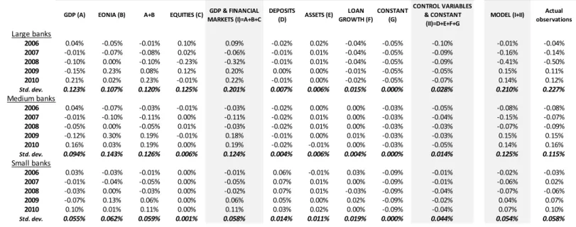
As reported in Table 9, column (I), large banks were the most impacted by economic and financial market factors over 2005-2010. GDP, EONIA and EQUITIES together contributed a standard deviation of 0.201% to net earnings over loans. They induced a much lower volatility for small banks (0.058%), less than half the one for medium banks (0.124%). This observation for small banks, and in a certain extent for medium banks, should however be prudent given the modest fit of the model for their loan impairments commented in section 5.5.

The higher volatility induced for large banks is largely associated with EQUITIES. The sharp correction of stock markets in 2008 (-44%, country-weighted) caused for instance an estimated cut of 0.23% of net earnings over customer loans. The volatility contribution of EQUITIES (0.125%) is only slightly higher than GDP (0.123%) and EONIA (0.107%). When associating GDP with more traditional banking owing to its dominant influence on loan impairments (cf. chapter 6), traditional banking was therefore barely less volatile than equity-related activities. But EQUITIES brought little diversification vs. GDP and EONIA (column A+B).

Still regarding large banks, the volatility induced by GDP is slightly reduced by EONIA through interest rate mismatch and trading. Although they are also sensitive to EONIA, the same mitigation effect is not observed for medium and small banks. But, as earlier mentioned in section 5.5 and visible with Fig. 6, their GDP impacts may be biased by smoothing. It is worth noticing that, despite more challenging economic conditions (GDP cuts) since 2007, the ECB only started to cut its repo rate by the end of 2008 – but then sharply. EONIA therefore provided no relief in 2008 but, in 2009, offset the impacts of GDP for both 2008 and 2009 for all size samples.