Behavioral biases and the representative agent
Elyès Jouini
CEREMADE, Université Paris Dauphine, Place du Maréchal de Lattre de Tassigny,
75 775 Paris cedex 16, jouini@ceremade.dauphine.fr;
phone: + 33 1 44 05 42 26; fax: + 33 1 44 05 48 49. Clotilde Napp
CRNRS-DRM and Université Paris Dauphine, Place du Maréchal de Lattre de Tassigny,
75 775 Paris cedex 16; clotilde.napp@dauphine.fr,
phone: + 33 1 44 05 46 42; fax: + 33 1 44 05 48 49 March 17, 2011
Abstract
In this paper, we show that behavioral features can be obtained at a group level even if they do not appear at the individual level. Starting from a standard model of Pareto optimal allocations, with expected utility maximizers but allowing for heterogeneity among individual beliefs, we show in particular that the representative agent has an inverse S-shaped probability distortion function as in Cumulative Prospect Theory (CPT).
JEL Codes : G11; D81; D84; D87; D03;
Keywords: behavioral biases, probability weighting function, representative agent.
1
Introduction
In this paper, we analyze a model of Pareto optimal allocations with von Neuman Morgenstern utility maximizing agents. Agents are heterogeneous, in the sense that they might di¤er in their beliefs. At the aggregate level, the social welfare function of this economy is characterized by a social/representative belief. We show that we retrieve, at the aggregate level, behavioral properties even though they are not assumed at the individual level. The group acts as a behavioral agent and this behavioral property at the aggregate level is generated by heterogeneity alone.
We start by introducing natural notions of optimism and pessimism and we assume that beliefs are heterogeneous enough in order to allow for optimistic as well as pessimistic agents in the initial set of von Neuman Morgenstern utility maximizing agents. In such a setting, we obtain that the representative agent1 can neither be everywhere optimistic nor everywhere pessimistic; she is optimistic for the good states of the world and pessimistic for the bad states of the world. As in the SP/A Theory of Lopes (1987), the representative agent behaves as if she had fear (need for security) for very bad events and hope (desire for potential) for very good events. The representative agent puts more weight on extreme events. We show that the distribution of outcomes from the representative agent point of view is portfolio dominated by the objective distribution. This means that heterogeneity generates doubt at the aggregate level.
1
See Jouini and Napp (2007) for the existence and the construction of such a representative agent.
This e¤ect is reinforced when agents are more risk tolerant or when there is more heterogeneity among agents.
The representative agent distorts the objective distribution of aggregate endowment. We analyze this distortion and we show that the distortion function (de…ned as the transformation of the objective decumulative distribution function into the decumulative distribution function of the representative agent) is inverse S-shaped as is the probability weighting function in Cumulative Prospect Theory. We show that we are able to …t relatively well standard probability weighting functions of the Cumulative Prospect Theory literature (Tversky and Kahneman, 1992, Tversky and Fox, 1995, Prelec, 1998, among others). According to Gonzalez and Wu (1999) terminology, attractiveness at the aggregate level is directly related to the average level of optimism while discriminability is related to beliefs heterogeneity.
The idea that an inverse S-shaped probability weighting function may be the result of aggre-gation has been put forward by Luce (1996). However, in this last reference, the aggreaggre-gation is of statistical nature (the author considers an average of di¤erent subjects) while our aggregation is in terms of representative agent.
Note that we don’t pretend to retrieve all features of CPT on the aggregate belief. We only retrieve one of the three main features of CPT, namely the inverse S-shaped probability distribution weighting function (the other two being the presence of a reference point and the presence of loss aversion). We have introduced heterogeneity on the beliefs only and it is then natural to retrieve behavioral properties that deal with beliefs only.
The paper is organised as follows. Section 2 presents the model. Section 3 analyses the properties of the belief of the representative agent. Section 4 proposes extensions and remarks. All proofs can be found in the electronic web appendix2.
2
The Setting
We consider an economy with a single consumption good and with agents who have the same utility function but heterogeneous beliefs. Aggregate endowment in the consumption good is described by a random variable e de…ned on a probability space ( ; F; P ) : We let I denote the set of heterogeneous agents3. We assume that the common utility function is CRRA with derivative given by u0(x) = x 1. Each agent has a subjective belief Qi and wants to maximize
her von Neumann Morgenstern utility for consumption of the form Ui(c) = EQi[u (c)] : We
let Mi denote the density of Qi with respect to the probability P , hence agent i’s utility for
consumption can equivalently be written in the form Ui(c) = E Miu (c) :
In such an economy, we consider the aggregate utility function U de…ned as the solution of the following maximization program
U (e ) P max
i2Iyi=e
X
i2I
iE Miu(yi)
where ( i) are given positive weights. The aggregate utility function corresponds to the value
of the social welfare function at the Pareto optimum when agent i is granted a weight i by a
social planner. The index i may also represent a group of agents with common beliefs Mi; yi then represents the total consumption of the group and i the sum of the weights granted by
the social planner to the individuals in the group. When the social planner grants the same weight to all the agents in the economy, the weight i represents the proportion of agents that
have the same belief Mi: From a social planner point of view, the aggregate utility function corresponds to the highest social utility level among all possible endowment distributions across agents.
2http://www.ceremade.dauphine.fr/~jouini/ 3
The number of agents can be …nite or in…nite. In the case of an in…nite number of agents, sums are replaced by integrals.
The function U can represent the utility of a group I of agents (household, village com-munity) assuming that each member of the group has speci…c beliefs Qi and that the group
behavior results from a bargaining process leading to a Pareto e¢ cient allocation of resources (yi). The bargaining process attaches a weight i to each member of the group ; these weights
can then be interpreted as bargaining power. This is for instance the approach adopted in the collective model of the household developed by Chiappori (1988, 1992)4. This approach is to be contrasted with non cooperative or strategic approaches, as in e.g., Ulph (1988), which rely on Cournot-Nash equilibria.
We obtain the following representation result.
Proposition 1 Representative Agent
The aggregate utility for consumption is given by U (e ) = E [M u(e )] with M = X i2I i Mi !1 (1)
for i= i: The representative agent belief is then given by M = Pi2I i Mi 1.
This means that, at the Pareto optimum, the aggregate utility is given by the utility of a representative agent endowed with an average belief (and the same utility function as each of the agents). In particular, if all the agents share the same belief, then the representative agent will share this common belief. If we think of e as a given prospect for the group I of agents, the aggregate utility U (e ) corresponds to the social welfare associated with the optimal allocation of e across the members of the group and is given by the utility of the representative agent.
In the case where the distribution of e for agent i admits a density5 (for all i 2 I) denoted by fiand where the distribution of e under the probability P also admits a density denoted by
f , the following Corollary characterizes the density of e for the representative agent. Since we don’t have E [M ] = 1 (except in the speci…c logarithmic utility setting) we need …rst the follow-ing technical de…nition. We say that the distribution of a random variable X admits a “density fX for the representative agent” if for all function h, we have E [M h (X)] =R h (x) fX(x) dx:
Moreover, in order to analyse the relative weights of the di¤erent states of the world from the representative agent point of view, we introduce the probability measure Q de…ned by
dQ dP
M E[M ].
Corollary 2 The distribution of e admits the following density for the representative agent
fM = X
i2I i fi
!1=
which is a power average of the initial densities. In particular, for = 1; the distribution of e for the representative agent is a mixture of the individual subjective distributions.
As an immediate consequence of Corollary 2, we get that for any measurable real-valued function '; the distribution of ' (e ) admits the density fM;' = Pi2I i fi;' 1= for the representative agent where fi;'denotes the density of the distribution of ' (e ) for agent i: This implies in particular that in the case = 1; if each agent anticipates a normal distribution on log e , then the distribution of log e is a mixture of normal distributions for the representative agent.
4See also Abdellaoui et al. (2010) where the groups under consideration are couples, as well as Mazzocco and
Saini (2011) and Chiappori et al. (2010) where the groups under consideration are village communities.
5In other words, the distribution of e under Q
iis absolutely continuous with respect to the Lebesgue measure.
3
Behavioral properties of the group
In this Section, the aggregate endowment e as well as the individual beliefs Mi are considered
as given and we analyze the distributional properties of e from the group point of view. In particular, we show that this agent distorts the distribution of e as would a CPT agent. At this stage, our representative agent is an expected (subjective) utility maximizer as can be seen through Proposition 1. In Section 4 we will see that more sophisticated constructions lead to agents who distort the distribution of any prospect as would a CPT agent.
3.1 Illustrative examples
The next two simple examples illustrate some qualitative properties of the endowment distribu-tion from the representative agent point of view. The proofs can be found in the web appendix. Example 1. Let us assume that all utility functions are logarithmic ( = 1): We have
EQ[e ] =X
i2I
iEQi[e ] ;
which means that the mean at the aggregate level is given by an arithmetic average of the individual means. The variance is given by
V arQ[e ] =X i2I iV arQi[e ] + V ari E Qi[e ] ; where V ari E Qi[e ] P i2I i EQi[e ] 2 P i2I iEQi[e ] 2
measures beliefs (on the mean) heterogeneity. This means that the variance at the aggregate level is given not only by an arithmetic average of the individual variances, but also by an additional term related to beliefs dispersion. The variance is “increased” at the aggregate level and this increase is proportional to the level of beliefs heterogeneity: beliefs heterogeneity generates “doubt”.
Example 2. Let us assume that the objective distribution of aggregate endowment is lognormal with e P ln N ( ; 2) and that we have two equally weighted groups of agents, both with
lognormal subjective distributions for aggregate endowment, e Qi ln N ( i; 2) for i = 1; 2:
The distribution of log e for the representative agent is not Gaussian and when agents’beliefs are heterogeneous enough (j 1 2j > p2 ), the distribution of log e is bimodal (see Figure 1).
When = 1+ 2
2 ; the distribution of log e for the representative agent is Portfolio Dominated 6
by the objective distribution. Hence, aggregate endowment e is considered as more risky by the representative agent than it actually is. In particular, we have V arQ[log e ] > V arP [log e ]. This last property still holds for general ( i). Figures 1 and 2 illustrate these conclusions in di¤erent settings. Note that Figure 1 is similar to Figure 8.2 in Shefrin (2005). For > 0 and associated representative agent probability measures Q and Q 0; we have dQ
dQ 0 = h ; 0(e ) where
h ; 0 is symmetric with respect to 1+2 2, decreasing before 1+2 2 and increasing after 1+2 2.
A higher level of risk tolerance induces then a portfolio dominated shift in the representative agent’s distribution. In particular, V arQ[log e ] increases with the level or risk tolerance : The interpretation is the following. When there is heterogeneity, each agent consumes a larger proportion of aggregate endowment in states of the world that she considers more likely. This leads to heterogeneous allocations and generates variance at the aggregate level. However, this e¤ect is counterbalanced by risk aversion. Consequently, the higher the level of risk tolerance,
6Let us recall that a distribution f dominates a distribution g in the sense of Portfolio Dominance (f P Dg)
if we haveRu0(x)(x a)f (x)dx = 0 =)Ru0(x)(x a)g(x)dx = 0for any real number a and any non-decreasing concave function u: This concept has been introduced in the context of portfolio problems by Landsberger and Meilijson (1993) and further studied by Gollier (1997). It characterizes the changes in the distribution of the returns of the risky asset that lead to an increase in demand for the risky asset irrespective of the risk-free rate. It is then related to the degree of riskiness. See also Jouini and Napp (2008).
the more heterogeneous the members of the group are in their optimal allocations. Figure 2 illustrates this result.
3.2 Qualitative properties
This section deals with notions of optimism and pessimism at the individual as well as at the representative agent level. For normal distributions N ( i; 2), there is a natural order on
the set of possible densities induced by the natural order on the means ( i). Agents with a larger (resp. smaller) i can be referred to as more optimistic (resp. pessimistic). For general distributions (with densities), we de…ne relative pessimism/optimism in the following way. If we assume that P is the objective probability, then we are also able to introduce absolute notions of pessimism/optimism.
De…nition 1 For i; j 2 I; agent i is said to be more optimistic than agent j and we denote it by fi <opt fj if and only if ffij is nondecreasing. The optimism relation <opt is an order on the set
(fi)i2I: If P is the objective probability, then agent i is said to be optimistic (resp. pessimistic)
if fi
f is nondecreasing (resp. nonincreasing).
De…nition 1 can be rephrased in terms of Monotone Likelihood Ratio Dominance (MLR)7
: agent i is more optimistic than agent j if the distribution of e for agent i (i.e., under Qi)
dominates the distribution of e for agent j (i.e., under Qj) in the sense of the MLR. For a
given agent i; if we let gi denote the transformation of the objective decumulative distribution
function F into the agent’s subjective decumulative distribution function Fi, i.e. such that
Fi= gi F; it is easy to check that ffi is nondecreasing (resp. nonincreasing) if and only if gi is
convex (resp. concave). This means that our concept of optimism/pessimism is the analog, in the expected utility framework, of the concept of optimism/pessimism introduced by Diecidue and Wakker (2001) in a RDEU framework. Other concepts of optimism/pessimism have been proposed in the literature. In particular, Yaari (1987), Chateauneuf and Cohen (1994) and Abel (2002) propose a de…nition based on First Stochastic Dominance8. Note that MLR dominance is stronger than FSD.
A MLR dominated shift for a given distribution reduces the mean and if fi <opt fj then
we have EQi[e ] EQj[e ]. This last condition characterizes the MLR dominance when we
restrict our attention to a family of lognormal distributions with the same variance parameter and we then retrieve that agent i is more optimistic than agent j if and only if i> j: In that case, optimistic (resp. pessimistic) agents are then characterized by i > (resp. i < ) as in Shefrin (2005).
Proposition 3 We suppose that there are at least one optimistic agent denoted by fopt and
one pessimistic agent denoted by fpess in the set I of agents: We also assume that lim+1foptf =
lim0fpessf = +1 and lim0foptf = lim+1fpessf = 0:
1. The representative agent can neither be optimistic, nor pessimistic, i.e. fM
f is non monotone.
2. The representative agent overestimates the weight of the “good states of the world” (high values of e ) as well as the weight of the “bad states of the world” (low values of e ), i.e. fM(x) f (x) for x x and fM(x) f (x) for x x where x and x are given real
numbers.
7
This concept is widely used in the statistical literature and was …rst introduced in the context of portfolio problems by Landsberger and Meilijson (1990). More precisely, Landsberger and Meilijson (1990) showed that in the standard portfolio problem a MLR shift in the distribution of returns of the risky asset leads to an increase in demand for the risky asset for all agents with nondecreasing utilities.
8More precisely, in an expected utility framework Abel (2002) de…nes pessimism by the condition F i F
(First Stochastic Dominance) that corresponds to the condition gi Idintroduced by Chateauneuf and Cohen
(1994) in a RDEU setting.
3. If one of the agents denoted by foptmax is more optimistic than all the other agents and if one of the agents denoted by fpessmax is more pessimistic than all the other agents, then the representative agent behaves like the most pessimistic individual for low values of e and behaves like the most optimistic individual for high values of e ; i.e. fM +1 foptmax and
fM 0 fpessmax:
By de…nition, fopt
f (resp. fpess
f ) is nondecreasing (resp. nonincreasing). In Proposition 3,
we slightly reinforce these conditions by further assuming that the values of fopt
f (resp. fpess
f )
range from zero to in…nity. Notice that these conditions are satis…ed in the case of lognormal distributions.
It appears from this proposition that as long as there are optimistic as well as pessimistic agents in the set I of agents, the representative agent apprehends the aggregate endowment distribution like the individual agents considered in the behavioral economics and/or psychology literature. Indeed, she puts more weight on small probability events with large consequences as in the Cumulative Prospect Theory of Tversky and Kahneman (1992). She has fear (need for security) for very bad events and hope (desire for potential) for very good events as in the SP/A Theory of Lopes (1987). Everything works then as if the representative agent distorted the objective distribution of e . In the next section, we analyze more precisely how this distortion operates.
3.3 The distortion function
With the same notations as in Section 2, we denote by ge the distortion function that
trans-forms the objective decumulative distribution function of e into the aggregate decumulative distribution function of e ; i.e. such that ge (
R1
x f (s)ds) =
R1
x f
M(s)ds: The next proposition
characterizes the shape of ge .
Proposition 4 1. In the lognormal setting with log e Qi N i; 2 for i = 1; :::; N and if
the set I is made of both optimistic and pessimistic agents then the function ge is inverse
S-shaped: concave then convex.
2. In the general setting, if there are at least one optimistic agent fopt and one pessimistic
agent fpess with lim+1foptf = lim 1 fpess f = +1 and lim 1 fopt f = lim+1 fpess f = 0 and if
ge is continuously twice di¤ erentiable on [0; 1], then ge is concave for small probabilities,
and convex for high probabilities.
The function ge then has the same shape as the probability weighting function of the
Cumulative Prospect Theory. This is in particular illustrated in Figure 3. A variety of methods have been used to determine the shape of the probability weighting function. Tversky and Kahneman (1992), Tversky and Fox (1995) and Prelec (1998) among others specify parametric forms (respectively ! (p) = p
[p +(1 p) ]1= , ! (p) =
p
[ p +(1 p) ]1= and ! (p) = exp ( log p ))
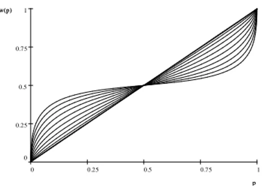
and estimate them through standard techniques. Figure 4 permits to show that, with a well chosen distribution of agents’ characteristics, we obtain a distortion function that perfectly …ts Prelec (1998)’s function. Wu and Gonzalez (1996, 1998) and Abdellaoui (2000) avoid the potential problems of parametric estimation and directly derive from experimental studies the shape of the probability weighting function at the aggregate or individual level. The results of all these studies are (mostly) consistent with an inverse S-shaped weighting function, concave for small probabilities, and convex for moderate and high probabilities.
In the lognormal setting, if we denote by i the quantity i = i ; it is interesting to
remark that the distortion function ge only depends on the is and on the relative proportions is and is independent of and . In other words, the distortion function only depends on how
much the agents deviate from the objective mean in terms of standard deviation. 6
3.4 Discriminability, attractiveness and the shape of the probability weight-ing function
Gonzalez and Wu (1999) exhibit two main features for the shape of the probability weighting function in the context of CPT: discriminability and attractiveness. In this section, we relate these two features of the probability function to the individual beliefs of the agents and to shifts in the distribution of these beliefs9.
Attractiveness characterizes the absolute level of the function. Indeed, an inverse S-shaped function can be completely below the identity line, can cross the identity line at some point or can be completely above the identity line. Betting on the chance domain is more attractive when the graph of the probability weighting function graph is more “elevated”. The de…nition of attractiveness is expressed in terms of First Stochastic Dominance (FSD) of subjective den-sities. In particular, since FSD is weaker than MLR, a more optimistic representative agent is associated with a more attractive distortion function.
When all agents have logarithmic utility functions, attractiveness at the representative agent level increases with FSD shifts in the weights granted to the di¤erent agents, i.e. when the weight granted to the more attractive density functions is increased. Hence, attractiveness at the representative agent level increases with the weight granted to the more optimistic agents. This is illustrated in Figure 5. This property can be extended to power utility functions if we replace FSD shifts in the distribution of agents’density functions by MLR shifts.
Discriminability corresponds to the fact that people become less sensitive to changes in prob-ability as they move away from a reference point. In the probprob-ability domain, the two endpoints 0 (certainly will not happen) and 1 (certainly will happen) serve as reference points and under this principle, increments near the endpoints of probability loom larger than increments near the middle of the scale.
When the level of disagreement among agents increases, then the representative agent focuses more on the endpoints of the probability domain and is less sensitive to probability variations in the middle of the scale. Figure 6 illustrates this result. It shows, in the setting with two agents, that discriminability decreases with the level of disagreement. When both agents agree on the objective distribution, the probability weighting function is linear. When the agents disagree, one of them overestimating the average payo¤ by twice the standard deviation and the other underestimating it by twice the standard deviation, we obtain a function that approaches a step function.
4
Extensions and remarks
We have seen that starting from a standard model with optimistic as well as pessimistic vNM agents and a given aggregate endowment e , we obtain, at the representative agent level, be-havioral properties such as an inverse S-shaped distortion function ge . Furthermore, the
rep-resentative agent behaves like the most optimistic agent for high levels of wealth and like the most pessimistic agent for low levels of wealth. These results are consistent with the …ndings of Abdellaoui et al. (2010) who obtain probability weighting functions for couples that are inverse S-shaped. They also obtain that couple preferences are closer to women’s preferences (the most pessimistic ones) at low probability levels (and low outcomes) and to men’s preferences (the most optimistic ones) at high probability levels (and high outcomes).
Our results can be extended in the following directions (see the web appendix for more detailed explanations).
9
Formal de…nitions and results can be found in the web appendix.
4.1 Hyperbolic discounting
It has been shown in the literature that « hyperbolic discounting » is obtained at the aggregate level when one considers groups with heterogeneous exponential discount rates. This means that in the same way as we have obtained a behavioral bias on the belief of the representative agent if heterogeneity of the beliefs is assumed at the individual level, a behavioral bias is obtained on the time preference rate of the representative agent if heterogeneity of the time preference rates is assumed at the individal level. This result has been obtained in the literature through di¤erent approaches : Reinschmidt (2002), or Weitzman (1998, 2002) have adopted a certainty equivalent approach, Gollier and Zeckhauser (2005) and Nocetti et al. (2008) a Benthamite/Pareto optimal approach, and Lengwiler (2005) an equilibrium approach. All these papers are in a deterministic setting, with no divergence in the beliefs of the agents. In our setting, by assuming heterogeneity on the beliefs (as in Section 3) and on the time preference rates of the agents, we can retrieve the behavioral properties at the aggregate level both on the belief of the representative agent and on her time preference rate.
4.2 Cumulative Prospect Theory
In Section 3, the individual beliefs were given independently of the aggregate endowment e and the distortion function ge was speci…c to e . A dual approach consists in considering speci…c
individual beliefs Qi, in order to obtain a distortion function that is independent of a given
aggregate endowment (or a given prospect) e as in CPT.
Consider …rst the space E of normal distributions, and suppose that for all e in E with e N ( ; 2), the belief Qi;e of agent i is such that e Qi;e N ( i;
2) with
i = + i
for some parameter i. Then we can show that the representative agent is a CPT agent over
the space E of normal distributions, in the sense that there exists a probability weighting function g such that for all e in E with density fe ; we have U (e ) =
R
fe ; (s) u (s) ds where
g Rt1fe (s) ds =
R1
t fe ; (s) ds; moreover, if there exist at least one pessimistic and one
optimistic agent, then the distortion function g is inverse S-shaped.
This result can be easily extended to general distributions to obtain a CPT agent over the space of all random variables, by relying on the fact that any random variable is distributed as a function of a given normally distributed variable.
4.3 Dynamic Issues
Our model might be embedded in a dynamic setting. Consider as in …nancial models a di¤usion setting: We denote by W a Brownian motion and we assume that e follows the stochastic di¤erential equation with constant parameters det = +12 2 etdt+ etdWt. The distribution
of et is then, for all t; lognormal of the form log et N ( t; 2t): Let us assume as in Section 4.2 that agents’deviation from the objective mean is constant in terms of standard deviation, i.e., that the subjective distributions are of the form log N ( it; 2t) with it = t + i pt:
There exists a probability weighting function g that distorts the objective distribution into the distribution of the group. We check that this function is independent of t and the behavior of the group is then consistent across time.
4.4 Experimental issues
Luce (1996) put forward the idea that an inverse S-shaped probability weighting function is not necessarily an individual feature but may be the result of statistical aggregation. Andersen et al. (2010) explores models where the agents are allowed to make errors in their decision process, that is to say models where the probability to choose the lottery with the highest utility level is not 1. They show through an experiment involving 158 subjects and 9311 choices, that there is virtually no evidence of probability weighting. It would be interesting to test in the same
environment if familily of subjects for which there is no evidence of probability weighting at the individual level may exhibit probability weighting when they are grouped into subgroups and asked to take collective decisions within the subgroup.
A way to do that would be to select couples and to present them with the same tasks as in Harrison and Rutström (2008) or Andersen et al. (2010), …rst separately and then jointly following the experimental procedure described by Bateman and Munro (2005). The aim would then be to estimate on these data a model of decision making that allows for a probability weighting function that could be of the form
w(p) = p
(p + (1 p) )1=
as in Andersen et al. (2010). In this last reference and on the basis of individual choices, the estimate of is 0.986 with a 95% con…dence interval between 0.971 and 1.002. The hypothesis that = 1 has a 2 value of 2.77 with 1 degree of freedom, implying a p-value of 0.096. It
would be interesting to estimate on the basis of couples’joint choices and to analyze if it is signi…cantly di¤erent from 1.
4.5 Average rationality and aggregate rationality
We have obtained, at the aggregate level, some anomalies which are absent at the individual level. As in Bateman and Munro (2005) we may wonder if conversely, the group may eliminate some individual anomalies. For instance, group decision making may reduce framing e¤ects. However, as far as probability weighting is concerned, the group has an inverse S-shaped function even when its members are on average rational (see Figure 3). This fact has been explored further in Jouini and Napp (2010). This paper explores a …nancial model with 2 agents that are on average rational. It is shown that the equilibrium prices and allocations are on average equal to those that would be obtained in a rational framework. However, the equilibrium characteristics exhibit systematic deviations from the rational characteristics.
References
Abel, A., 2002. An exploration of the e¤ects of pessimism and doubt on asset returns. Journal of Economic Dynamics and Control, 26, 1075-1092.
Abdellaoui, M., 2000. Parameter-free Elicitation of Utilities and Probability Weighting Functions. Management Science 46, 1497-1512.
Abdellaoui, M., L’Haridon, O. and C. Paraschiv, 2010. Individual vs collective behavior: an experimental investigation of risk and time preferences in couples, Working Paper, HEC, Paris. Andersen, S., Harrison, G., Lau, M. and E. Rutström, 2010. Behavioral econometrics for psychologists, Journal of Economic Psychology, 31, 553-576.
Bateman, I., and A. Munro, 2005. An experiment on risky choice amongst households. Economic Journal, 115, 176-189.
Chateauneuf, A. and M. Cohen, 1994. Risk seeking with diminishing marginal utility in a nonexpected utility model. Journal of Risk and Insurance, 9, 77-91.
Chiappori, P.-A., 1988. Nash-bargained households decisions: a comment. International Economic Review, 29, 791-796.
Chiappori, P.-A., 1992. Collective labor supply and welfare. Journal of Political Economy, 100, 437-467.
Chiappori, P.-A., Samphantharak, K., Schulhofer-Wohl, S. and R. Townsend, 2010. Hetero-geneity and risk sharing in Thai villages, Working Paper.
Diecidue, E. and P. Wakker, 2001. On the Intuition of Rank Dependent Utility. Journal of Risk and Insurance, 281-298.
Gollier, C., 1997. A Note on Portfolio Dominance. Review of Economic Studies, 64, 147-150. Gollier, C. and R. Zeckhauser, 2005. Aggregation of heterogeneous time preferences. Journal of Political Economy, 113, 4, 878-898.
Gonzalez, R., and G. Wu, 1999. On the shape of the probability weighting function. Cog-nitive Psychology, 38, 129-166.
Harrison, G. and E. Rutström, 2008. Expected Utility Theory And Prospect Theory: One Wedding and A Decent Funeral. Experimental Economics, 12, 133-158.
College of Business Administration, University of Central Florida, 2005.
Jouini, E., and C. Napp, 2007. Consensus Consumer and Intertemporal Asset pricing with Heterogeneous Beliefs. Review of Economic Studies, 2007, 74, 1149-1174.
Jouini, E., and C. Napp, 2008. On Abel’s concept of doubt and pessimism. Journal of Economic Dynamics and Control, 32, 3682-3694.
Jouini, E. and C. Napp, 2010. Unbiased Disagreement in Financial Markets, Waves of Pessimism and the Risk-Return Tradeo¤. To appear. Review of Finance.
Landsberger, M., and I. Meilijson, 1990. Demand for risky assets: a portfolio analysis. Journal of Economic Theory, 50, 204-213.
Landsberger, M., and I. Meilijson, 1993. Mean Preserving Portfolio Dominance. The Review of Economic Studies, 60, 475-485.
Lengwiler, Y., 2005. Heterogeneous patience and the term structure of real interest rates. American Economic Review, 95, 890-896.
Lopes, L., 1987. Between hope and fear: the psychology of risk. Advances in Experimental Social Psychology, 20, 255-295.
Luce, R. D., 1996. When Four Distinct Ways to Measure Utility Are the Same. Journal of Mathematical Psychology, 40, 297-317.
Mazzocco, M., and S. Saini, 2011. Testing E¢ cient Risk Sharing with Heterogeneous Risk Preferences. Forthcoming, American Economic Review.
Nocetti, D., Jouini, E., and C. Napp, 2008. Properties of the social discount rate in a Benthamite framework with heterogeneous degrees of impatience. Management Science, 54, 1822-1826.
Prelec, D., 1998. The Probability Weighting Function. Econometrica, 66, 497-527.
Reinschmidt, K.F., 2002. Aggregate Social Discount Rate derived from individual discount rates. Management Science, 48, 307-312.
Shefrin, H., 2005. A Behavioral Approach to Asset Pricing. Elsevier.
Tversky, A., and C.R. Fox, 1995. Ambiguity Aversion and Comparative Ignorance. Quar-terly Journal of Economics, 110, 585-603.
Tversky, A., and D. Kahneman, 1992. Advances in Prospect Theory: Cumulative Repre-sentation of Uncertainty. Journal of Risk and Uncertainty, 5, 297-323.
Ulph, D., 1988. A general non cooperative Nash model of household consumption behavior, Working Paper 88-205, Dept of Economics, University of Bristol.
Weitzman, M., 1998. Why the far distant future should be discounted at its lowest possible rate. Journal of Environmental Economics and Management, 36, 201-208.
Weitzman, M., 2001. Gamma discounting. The American Economic Review, 91, 260-271. Wu, G., and R. Gonzalez, 1996. Curvature of the probability weighting function. Manage-ment Science, 42, 1676-1690.
Wu, G., and R. Gonzalez, 1998. Common consequence conditions in decision making under risk. Journal of Risk and Uncertainty, 16, 115-139.
Yaari, M.E., 1987. The Dual Theory of Choice under Risk. Econometrica, 55, 95-115.
Figure 1: In this …gure, we have represented in black the consensus belief in a log-utility agents setting. A proportion of 47% of the agents believe that log e N (0; 1) and the remaining 53% believe that log e N (2:5; 1): The beliefs of these two categories of agents are represented in grey.
Figure 2: In this …gure we represent the consensus belief for 3 di¤erent levels of risk aversion. We assume that a proportion of 47% of the agents believe that log e N (0; 1) and the remaining 53% believe that log e N (2:5; 1): The upper curve corresponds to = 2; the lower curve to = 0:8 and the middle curve to = 1: An increase of increases the distance between the peaks and their size.
Figure 3: In this …gure we represent in black the representative agent probability weighting function in a model with two logarithmic utility agents. One of them overestimates the ob-jective mean by one standard deviation and the other one underestimates it by one standard deviation. We also represent in grey the individual probability weighting functions (the concave one corresponds to the optimistic agent).
Figure 4: In this …gure we represent Prelec’s function exp( ( ln p) ) with = 0:73 that cor-responds to a standard speci…cation. We also represent the probability weighting function corresponding to a model with two log-utility agents. The …rst one underestimates the ob-jective average by 120% of the standard deviation and has a weight of 30%. The second one overestimates the objective average by 60% of the standard deviation and has a weight of 70%.
1 0.75 0.5 0.25 0 1 0.75 0.5 0.25 0 p w(p) p w(p)
Figure 5: In this …gure we represent the probability weighting function of the representative agent in a model with logarithmic utility agents. In the upper curve, the optimistic and the pessimistic agents are equally weighted. In the lower curve, the pessimistic agents have a 60% weight and the optimistic ones have a 40% weight. Attractiveness decreases with the weight granted to the pessimistic agents.
1 0.75 0.5 0.25 0 1 0.75 0.5 0.25 0 p w(p) p w(p)
Figure 6: The probability weighting function for di¤erent levels of divergence of belief. Both agents agree on a normal distribution but one of them overestimates the objective mean by times the standard deviation while the other one underestimates it by times the standard deviation. The value of ranges from 0 to 2. The discriminability decreases with (in other words the curvature increases with ).
Behavioral biases and the representative agent. Web appendix.
Elyès Jouini
CEREMADE, Université Paris Dauphine, Place du Maréchal de Lattre de Tassigny,
75 775 Paris cedex 16, jouini@ceremade.dauphine.fr;
phone: + 33 1 44 05 42 26; fax: + 33 1 44 05 48 49. Clotilde Napp
CRNRS-DRM and Université Paris Dauphine, Place du Maréchal de Lattre de Tassigny,
75 775 Paris cedex 16; clotilde.napp@dauphine.fr,
phone: + 33 1 44 05 46 42; fax: + 33 1 44 05 48 49 February 11, 2011
1
Proofs of the main paper propositions
Proof of Proposition 1
At the Pareto optimum, we have
iMiu0(yi) = q
for some random variable q: It follows that yi = q iMi hence e =X i2I q iMi = q X i2I 1 iMi and yi = e iM i P i2I[ iMi] : We have then X i2I iE Miu(yi) = X i2I iE 2 4Mi iM i 1 P i2I[ iMi] 1 1u(e ) 3 5 = E 2 4 P i2I iMi P i2I[ iMi] 1 1u(e ) 3 5 = E 2 4 " X i2I iMi #1= u(e ) 3 5
and U (e ) = E [M u(e )] with M = Pi2I i Mi 1= . Proof of Corollary 2
We have E [M h (e )] = E 2 4 X i2I i Mi !1= h (e ) 3 5 = E 2 4 X i2I i fi f (e ) !1= h (e ) 3 5 = E " P i2I i fi(e ) 1= f (e ) h (e ) # = Z P i2I i fi(x) 1= f (x) h (x) f (x) dx = Z X i2I i fi(x) !1= h (x) dx hence fM = Pi2I i(fi) 1= :
Proofs for Example 2
1. Proof that the distribution of log e is bimodal for j 1 2j > 2 =p and
uni-modal for j 1 2j 2 =p : We have
flog = 1 2 f log 1 + 1 2 f log 2 = 1 2p2 exp (x 1)2 2 2 ! + 1 2p2 exp (x 2)2 2 2 ! :
This function has either two maxima that are symmetric with respect to 1+ 2
2 or only
one maximum at 1+ 2
2 : In the …rst case
1+ 2
2 would be a local minimum. It su¢ ces
then to analyse the sign of the second derivative of flog at 1+ 2
2 : We obtain that the
distribution is bimodal for j 1 2j > 2 =p and unimodal for j 1 2j 2 =p :
2. Proof that for = 1+ 2
2 the distribution of log e is portfolio dominated by
the objective distribution. The ratio between the density of log e under Q and the
density of log e under P is given by fM log flog (x) = 1 2exp 2 (x ) ( 1) + 2 2 1 2 2 + 1 2exp 2x( 2) + 2 2 2 2 2 1
which is clearly symmetric with respect to , decreasing before and increasing after :
Moreover, since the distributions of log e under Q and under P are both symmetric with
respect to , we have EQ[log e ] = EP[log e ] = : These properties give V arQ[log e ] >
V arP[log e ] (see Jouini and Napp, 2008).
3. Proof that for general ( i) ; V arQ[log e ] > V arP[log e ] : For general ( i), fM log
is symmetric with respect to 1+ 2
2 which gives EQ[log e ] = 1 + 2
2 : Furthermore, we
may apply the same reasoning as in 2. to compare the distribution of log e under Q
with the distribution whose density is given by p1
2 exp x 1+ 2 2 2 2 2 : We then have V arQ[log e ] > 2 = V arP[log e ] :
4. Proof that a higher level of risk tolerance induces a Portfolio Dominated shift
in the representative agent distribution. For two di¤erent values and 0 of the risk
tolerance parameter; it su¢ ces to consider f
M log 0
fM log and to apply the same reasoning as in 2.
Proof of Proposition 3 1. If lim1fopt f = lim 1 fpess f = 1 and lim 1 fopt f = lim1 fpess
f = 0 then the
representa-tive agent density function is such that lim 1fM
f = lim1 fM f = 1 and fM f can not be monotone.
2. This is immediate according to lim 1fM
f = lim1 fM
f = 1:
3. It su¢ ces to remark that fM = foptmax maxopt +Pi=1;:::;N i6=opt fi fmax opt 1= : If fi fmax opt is
nonin-creasing for all i then maxopt +Pi=1;:::;N i6=opt
fi
fmax opt
1=
is bounded away from 0 and 1 in 4
the neighborhood of 1 and we have fM 1foptmax: The result at the neighborhood of 1 is obtained similarly. Proof of Proposition 4 1. Let g be given byRu1fM(x)dx = g R1 u f (x)dx : We have fM(x) = g0 R1 u f (x)dx f (u) and g0 Ru1f (x)dx = fM
f (u) : We also have f (u)g00
R1 u f (x)dx = fM f 0 (u) which
gives that the concavity of g is governed by the sign of fM
f 0 : Remark that fM f 0 is
negative in a neighborhood of 1 and then that g00 is positive and g is convex in a neighborhood of 1. Similarly, we have that fM
f
0
is positive in a neighborhood of 1 and then that g00 is negative and g is concave in a neighborhood of 1 : Finally, fM
f
0
is a
combination of exponentials where the decreasing exponentials have a negative weight and
the increasing exponentials have a positive weight. The function fM
f
0
is then increasing.
The function g is then inverse S-shaped: concave then convex.
2. Since g0 Ru1f (x)dx = fM
f (u), we have g0(0) = fM
f (1) = 1: If g00(0) is well de…ned, we
have g00(0) < 0 and hence g00(x) < 0 in a neighborhood of 0: The probability weighting
function is then concave for small probabilities. The result in the neighborhood of 1 is
obtained similarly.
2
Formal de…nitions and results for Section 3.4
The de…nition of attractiveness is expressed in terms of First Stochastic Dominance (FSD). The
probability weighting function g1 is more attractive than the probability weighting function g2
when the subjective density f1 dominates the subjective density f2 in the sense of the FSD.
In our setting, we will say that a (representative agent’s) distortion function g1 associated
with a set I1 of agents is more attractive than a (representative agent’s) distortion function g2
associated with a set I2 of agents if fIM1 dominates fIM2 in the sense of the FSD. Attractiveness
of the distortion function is related to the level of optimism of the representative agent. In
particular, since FSD is weaker than MLR, a more optimistic representative agent is associated
with a more attractive distortion function.
Let ( i) and ( 0i) denote two possible distributions of agents’ density functions. If the set
(fi)i2I of agents’ density functions is totally ordered with respect to the FSD order, we will
say that the distribution ( 0
i) dominates the distribution ( i) in the sense of the FSD if for any
increasing family (fi) ; we haveP 0ifi <F SDP ifi: In other words, the distribution ( 0i) puts
more weight on more attractive distributions. If the set (fi)i2I of agents’ density functions is
totally ordered with respect to the optimism order <opt; we will say that the distribution ( 0i)
dominates the distribution ( i) in the sense of the MLR if whenever fi<optfj we have
0 i i 0 j j:
In other words the ratio between the two densities ( 0i) and ( i) increases with agents’optimism
and, in particular, the distribution ( 0
i) puts more weight on more optimistic agents.
In the next proposition we analyze the impact of shifts in the distribution of agents
char-acteristics on the attractiveness of the distortion function and on the level of optimism of the
representative agent.
Proposition 1 1. For log-utility functions and in the case of lognormal distributions log e Qi
N i; 2 for i = 1; :::; N; with the same variance parameter 2, a FSD shift in the
dis-tribution of the means ( i) increases attractiveness of the representative agent’s distortion
function.
2. For log-utility functions and general distributions, if the set (fi)i2I of agents’density
func-tions is totally ordered with respect to the FSD order then a FSD shift in the distribution of
agents’ density functions increases attractiveness of the representative agent’s distortion
function.
3. For general CARA utility functions and general distributions, if the set (fi)i2I of agents’
density functions is totally ordered with respect to the optimism order <opt then a MLR
dominated shift in the distribution of agents’ density functions increases attractiveness of
the representative agent’s distortion function and the level of pessimism of the
represen-tative agent.
Proof 1. Let us consider a distribution of the means that is described by a density
func-tion h . The associated representative agent cumulative distribution function is given by
1 p
2 2
R
dh ( )Rx1exp (s2 2)2ds: Since the function !
Rx
1exp
(s )2
2 2 ds is decreasing a
FSD shift of h decreases the value of Rdh ( )Rx1exp (s2 2)2ds and leads then to a FSD
dominating distribution function for the representative agent.
2. Let us consider a distribution ( 0
i) and a FSD dominated shift ( i). We want to prove
that P 0iFi P iFi: For a given x; letting xi denote the quantity Fi(x), it su¢ ces to prove
thatP 0ixi P ixi for a nondecreasing family (xi)i2I which is true since ( 0i) dominates ( i)
in the sense of the FSD.
3.Let us consider a distribution ( 0i) and a MLR dominated shift ( i). It su¢ ces to prove
that ( P 0 ifi) 1 (P ifi) 1 is increasing or that P 0 iGi P
iGi is increasing with Gi = fi. Without any loss
of generality, we may assume that all the considered functions are di¤erentiable and let us
consider the derivative of
P 0 iGi P iGi P 0 iGi P iGi 0 = ( P 0 iG0i) ( P iGi) (P 0iGi) (P iG0i) (P iGi)2 = P fi fj i j 0 i i 0 j j G 0 iGj GiG0j (P iGi)2 :
Remark that for fi fj we have Gi Gj and then G0iGj GiG0j 0: Furthermore, for fi fj
we also have 0i i
0 j
j 0 which leads to the conclusion.
When all agents have logarithmic utility functions, attractiveness at the representative agent
level increases with the weight granted to the more attractive density functions. Since FSD is 7
weaker than MLR, attractiveness at the representative agent level increases with the weight
granted to the more optimistic agents. This is illustrated by Figure 5. As shown in Proposition
1, this last property can be extended to power utility functions if we replace FSD shifts on the
distribution of agents’density functions by MLR shifts.
Diminishing sensitivity corresponds to the fact that people become less sensitive to changes
in probability as they move away from a reference point. In the probability domain, the two
endpoints 0 (certainly will not happen) and 1 (certainly will happen) serve as reference points
and under this principle, increments near the endpoints of probability loom larger than
incre-ments near the middle of the scale. This concept is related to the concept of discriminability in
psychophysics literature and can be illustrated by two extreme cases: a function that approaches
a step function and a function that is almost linear.
In our setting we say that a representative agent’s distortion function g1 associated with a
set I1 of agents exhibits more discriminability than a representative agent’s distortion function
g2 associated with a set I2 of agents if there exists x 2 [0; 1] such that g1 g2 for x x and
g1 g2 for x x : In the next proposition we show that the level of discriminability of the
representative agent’s distortion function is closely related to the level of disagreement among
agents.
Let us consider as above a family of agents with lognormal distributions ln N ( i; 2). We
denote by ( i) the support of the distribution of the mean parameter and by ( i) the associated
weights. Recall that a mean preserving spread is de…ned as a modi…cation of the distribution
set ( i) on a set of three locations 1 < 2 < 3 with associated increments 1 0; 2 0
and 3 0 such that P3i=1 i = 0 and P3i=1 i i = 0: A mean preserving spread will be said
symmetric if 1= 3:
Proposition 2 For log-utility functions and in the case of lognormal distributions log e Qi
N ( i; 2), a symmetric mean-preserving spread on the distribution of the means ( i) decreases
discriminability of the representative agent’s distortion function. 8
Proof It is immediate that 1; 2; and 3 can be written in the form 2 h; 2; 2 + h for
some h > 0: For the distribution of individual characteristics ( i) ; the representative agent
distribution function is given by p1
2 2 P i i Rx 1exp (s i)2
2 2 ds: The symmetric mean
pre-serving spread induces a modi…cation of this distribution that is positively proportional to
1 p 2 2( Rx 1exp (s 2+h)2 2 2 2 exp (s 2)2 2 2 + exp (s 2 h)2 2 2 )ds: Simple computations
permit to show that this modi…cation is positive for x 2 and negative for x 2: A
sym-metric mean preserving spread leads then to a distribution function that is above (resp. below)
the original distribution function below a given threshold. We have then an increase of the level
of discriminability.
Intuitively, this proposition means that when the level of disagreement among agents
in-creases, then the representative agent focuses more on the endpoints of the probability domain
and is less sensitive to probability variations in the middle of the scale. Figure 6 illustrates this
result. It shows, in the setting with two agents, that discriminability decreases with the level of
disagreement. When both agents agree on the objective distribution, the probability weighting
function is linear. When the agents disagree, one of them overestimating the average payo¤ by
twice the standard deviation and the other underestimating it by twice the standard deviation,
we obtain a function that approaches a step function.
3
Formal de…nitions and results for Section 4.1
In this section, we extend our framework in order to take into account the impact of time and
of heterogeneous time preference rates across the agents. Aggregate endowment at a given date
t is described by a random variable et: Agents have di¤erent time preference rates ( i) and
di¤erent subjective beliefs Qi: We let Mti denote the density at date t of Qi with respect to the
objective probability P and Dti exp ( it) the discount factor of agent i between date 0 and
date t. As previously, we consider the aggregate utility function U de…ned as the solution of
the following maximization program U (et) =Pmax i2Iyti=et X i2I iE MtiDtiu(yit)
where ( i) are given positive weights. Each agent is then characterized by a belief Mti; a discount
factor Dti and a weight i:
We will say that the characteristics Mti; Dit; i i2I are independent if for almost all states of the world !; Mti(!) ; Dit and i are independent1 as random variables on I: This property
will be, in particular, satis…ed when I can be written in the form I = J K L and when
there exist characteristics Mtj
j2J; D
k
t k2K and ` `2L such that for i = (j; k; `) we have
Mti; Dti; i = Mtj; Dtk; ` : Roughly speaking, this property means that there is no speci…c
correlation between beliefs and time preferences and that the weights granted by the social
planner to the individuals in the economy are independent of their time and belief characteristics.
This condition is, in particular, satis…ed when beliefs and time preferences are independent
and when the agents are uniformly weighted in the social welfare function. This is also the case
when the agents’weights are given by their relative wealth and when wealth, beliefs and time
preferences are independent.
Assuming uniform weights is quite reasonable since there is no particular reason for the
social planner to favor one agent with respect to another agent. The independence of beliefs
and time preference rates is more disputable. They may be positively as well as negatively
correlated, the independence condition may then be analyzed as a central scenario.
We easily obtain the following analog of Proposition ?? in the framework with heterogeneous
time preference rates.
Proposition 3 If the characteristics Mti; Dit; i i2I are independent, then the aggregate utility
1
More precisely, for any real valued (measurable) functions f; g; h de…ned on the real line, we have
1 jIj X i2I f Mi t g Dit h ( i) = jIj1 X i2I f Mi t ! 1 jIj X i2I g Di t ! 1 jIj X i2I h ( i) ! a.e. 10
for consumption is given by U (et) = E [MtDtu(et)] with Mt= 1 jIj X i2I Mti !1 and Dt= 1 jIj X i2I Dit !1 :
The representative agent belief is then given by Mt= jIj1 Pi2I Mti
1
and the representative
agent time discount factor is given by Dt= jIj1 Pi2I Dit
1
:
Proof Replacing Mi by MiDi in the proof of Proposition 1, we easily get that
U (et) = " X i2I iMtiDti #1= :
Now, if the characteristics i; Mti; Dit are independent, then
" X i2I iMtiDti #1= = " 1 jIj X i2I Mti !#1= " 1 jIj X i2I Dit !#1= and X i2I iE MtiDitu(yti) = E 2 4 1 jIj X i2I Mti !1= 1 jIj X i2I Dti !1= u(et) 3 5 :
This means that all the properties established in the previous section on the belief of the
representative agent remain valid.
The properties of the representative agent time preference rate are easy to obtain. Note
that the properties of a “consensus” time preference rate when there is heterogeneity on the
individual time preference rates (and not on the beliefs) have already been studied in varying
contexts. Indeed, the problem of the aggregation of the utility discount rates has been studied by
Reinschmidt (2002) through a certainty equivalent approach, by Gollier and Zeckhauser (2005) 11
and Nocetti and al. (2008) through a Benthamite/Pareto optimal approach, and by Lengwiler
(2005) through an equilibrium approach. All these papers adopt a deterministic setting with no
divergence on the beliefs of the agents. On the contrary our aim here is to derive the properties
at the aggregate level simultaneously on the beliefs and on the time preference rate (and in a
quite general stochastic setting).
We know that the representative agent time discount factor is given by Dt= Pi2I jIj1 Dit
1
where Dit exp ( it) : We introduce the representative agent marginal time preference rate
m as well as the representative agent average time preference rate a; respectively de…ned by
D m(t) Dt0 Dt and Da (t) 1 t log Dt:
The average discount rate corresponds to the rate which, if applied constantly for all
in-tervening years, would yield the discount factor Dt; whereas the marginal discount rate is the
rate of change of the discount factor. It is easy to recover the average discount rate from the
marginal discount rate since a(t) = 1tR0t m(s) ds:
Let us state the following properties of the average and marginal time preference rates.
Proposition 4 Properties of the representative agent time preference rate
1. The representative agent average and marginal time preference rates are given by
D a (t) = 1 t log " 1 N N X i=1 exp ( it) #1= ; D m(t) = N X i=1 exp ( it) PN i=1exp ( it) i:
2. The representative agent time preference rates are lower than the average of the time
preference rates, i.e. D m(t) 1 N N X i=1 i = Dm(0) and Da (t) 1 N N X i=1 i= Da (0)
with strict inequalities when i6= j for some (i; j) in I.
3. “Behavioral Properties” : The representative agent time preference rates are decreasing
with time. Moreover, the asymptotic discount rates are given by the lowest time preference
rate, i.e. limt!+1 Da (t) = limt!+1 Dm(t) = infi( i) : The representative agent behaves
for t large enough like the most patient agent.
Proof We prove the proposition for Dm since it is easy to check that all the derived properties
are inherited by Da (t) = 1tR0t Dm(s) ds: 1. Immediate.
2.The representative agent time preference rate Dm(t) =PNi=1 exp( it)
PN
i=1exp( it) i
is an average
of the is with weights that decrease with i: Such an average is smaller than the equally
weighted average.
3. Denote i = exp ( it). We have d D m(t) dt = P i2I i 2i P i2I i P i2I i i P i2I i 2 which is nega-tive. We have D m(t) = inf+ PN
i6=infexp( ( i inf)t) i
1+PNi6=infexp( ( i inf)t)
and exp ( ( i inf)t) i !10 we have then
D
m(t) ! inf:
These formulas permit explicit computations for speci…c distributions of the individual time
preference rates. For instance, if we assume a Gamma 2 distribution ( ; ) for the is we
obtain
D m(t) =
m2 m + v2t
2As mentioned in Section 2, sums should be replaced by integrals when dealing with continuous distributions.
The density function of a gamma distribution ( ; )is given by ( )x 1exp( x):Its mean m and its variance v2 are respectively given by m = and v2=
2:
where m and v2 respectively denote the mean and the variance of the considered distribution.
It is immediate on this simple example that the marginal discount rate decreases with time and
is hyperbolic as in Weitzman (1998, 2001). Furthermore, the speed of the decrease increases
with the level of heterogeneity v2 as well as with the level of risk tolerance.
The next proposition provides comparative statics results for shifts in the distribution f of
the individual time preference rates:
Proposition 5 1. A FSD (resp. SSD) dominated shift in the distribution f of individual
time preference rates decreases the representative agent average time preference rate D a:
2. A MLR (resp. PD) dominated shift in the distribution f of individual time preference
rates decreases the representative agent marginal time preference rate Dm:
Proof The proof of 1. is inspired from Jouini and Napp (2008) and the proof of 2. is inspired
from Nocetti et al. (2008).
1. We have
D a (t)
1
tln E [exp ( t)]
where E is the expectation operator associated with the distribution of ( i). For a given t; the
function ! exp ( t) is decreasing (and convex) and, by de…nition, a FSD (resp. SSD) shift in the distribution of ( i) decreases the value of E [exp ( t)] and increases Da (t) :
2. We have then
D m(t) =
E [ exp ( t)] E [exp ( t)] :
where E is the expectation operator associated with the distribution of ( i) :
1. Let us now consider P1 and P2; two distributions such that P2 M LR P1: By de…nition,
the density = dPdP21 is nondecreasing in (in other words i ! i and i ! i are
comonotonic). We have then, EP 2[ exp( t)]
EP 2[exp( t)] = EP 1[ exp( t)] EP 1[ exp( t)] = EQ[ ] EQ[ ] where Q is 14
de…ned by a density with respect to P1 equal (up to a constant) to exp ( t) : Since is nondecreasing in , we have EQ[ ] EQ[ ] EQ[ ] ; hence EP2[ exp ( t)] EP2 [exp ( t)] E Q[ ] ; EP1[ exp ( t)] EP1 [exp ( t)] :
Let us assume now that P2 P D P1 and let us consider D;P
2
m (t) and D;P
1
m (t) the
associated representative agent time preference rates: We have D;Pm 2(t) = E
P 2[ exp( t)]
EP 2[exp( t)]
and then EP2hu0( )( D;Pm 2)
i
= 0 with u( ) = exp( t): By de…nition, this implies
EP1hu0( )( D;Pm 2)
i
0 hence D;Pm 2 D;P
1
m :
Second Stochastic Dominance as well as Portfolio Dominance are related to a notion of risk
or of dispersion while First Stochastic Dominance and Monotone Likelihood Ratio Dominance
are related to notions of shifts from low values to high values. Roughly speaking, Proposition 5
introduces the right concepts of dispersion and shifts and shows that more dispersion in agents’
time preference rates as well as shifts to lower values of individual time preference rates decrease
the representative agent’s time preference rate.
4
Formal de…nitions and results for Section 4.2
In this section we show that an individual who evaluates lotteries through the social welfare
function associated with a collection of agents, each of them with speci…c noisy beliefs, distorts
the distribution of the lotteries through an inverse S-shaped weighting function (common to all
lotteries) as in CPT.
We start by considering normal distributions. Let us consider an individual who when facing
a lottery whose payo¤ x is described by a normal distribution N ( ; 2) passes this information for evaluation to separate systems. Each system i has a subjective belief Qi under which x
has a normal distribution N + i ; 2 : The parameter i is …xed independently of x and
characterizes the system i. It might result from noise in the information transmission. In that
case there is no speci…c reason for the average perceived signal to be biased and we should
have P i = 0. We assume that the individual acts like a central planner looking for a Pareto
optimal decomposition of the payo¤s from the lottery among the systems and evaluates the
lottery through the social welfare function, i.e.,
U (x) = maxP
xi=x
X
i
iEQi u(xi) (1)
where the parameters i are the weights granted to the systems by the central planner or the
distribution of the is.
Proposition 6 Consider an individual who evaluates any lottery x in the space X of lotteries
with normal payo¤ s through U (x):
1. The individual is a CPT agent over the space X in the sense that there exists a probability
weighting function g such that, for all lotteries x in X with density fx we have U (x) =
R fx; (s)u (s) ds where g ( R1 t fx(s)ds) = R1 t fx; (s)ds:
2. If there exist at least one optimistic and one pessimistic system, then g is inverse
S-shaped.
3. A MLR shift on the distribution of the is increases attractiveness of the probability
weight-ing function g .
Proof 1. Let x 2 X with x N ; 2 : We have x Qi N + i ;
2 : From
Propo-sition ??, there exists Q such that U (x) = EQ[x] and the density of x under Q is given 16
by fx; (s) = h 1 n PN i=1(fx; i) i1=
where fx; i is the density of x under Qi: We then have
U (x) = Rfx; (s)u (s) ds: It su¢ ces to prove that
R1
t fx; (s)ds is a function of
R1
t fx(s)ds
that does not depend on x; i.e. that does not depend upon and : Let g be the function
de…ned by g p1 2 R1 t exp x2 2 ds = R1 t h 1 n PN i=1 p12 exp (x i)2 2 i1= ds for all t:
The function g is completely de…ned on [0; 1] and by a simple change of variables, we have
g p1 2 R1 t exp (x )2 2 2 ds = R1 t h 1 n PN i=1 1 p 2 exp (x i )2 2 2 i1=
ds for all t and
we then haveRt1fx; (s)ds = g
R1
t fx(s)ds :
2. The function g is the same as in Proposition ??.
3. Direct application of Proposition 1.
This means that a Pareto optimal decomposition leads to an overall (representative agent)
evaluation that corresponds to the valuation that would be provided by a behavioral agent.
The level of discriminability would then be directly related to the level of noise as illustrated in
Proposition 2 in the case of log utility functions. The level of attractiveness would be associated
to the level of systematic bias (if any) as a direct corollary of Proposition 1.
The behavior of the individual and the de…nition of the social welfare function U can be
naturally generalized to any lottery whose payo¤ is a function of a normal distribution. Indeed,
consider a lottery whose payo¤ is of the form v = '(x) where x is normally distributed as above
and where ' is a Borelian function. We may de…ne U (v) by
U (v) = maxP
vi=v
X
i
iEQi u(vi)
where the Qis and the is are the same as for x.
The following result extends the result of Proposition 6 to general lotteries. It relies on
the fact that any random variable is distributed as a function of a given normally distributed
variable.
Proposition 7 Consider an individual who evaluates through U any lottery v = '(x) where x 17
is normally distributed and whose preferences over the set of all possible lotteries only depend
on the distribution of the lottery under consideration. The individual is a CPT agent over the
space of all possible lotteries in the sense that her preferences can be represented by the utility
function U extended to the space of all possible lotteries and there exists a probability weighting
function g such that, for all lottery v with density fv we have U (v) =
R
fv; (s)u (s) ds where
g (Rt1fv(s)ds) =
R1
t fv; (s)ds:
Proof Let v such that v = '(x) where x is normally distributed. By de…nition, we have U (v) =
supPviEQi[u(v
i)]. We denote by fvi the density of v with respect to Qi: By Proposition 1 and
Corollary 2, we have U (v) =R fv; (s)u (s) ds with fv; = P fvi
1
: We clearly have fv; =
'0fx; ' and fvi = '0fxi ' and since
R1 t fx; (s)ds = R1 t P fxi 1 (s)ds = g Rt1fx(s)ds ;
a simple change of variable leads to Rt1fv; (s)ds = g
R1
t fv(s)ds : We have then the result
over the set of transformations of normal distributions.
Let us consider now a random variable v and a normally distributed random variable x: We
know that v has the same distribution as Fv 1[Fx(x)] where Fv 1(p) is de…ned by Fv 1(p) =
inf ft : Fv(t) pg : If the individual has preferences that only depend on the distribution, it
su¢ ces to set U (v) = U ('(x)) with ' = Fv 1 Fx which is perfectly de…ned. We then have
U (x) =Rt1f'(x); (s)u(s)ds withRt1f'(x); (s)ds = g Rt1f'(x)(s)ds and since v is distributed like '(x); we have Rt1f'(x); (s)ds = g Rt1fv(s)ds ; and the result follows.
This corollary provides then the following possible interpretation of CPT: the result of
a possibly noisy transmission of the objective distribution to separate (specialized) systems,
the overall evaluation resulting from a social welfare function applied to these systems. The
construction of the Qis in the general case is very similar to their construction in the normal case.
The resulting global behavior might then be associated intuitively with a possible behavior of
the systems that consists in describing any random variable in terms of Gaussian distributions.
For instance, a random variable that takes values 0 and 1 with probability 1/2 may be described
that takes value 0 when the Gaussian variable is negative. The process i will then transform this
binomial distribution into a binomial distribution that is equal to 1 when a Gaussian variable
N ( i; 1) is positive -or equivalently when a Gaussian variable N (0; 1) is smaller than i- and
is equal to 0 when the Gaussian variable N ( i; 1) is negative.