Dynamic slope stability and geomorphological site effects : Numerical simulations and back analysis

(1)

HAL Id: tel-02196802

https://pastel.archives-ouvertes.fr/tel-02196802

Submitted on 29 Jul 2019

HAL is a multi-disciplinary open access archive for the deposit and dissemination of sci-entific research documents, whether they are pub-lished or not. The documents may come from teaching and research institutions in France or abroad, or from public or private research centers.

L’archive ouverte pluridisciplinaire HAL, est destinée au dépôt et à la diffusion de documents scientifiques de niveau recherche, publiés ou non, émanant des établissements d’enseignement et de recherche français ou étrangers, des laboratoires publics ou privés.

effects : Numerical simulations and back analysis

Zezhong Zhang

To cite this version:

Zezhong Zhang. Dynamic slope stability and geomorphological site effects : Numerical simulations and back analysis. Earth Sciences. Université Paris sciences et lettres, 2018. English. �NNT : 2018PSLEM074�. �tel-02196802�

(2)

Préparée à MINES ParisTech

DYNAMIC SLOPE STABILITY AND

GEOMORPHOLOGICAL SITE EFFECTS:

NUMERICAL SIMULATIONS AND BACK ANALYSIS

Soutenue par

Zezhong ZHANG

Le 19 Décembre 2018 Ecole doctorale n° 398

Géosciences, Ressources

Naturelles et Environnement

(GRNE)

Spécialité

Géosciences et géo-ingénierie

Composition du jury : Jean-François SEMBLAT ENSTA Président Véronique MERRIEN

Conservatoire National des Arts et Métiers Rapporteur

Luca LE NTI

IFSTTAR Rapporteur

Fréderic L. PELLE T

MINES ParisTech Examinateur

Jean-Alain FLE URISSON

(3)

Résumé

Stabilité dynamique des versants et effets de site d’origine géomorphologique : simulations numériques et rétro-analyses

Lors de séismes, les effets de site peuvent augmenter ou parfois diminuer l'intensité du mouvement du sol car la présence d’un relief ou de dépôts superficiels peut modifier localement le champ d’ondes. Il a également été montré que la réponse du mouvement du sol en un site spécifique affecte fortement la fréquence et la durée du mouvement sismique. De nombreuses études ont montré l'influence de la topographie sur l'amplification de l'accélération en utilisant des méthodes numériques incorporant un modèle de pente, mais la plupart des recherches ne se sont concentrées que sur un ou plusieurs facteurs indépendants qui affectent le mo uvement du sol. Bien que des études sur l'interaction entre la fréquence des ondes sismiques et les caractéristiques topographiques (ou géologique de subsurface) aient été récemment menées, la connaissance de cet effet de couplage lié à la topographie de la pente fait encore défaut. Par conséquent, une investigation plus approfondie de l'amplification due à la topographie des pentes est toujours nécessaire.

Dans cette thèse, des simulations numériques ont d'abord été effectuées avec le logiciel en différences finies FLAC (Itasca) sur un modèle de pente élastique linéaire homogène pour caractériser l'amplification de l'accélération le long de la surface située le long et à l’arrière de la crête d'une pente, et évaluer ainsi l'effet de la topographie sur l'amplification de l'accélération. L'interaction entre la fréquence du signal sismique appliqué à la base du modèle et l'angle et la hauteur de la pente a été particulièrement étudiée. Il a été constaté que le facteur d’amplification de l’accélération varie de manière significative avec l’angle de et la hauteur de la pente, la fréquence et la durée (nombre de cycle) du signal. De plus, l'amplification du mouvement du sol due à la topographie de la pente est influencée de manière significative par l'effet de couplage complexe entre les ondes incidentes et les ondes réfléchies sur la topographie, et qu’elle est fortement contrôlée par le rapport entre la longueur d'onde du signal incident et la hauteur de la pente.

Les simulations numériques sont basées sur une étude géotechnique et une modélisation géomécanique nécessitant de valider les résultats par des comparaisons entre les résultats de modélisations et les données provenant des observations sur le terrain. L’analyse des domaines de fréquence, telle que la densité spectrale et la réponse en fréquence, est un moyen performant pour comprendre les caractéristiques des processus et les divers phénomènes qui ne peuvent pas être expliqués dans le domaine temporel. À cette fin, une étude de la crête du parc Xishan à Zigong au Sichuan en Chine a été réalisée. Les amplifications du site associées au mouvement du sol produit par le séisme de Wenchuan en 2008 ont été évaluées à l'aide de la technique du rapport spectral standard (SSR) et de la méthode d'accélération quadra tique moyenne (arms) dans le domaine temporel. Une analyse numérique à 2D au moyen du logiciel FLAC (Itasca) a été ensuite mise en œuvre et les résultats ont été comparés aux mesures de terrain. Les pics “simulés” des amplifications spectrales sont toujours inférieurs à ceux dérivés des enregistrements de terrain. L'effet d'atténuation important

(4)

sur le mouvement d'entrée pour les hautes fréquences met en évidence le fait qu'un rapport d'amortissement du signal ne représente pas correctement la dissipation d'énergie dans les simulations numériques. Des amplifications significatives se sont produites à des fréquences élevées (> 10 Hz) et sont considérées comme résultant de conditions locales spécifiques telles que la fracturation des roches et les irrégularités géométriques locales. Ces amplifications ne sont pas nécessairement localisées au sommet de la colline.

Enfin, des études paramétriques ont été réalisées avec des modèles élastiques en termes de diverses géométries de pente 2D et de couches géologiques de subsurface pour caractériser les amplifications du mouvement du sol. L’analyse paramétrique a pour but de comprendre le rôle joué par ces couches de surface, l’angle de la pente et la hauteur de la pente sur l’amplification du mouvement du sol, et donc d’évaluer si l’amplification du site peut être responsable du déclenchement du glissement de terrain. Ensuite, l'analyse dynamique sur des modèles de pente pour différentes magnitudes a été effectuée et la stabilité de la pente du site de Las Colinas au Salvador a été évaluée sur la base du déplacement induit. Les résultats numériques ont clairement montré que les effets de site peuvent avoir induit d'importantes amplifications du mouvement du sol qui ont contribué à déclencher des glissements de terra in.

Mots clés : Effets de site topographiques, Simulations numériques, Stabilité des pentes,

(5)

Abstract

Site effects may increase or sometimes decrease ground motion intensity as the local wave field can be modified due to the presence of topographic features or superficial weak materials. Ground motion records at the specific site also showed that the frequency and duration of seismic motion could also be strongly affected. Numerous studies investigated the influence of topography on acceleration amplification using numerical methods incorporating a slope model, but most researches only focused on one or several independent factors that may affect ground motion. Although studies on the interaction between seismic wave frequency and topographic feature (or surface geology) have been recently reported, knowledge of such coupling effects related to slope topography is still lacking. Therefore, a more thorough investigation of amplifications due to slope topography is still needed.

In this research work, numerical simulations using the FLAC software (Itasca)were first conducted with a homogeneous linear elastic slope model in order to characterize the acceleration amplification along the slope surface and behind the slope crest, and then to evaluate the topographic effect on the acceleration amplification. The interaction between the frequency of the seismic input motion applied at the base of the model with the slope angle and height has been deeply investigated. It was found that significant changes in the acceleration amplification factor result from variations in the slope angle and height as well as the signa l frequency and duration. In addition, it has been shown that the ground motion amplification due to slope topography result from complex coupling effects between the input waves and the reflected waves on the topographic features and is highly controlled by the ratio between the wavelength of the input signal and the slope height.

Numerical simulations are based on geotechnical investigations and geotechnical modeling, and it is necessary to validate the results through comparisons between modeling results and field observations. Frequency domain analysis such as spectral density and frequency response are an effective way to understand process characteristics and the various phenomena that cannot be explained in the time domain. For this purpose, a case st udy at Xishan Park ridge in Zigong in China has been studied. Site amplifications associated with the ground motion produced by the 2008 Wenchuan earthquake have been evaluated using the Standard Spectral Ratio (SSR) technique and root- mean-square acceleration (arms) method in time domain. 2D numerical analysis using the finite difference method using the FLAC software (Itasca) has been then performed and results have been compared with monitoring data. The “simulated” peaks of the spectral amplifications are always lower than those derived from the field records. The strong attenuation of input motion at high frequencies highlights the shortcoming that a signal damping ratio does not adequately represent the energy dissipation in numerical simulations. Significant amplifications occurred at high frequencies (>10 Hz) are considered to result from local specific conditions such as rock fracturing and ridge steps; thus they do not necessarily occur at the top of the hill.

(6)

Finally, parametric studies were performed with elastic models in terms of various 2D slope geometries and geological layers to characterize the ground motion amplifications. The purpose of the parametric analysis is to understand the role of the geological layer, slope angle and slope height on the ground motion amplification, and thus to estimate if site amplifications could be responsible for the triggering of the landslide. Then, the dynamic analysis on the slope model for different seismic magnitudes was performed and the evaluation of the Las Colinas slope stability in Salvador was evaluated through the analysis of the induced displacement. The numerical results clearly showed that site effects can have induced significant ground motion amplifications that contributed to triggering landslides.

(7)

Acknowledgements

First of all, I would like to express sincere gratitude to my supervisor, Professor Jean-Alain Fleurisson for providing the opportunity to work with him in MINES ParisTech. I am really grateful to him for his guidance and patient support during the completion of the research works. Without his kind help, I would never be able to complete this study. I also want to thank Professor Frédéric Pellet for his great support in the paper publishing and kind encouragements all these years. My experience working with them was incredibly rewarding and full of a lot of fun.

I gratefully acknowledge the China Scholar Council which provided a Ph.D. scholarship and gave me therefore the chance to study abroad in the Geosciences and Geoengineering Research Department of MINES ParisTech.

I would like to extend my thanks to Dominique Vassiliadis and Véronique Lachasse for their kind assistance and help provided throughout my stay at Fontainebleau. They really helped me a lot in facilitating the administrative procedures of registration and application to the resident card.

My sincere thanks for many reasons also go to my friends and colleagues (Mohamed, Xiangdong, Paule, Thuong, Sara, Hafsa, Aurelien, Hao, Shuaitao and Yubing). We ever did studying, meeting, eating together with a lot of fun. I will surely remember the very nice time spent together with them.

Last, I would like to express my appreciation to my family and Haijing for their unconditional love and continuous support.

(8)

(9)

List of Figures

Figure 1.1: Collapsed buildings during the 2008 Wenchuan earthquake

(http://agnesngoy.blogspot.fr) ... 1

Figure 1.2: Fatality causes for all deadly earthquakes between September 1968 and June 2008.

(a) With deaths from the 2004 Sumatra event; (b) without deaths from the 2004 Sumatra event. (Marano et al., 2010) ... 2

Figure 1.3: Non-shaking fatalities for all deadly earthquakes between September 1968 and

June 2008. (a) With dead people from the 2004 Sumatra event; (b) without dead people from the 2004 Sumatra event. (Marano et al., 2010) ... 3

Figure 1.4: The location of seismological stations near Sourpi and example of observed

ground motions. (a) Section of the ridge, showing the distribution of seismological stations; (b) recorded ground motions (scale of signal amplitude is the same for all the recording) (Pedersen et al., 1994). ... 6

Figure 1.5: The location of seismological stations near Mt. St. Eynard and recorded ground

motions. (a) Section of the ridge, showing the distribution of seismological stations; (b) observed ground motions (Pedersen et al., 1994). ... 7

Figure 1.6: Local topographic map near the Robinwood ridge and example of spectral ratio

analysis. (a) Local topographic map and the distribution of seismological stations on the ridge; (b) spectral ratios derived from an earthquake event A ( M 2.3) at a distance of 14.1 km (Hartzell et al., 1994). ... 8

Figure 1.7: Geophones installed on at the Cedar Hill Nursery and raw recorded accelerations.

(a) Local topographic map, showing the location of the Geophones installed across the ridge; (b) observed accelerations (Spudich et al., 1996). ... 9

Figure 1.8: Topographic map of the study area (a) and observed ground motions for three

components (b). The interval between neighboring curves is 100 m and the maximum altitude is 1300 m (LeBrun et al., 1999). ... 10

Figure 1.9: The portable stations installed along the ridge and the spectral ratios derived for

several sites. The results show that high ground motion amplification is likely to be attributed to the near-surface geology. Legend defines: a) Recent alluvium; b)‘Marnoso-Arenacea’ formation; c) ‘Scaglia’ formation; d) faults; e) seismic stations. (Caserta et al., 2000). ... 11

Figure 1.10: Arrangement of the array in the study area. (a) Location of the epicenter; (b)

topographic map; (c) the profile showing the distribution of the seismometers (Buech et al., 2010). ... 12

(12)

Figure 1.11: The spectral amplitude of the observed ground motions for two horizontal

components. The results identify the high topographic amplification, which is obtained at a frequency of 5 Hz (Buech et al., 2010). ... 12

Figure 1.12: The location of seismic stations used during Phase I of recording (N-S and E-W

cross-sectional profiles of the feature shown for profiles A-A’ and B-B’ , respectively) (Wood, 2013). ... 13

Figure 1.13: Examples of results from Event 17801 Phase I, Stations 1–10, E-W component:

(a) E-W topographic cross section, (b) time records, (c) Fourier amplitude spectra, and (d) standard spectral ratio (Station 1 used as the reference station). Expected topographic frequencies based on simple analytical formulas range from 0.79–2.39 Hz, as indicated by the inset box in (d) (Wood, 2013). ... 14

Figure 1.14: Topographic map of the instrumented ridge, showing the location of seismic

stations 1–10. Cross section A–A′ showing the location of seismic stations placed along a line parallel to the direction of elongation of the ridge. Cross section B–B′ showing the location of seismic stations placed along a line perpendicular to the direction of elongation of the ridge (Stolte et al., 2017). ... 15

Figure 1.15: A comparison of the spectral ratio in the horizontal direction perpendicular to the

axis of elongation of the ridge (Stolte et al., 2017)... 15

Figure 1.16: Seismic response of the hill model subjected SV waves at different frequencies

range. The topographic contour of 5- foot intervals lines are labeled in white (Bouchon and Barker, 1996)... 19

Figure 2.1: Geometry of the numerical model for L1=200 m and L2=500 m, D-H=150m. ... 29

Figure 2.2: Acceleration time history for the Gabor wavelet for the central frequency f=6 Hz.

... 30

Figure 2.3: Acceleration amplification factor along the surface, for slope angle α=20° and

slope height h=50 m subjected to a seismic wave with central frequency f=6 Hz. Three lines with different color represent amplification factors of slopes with sharp corners and round corners... 31

Figure 2.4: Acceleration amplification factor along the surface, for slope angle α=45° and

slope height h=50 m subjected to a seismic wave with central frequency f=6 Hz. Three lines with different color represent amplification factors of slopes with sharp corners and round corners. The green frame encloses the secondary peak. ... 32

Figure 2.5: Propagation of incident SV waves, reflected SV waves and P waves and diffracted

(13)

Figure 2.6: Amplitude ratio of a reflected P wave as a function of the incident angle. The red

arrow points to the critical angle 32.3°. ... 34

Figure 2.7: The maximum amplification factor as a function of distance from the crest. (a)-(h)

Results from numerical analyses of the slope model with varying slope angles ranging from 10° to 45° in case of slope height h=50 m. The blue arrows point to the maximum acceleration amplification and the red frame encloses the secondary peak. ... 36

Figure 2.8: Location of the maximum amplification as a functio n of the slope angle. For slope

angle α>22.2°, the maximum amplification is observed at a short distance behind the crest. ... 37

Figure 2.9: Acceleration amplification factor as a function of distance from the crest in case of

slope angle α=45°. (a)-(h) Results from numerical analyses of the slope model with varying slope height ranging from 20 to 90 m. The blue arrows point to the maximum acceleration amplification. ... 38

Figure 2.10: Acceleration amplification factor as a function of distance from the crest in case

of slope angle α=25°. (a)-(h) Results from numerical analyses of the slope model with varying slope height ranging from 20 to 90 m. The blue arrows point to the maximum acceleration amplification. ... 39

Figure 2.11: Amplification factor as a function of slope angle. Squares represent results of a

slope with the sharp corner; cycles represent results of a slope with corners of small curvature; triangles represent results of slopes with corners of large curvature. ... 40

Figure 2.12: Amplification factor on the ground surface for slope with sharper corners and

slope with round corners (a), the upper round corner and the lower sharp corner (b) and the upper shape corner and the lower round corner (c), for slope angle α=20° and slope height h=50 m, subjected to a seismic wave with central frequency f=6 Hz. ... 41

Figure 2.13: Acceleration amplification factor as a function of slope angle of configurations

subjected to a Gabor wavelet with different frequencies for slope height h=50 m. ... 43

Figure 2.14: Acceleration amplification factor as a function of slope height of configurations

subjected to a Gabor wavelet with different frequencies for slope angle α=45°. ... 44

Figure 2.15: Acceleration amplification factor as a function of distance from the crest of a

slope subjected to a Gabor wavelet with different significant cycles and a Ricker wavelet for a slope angle α=45° and slope height h=50 m... 45

Figure 3.1: Schematic map showing the location of the monitoring stations and local

topography. (a) Bird’s eye view map, indicating the location of the Zigong study area, which is about 246 km away from the epicenter of the 2008, Mw 7.9 earthquake. Several

other active faults that frequently trigger seismic activity are also indicated on the map (Xu et al., 2005; Yang, 2008). (b) Local topographic map, showing the location of the

(14)

accelerographs installed along a profile across the ridge. (c) Section of the ridge, showing the distribution of the accelerographs along the ridge slope. ... 50

Figure 3.2: Acceleration histories recorded by the accelerograph array on the Xishan Park

ridge during the Wenchuan earthquake. The time history recorded at the #2 station is shorter, but this does not affect the results as time histories windowed from 40 s to 80 s were chosen for analysis. ... 52

Figure 3.3: Stages of data processing at the #2 (reference) and #7 stations. (a) Windowed

accelerations, including the maximum peaks of the SV waves; (b) FFT amplitudes of the windowed accelerations; (c) FFT amplitudes smoothed using a digital FFT filter; (d) spectral amplification ratios at #7 in three directions, respectively. ... 53

Figure 3.4: FFT amplitude spectra observed at sites #2-8 and spectral ratios relative to station

#2 for components East (a, d), North (b, e) and vertical (c, f). ... 54

Figure 3.5: FFT amplitude spectra (a, b, c) for sites #1 and #2 in three directions and spectral

ratios between them (d). The results show that there is significant amplification between 7 and 8 Hz, which is correlated to the soil layer resonance frequency. ... 56

Figure 3.6: Propagation of incident SV waves, reflected P waves and SV waves and diffracted

Rayleigh waves near the slope. ... 57

Figure 3.7: Statistical shear wave velocity of the bedrock in the study region. ... 58 Figure 3.8: The FFT amplitude spectra of ground motion obtained from 1D numerical

simulations. ... 58

Figure 3.9: FFT amplitudes of recorded and computed ground motion for each observation

station. Similar trends are observed between the field observations and the numerical results. ... 60

Figure 3.10: Spectral ratios of observed and computed ground motions for each observation

station. ... 61

Figure 3.11: Comparison of spectral amplification ratios for the ridge model subjected to

different input motions... 63

Figure 3.12: Amplification of ground motion in terms of arms ratios at the 8 observation

stations with respect to the reference station (#2) for the NS and EW components of the recorded ground motion and the horizontal ones predicted by the ridge model. ... 65

Figure 4.1: (a) Map showing the location of the Las Colinas landslide and epicentre of the

2001 earthquakes on January 13 and February 13 in El Salvador; (b) a photograph by the United States Geological Survey (USGS) showing the Las Colinas landslide (triggered by the January 13, 2001, Mw=7.7 El Salvador earthquake) that induced long-range movement.

(15)

Figure 4.2: Observed accelerations (a) at Santa Tecla Station, and the corresponding FFT

spectra (b)... 69

Figure 4.3: The 3 groups of slope models that were numerically simulated. (a) Actual slope

model; (b) model with varying slope angle; and (c) model with varying slope height. .... 72

Figure 4.4: The spectra of the horizontal accelerations obtained from the numerical analyses of

the homogenous and layered models subjected to windowed seismic waves. ... 73

Figure 4.5: Horizontal peak ground motion maximum amplification as a function of distance

from the crest (x=0 corresponds the crest). (a)-(h) Results from numerical analyses for the slope model with varying slope angles from 25° to 60°. ... 75

Figure 4.6: Illustration of wave propagation, reflection, diffraction and superposition. ... 76 Figure 4.7: Peak ground motion amplification as a function of the distance from the crest.

(a)-(f) Results from numerical analyses of the slope model with varying s lope heights ranging from 40 m to 150 m. The red frame encloses the secondary peak. ... 77

Figure 4.8: Amplification factor as a function of the distance from the crest of four slope

models with different geological compositions. (a) Homogenous model; (b) the model in Figure 4.3(a) with brown cinders in place of palaeosol and pyroclastic fall deposits; (c) the model in Figure 4.3(a) with brown cinders in place of palaeosol; and (d) the model in Figure 4.3(a)... 78

Figure 4.9: Distribution of peak ground motion amplification along the ground surface behind

the crest of the model in Figure 4.3(a), subjected to a Gabor wavelet with a varying central frequency from 1 Hz to 10 Hz. ... 79

Figure 4.10: Distribution of peak ground motion amplification along the ground surface

behind the crest in the model of Figure 4.3(a), subjected to a Gabor wavelet with varying cycles of 1, 2, 4, 6 and 12... 80

Figure 4.11: Horizontal displacement distribution in the real slope model subjected input

motion with different peak ground accelerations. (a) PGA=0.1 g; (b) PGA=0.2 g; (c) PGA=0.3 g; (d) PGA equals to the original amplitude. ... 81

(16)

List of Tables

Table 2.1: Parameters controlling the shape of acceleration history ... 29

Table 2.2: Curvature radii for the models ... 32

Table 3.1: Material parameters used in the numerical simulations. ... 59

Table 3.2: Seismic recordings used in the numerical simulation... 62

Table 4.1: Material properties used in the numerical simulations (Bourdeau, 2005) ... 71

Table 4.2: Parameters for controlling the number of cycles ... 73

(17)

Chapter 1 Introduction

1.1 Motivation

Each year in the world, natural disasters such as earthquakes, landslides, debris flow, tsunamis, and hurricanes cause severe losses of life and property damages, as well as consequential losses from disruption of commerce and destruction of infrastructure s slowing the aid to the affected population. According to the statistical investigations on disasters between 1947 to 1980 (Abbott, 2008), 450,048 people lost their lives from earthquakes, 4,519 from the tsunami, and 10,841 from landslides: an average of 14,103 fatalities per year from those events.

Earthquake is one of the most destructive natural events that cause huge losses in a short period of time (Figure 1.1). It is estimated that a minimum of 11 million fatalities were due to earthquakes in the past 4000 years (Korup and Clague, 2009). In the past decades, several catastrophic earthquakes around the world, including the 2006 Mw=6.3 Java (Indonesia) earthquake (Matsuoka and Yamazaki,

2006), the 2007 Mw=8 Peru earthquake (Hébert et al., 2009), the 2008 Mw=7.9 Wenchuan (China)

earthquake (Yin et al., 2009), the 2010 Mw=7.0 Haiti earthquake (Hough et al., 2010a), the 2011

Mw=9.0 Tohoku earthquake (Hayes, 2011) and the 2011 Mw=6.3 Christchurch earthquake (Reyners,

2011), have been reported to have induced massive destructions.

Figure 1.1: Collapsed buildings during the 2008 Wenchuan earthquake (http://agnesngoy.blogspot.fr)

Marano et al. (2010) carried out a quantitative analysis of global earthquake casualties using the primary source of detailed fatality information from US Geological Survey’s (USGS) Preliminary Determination of Epicenters (PDE). 1,442,342 documented fata lities for all deadly events including shakings, landslides, tsunamis, missing and other reasons between September 1968 and June 2008, were compiled (Marano et al., 2010). As can be seen from Figure 1.2, 1,133,878 (77.66%) were due to shaking-related causes, 70,525 (4.83%) were due to landslides, 238,385 (16.33%) were due to tsunami,

(18)

430 (0.03%) were due to other causes, 16,423 (1.12%) were listed missing and assumed dead, and 365 (0.02%) were due to undifferentiated causes. However, the 2004 Great Sumatra–Andaman Islands earthquake and tsunami contributed to the majority of tsunami fatalities with more than 227,000 dead people (Telford and Cosgrave, 2006). In order to eliminate the effect of this single event, the statistical analysis without the Sumatra–Andaman Islands event is presented in Figure 1.2b. This allows a better description of the non-shaking fatal injuries distribution for the covered period of time.

Figure 1.2: Fatality causes for all deadly earthquakes between September 1968 and June 2008. (a) With deaths from

the 2004 Sumatra event; (b) without deaths from the 2004 Sumatra event. (Marano et al., 2010)

Figure 1.3 illustrates the part of the fatalities for all deadly earthquakes between September 1968 and June 2008 who are not directly resulting from earthquake shaking. Landslides, which are responsible for 71.1% of the non-shaking deaths, are observed to be the main cause of non-shaking dead people in earthquakes with a removal of the 2004 Sumatra event. In addition, for many specific earthquake events, it is reported that landslides often contribute to more devastation and fatal injuries than direct earthquake effects. For instance, in the 1964 Alaska earthquake, more than 50% of the total cost of damage was caused due to landslides (Wilson and Keefer, 1985). Kobayashi (1981) pointed out that more than half of the fatalities due to earthquakes in Japan between 1964 and 1980 were caused by landslides.

As another example, over 69,000 people lost their lives in the 2008 Mw=7.9 Wenchuan

earthquake and more than 370,000 were reported injured, with over 18,000 listed as missing as of July 2008 (Dai et al., 2011). Hundreds of thousands of landslides were triggered over a broad area during this earthquake. Some of them buried villages or even cities, blocked the roads and dammed the rivers. It was estimated that about 20,000 amongst the 69,000 fatalities are caused due to landslides during the Wenchuan earthquake (Yin, 2008).

(19)

Figure 1.3: Non-shaking fatalities for all deadly earthquakes between September 1968 and June 2008. (a) With dead

people from the 2004 Sumatra event; (b) without dead people from the 2004 Sumatra event. (Marano et al., 2010)

Topographic effects, e.g. the amplification, de-amplification, or frequency modification of ground motion in the vicinity of topographic features, have drawn widespread attention in the scientific community. Certain topographic irregularities scatter, diffract or focus incident seismic waves, resulting in large amplifications or reductions of ground motions. In particular, severe damages at the top of hills or slopes during earthquakes have been noticed to be induced by site effects. Extremely high movement intensities are often observed near topographic irregularities and may be responsible for landslides triggering. A typical example of the observed “topographic effects” is the extraordinary damage patterns on topographic ridges during the 2010 Mw 7.0 Haiti earthquake, where destructions

were concentrated on ridges or other topographic features (Hough et al., 2010a).

Historically, site effects have been observed in a lot of earthquake events, such as the 1989 Loma Prieta earthquake (Wald et al., 1991), and the 2010 Haiti earthquake (Assimaki and Jeong, 2013;

Hough et al., 2010a). In these events, typical ground motion modifications (most of them are amplifications) are observed near topographic irregularities. This suggests that relief morphology, such as hills, slope and ridges, plays a significant role in modifying seismic waves field near the topographic features. The amplification of ground motion due to topography may be also increased by the resonance of seismic wave-field inside the layer depending on soil layer thickness (comparable with the seismic wavelength). Sometimes, the instructive interference occurs due to resonance when seismic waves propagate into the soil layer at a specific frequency (resonance frequency). Furthermore, ground motion amplification may happen related to special reliefs, where different physical phenomena such as wave reflection, infraction or diffraction can occur and could aggravate destruction. It has been reported for a long time by researchers (Bonamassa and Vidale, 1991; Caserta et al., 2000;

Çelebi, 1987; Donati et al., 2001; Griffiths and Bollinger, 1979; Hartzell et al., 1994; Pedersen et al., 1994), that widespread localized damage often occurs at special sites where always consists of topographic irregularities. Both field observations (Caserta et al., 2000; Spudich et al., 1996; Stolte et al., 2017; Tsai and Huang, 2000; Wood, 2013) and numerical studies (Assimaki et al., 2005; Bouchon, 1973; Lenti and Martino, 2012; Sánchez-Sesma et al., 1982; Wong and Jennings, 1975; Zahradník and Urban, 1984) suggest that topographic effects are very important for the seismic hazard evaluation at the top of ridge or very steep hillsides. Earthquake ground shaking, involving effects of local site conditions, could cause huge destructions. Such local conditions must be taken into account when engineers design criteria of any infrastructure project in seismic areas. Especially at special sites such

(20)

as mountainous areas, topographic effects often interact with soil amplification and thus may aggravate the earthquake- induced disaster.

In order to evaluate ground motion amplifications, ground motion amplification factors or spectral amplification factors derived from surface acceleration-time series, are often provided based on the dynamic response of the local site conditions. Researchers have focused on studying the effects of topography on ground shakings by using numerical and analytical methods. These research results give very valuable insights into the understanding of ground motion amplification. It was also shown that many factors, such as topographic geometry, the presence of the soil layer at the slope surface, three-dimensional (3D) topography geometry, wave- field incident angle and orientation, influence the magnitude of ground motion amplifications and even the frequencies at which these effects are observed. These effects are usually evaluated by site response analysis, which refers to the seismic wave propagation from the bedrock to the ground surface. In most cases, one-dimensional (1D) site response analysis is widely used to evaluate the effect of soil conditions on ground motion. It is of practical interest because vertically propagating shear waves (SV) dominate the seismic wave- field. However, in order to assess the topographic effect, two-dimensional (2D) and even 3D numerical analysis must be conducted based on model profile subjected to seismic signal input motion.

Most of the numerical studies are performed using simplified models such as a homogeneous model with idealized 2D geometry or simple 2D model with soil layering. As a consequence, numerical modeling usually gives lower amplifications than those observed in instrumented field studies. There are many reasons, such as the presence of a loose soil layer at the surface, wave- field incident angle and orientation, wave type, and three-dimensional (3D) topography geometry (Geli et al., 1988; Paolucci, 2002; Semblat et al., 2002), for the discrepancies between observed results and numerical results, but the most important of them are uncertainties in the subsurface properties used in numerical simulations and the lack of adequate knowledge of topographic features. In this respect, a few studies have used 3D models with more realistic geological and geomorphological site conditions to compute ground motion amplifications due to surface topography (Chaljub et al., 2010; Lee et al., 2009; Maufroy et al., 2012). Such 3D numerical modeling is supposed to predict ground motion amplifications in a more accurate and realistic way and get results closer to what could be observed in the field, but they are more complex and more time and money consuming than the 2D studies.

Although research works have been done on topographic irregularity, a study on the phenomenon related to small- scale factors, 3D effects, and high- frequency seismic waves, is still needed. In this document, we address the issue of ground motion amplifications due to site effect using numerical models in terms of variation of the geometry and subsurface geology. The effects of topography, geology and input motions are assessed by quantifying ground motion amplification along slope ground surface, and interactions between topographic amplification and surficial soil amplification are also discussed. Numerical simulations have also been performed on two case studies where field measurements were available in order to compare the results of numerical modeling with field data and to study the reason why differences may occur.

1.2 Literature review

Seismic waves have been observed being modified by local geological and topographic conditions for a long time. The phenomena of ground motion modifications are widely known due to site effects and they can result in significant differences in the characteristics of shaking at a given site.

(21)

Site effects mainly include four factors. (1) The stiffness of the soil or rock at the local site (Atkinson and Cassidy, 2000; Bouckovalas and Kouretzis, 2001): Seismic waves travel faster through stiff sediments than through softer ones; when waves spread from deep (often harder) to shallow (softer) rocks, the seismic waves slow down and the amplitude of seismic waves increases as the energy is accumulated. The higher the contrast on stiffness, the larger the seismic amplifications. (2) The presence of a weak soil layer (Assimaki et al., 2005; Bauer et al., 2001): as a consequence of the contrast in the impedance, seismic waves are trapped in soil layers so that it produces higher amplitudes and longer durations. The effect is strongly dependent on the relationship between the wave frequency (wavelength) and the thickness of the soil layer. (3) Topographic conditions (Fukushima et al., 2000; Geli et al., 1988; Meunier et al., 2008; Paolucci, 2002; Spudich et al., 1996): topographic geometries including slopes, ridges, and canyons have a significant influence on the ground motion characteristics and seismic intensity; a higher peak horizontal acceleration is often recorded by accelerometer installed at the top of a ridge or hill than those recorded by nearby accelerographs at surrounding areas. (4) Geologica l structures (Bertrand et al., 2011; Cormier and Spudich, 1984): sedimentary basins and dipping layers are expected to focus or defocus seismic waves and therefore to have a significant effect on ground motion modifications. Seismic waves travelling through faults or sedimentary basins from bedrock with high shear velocity will slow down and get larger amplitude of the earthquake waves. The high density contrast between the sedimentary material in the basin and the surrounding materials induces wave trapping into the basin which will combine and result in stronger and longer ground motion.

1.2.1 Topographic amplification

1.2.1.1 Instrumental observations

Charles Darwin was one of the first to explain the phenomena of fractured and displaced soil on narrow ridges using topographic effects (Barlow, 1933), during the 1835, February 20, Chilean earthquake. Afterward, the observation of churned ground, ground fissures, and overturned boulders near the topographic features subjected to strong ground shaking were attributed to topographic effects (Boore, 1972; Plafker et al., 1971; Ponti and Wells, 1991). Field observations on topographic amplifications have been improved for fundamental data acquisition and have been carried out in many case studies (Hartzell et al., 1994; Pedersen et al., 1994; Spudich et al., 1996). Nowadays the array of velocimeter or strong motion networks can be used to record a given seismic event at different sites and allow to easily compare the ground motion from the same seismic event and thus to evaluate topographic effects.

Topographic amplification can be computed in the time domain based on ratio between the peak ground motion recorded at a given site and those recorded at a reference site, or in the frequency domain by comparing the frequency spectra. However, sometimes physical phenomena related to seismic wave propagation are hard to be explained in the time domain since they are strongly frequency-dependent. Frequency domain analysis such as spectral density and frequency response is an effective way to understand process characteristics and the various phenomena that cannot be explained in the time domain. The Standard Spectral Ratio (SSR) (Borcherdt, 1970) applied on earthquake data are the most frequently used spectral analysis methods. SSR is defined as the spectral ratio of the specific site with respect to a reference site on bedrock. The key step is to choose the available reference site, which cannot be affected by any topographic effects. Based on this idea, topographical

(22)

and geological amplifications that occurred during past earthquakes are investigated by instrumental studies and several cases are presented hereafter.

Pedersen et al. (1994) carried out two field experiments to evaluate local amplification and wave diffraction on a ridge (Figure 1.4). They obtained seismic records of local and regional earthquakes. The recorded ground motions were processed both in the frequency domain and in the time domain. Numerical analyses were also performed with two-dimensional models by the indirect boundary element method for comparison. In the first experiment, amplification ratios of 1.5 to 3 at the ridge top with respect to the base of the ridge were observed by Fast Fourier Transform analysis. It was also observed that amplifications of horizontal components are slightly higher than amplifications in the vertical direction. For different earthquakes, the spectral ratios seem stable. The theoretical spectral ratios from numerical analyses were found in good agreement with observed spectral amplifications.

Figure 1.4: The location of seismological stations near Sourpi and example of observed ground motions. (a) Section

of the ridge, showing the distribution of seismological stations; (b) recorded ground motions (scale of signal amplitude is the same for all the recording) (Pedersen et al., 1994).

In the second experiment, Pedersen et al. (1994) arranged 5 seismological stations along a ridge, which presents a very steep cliff at its top and is filled with soft deposit at the ridge bottom. Recording stations were installed along the slope and numbered 1 to 7 from the top to the bottom. Strong soil amplifications were observed at stations 1, 4, and 5 (Figure 1.5), as the amplitudes of ground motio n recorded at stations 1, 4, and 5 were much larger than those recorded on rock sites (stations 2 and 3). To study the pure topography- induced effects, stations 2 and 3 were selected for spectral ratio analysis. The spectral amplitude ratio at station 3 with respect to station 2 was calculated with a widowed

(23)

ground motion of frequency range larger than 2 Hz. A broadband relative amplification between 2 and 4 Hz was observed for the vertical component.

Figure 1.5: The location of seismological stations near Mt. St. Eynard and recorded ground motions. (a) Section of

the ridge, showing the distribution of seismological stations; (b) observed ground motions (Pedersen et al., 1994).

Severe structural damage and ground cracking on a ridge during the 1989 Loma Prieta earthquake lead to carry out research works focused on site effect evaluation in this region. Hartzell et al. (1994) deployed a dense array of three-component accelerographs on Robinwood ridge 7.3 km northwest of the epicenter for investigating the cause of severe earthquake damage observed on the ridge crest. Ground motions recorded by the array allowed spectral analyses considering the base as a reference site (Figure1.6). Amplification with spectral ratios from 1.5 to 4.5 was observed in frequencies ranging from 1.0 to 3.0 Hz. The reason can be attributed to a combination of local geological effects and topographic amplification. In the higher frequency range, high amplification can be detected up to 5.

(24)

Figure 1.6: Local topographic map near the Robinwood ridge and example of spectral ratio analysis. (a) Local

topographic map and the distribution of seismological stations on the ridge; (b) spectral ratios derived from an earthquake event A (M 2.3) at a distance of 14.1 km (Hartzell et al., 1994).

In order to investigate the cause of a high observed acceleration of 1.78 g at the Cedar Hill Nursery (Figure 1.7), Spudich et al. (1996) installed 21 three-component geophones in six radial lines with an average distance between the sensors of 35 m on the hill. The radial lines are oriented in six directions, which are the north (N), south (S), east (E), west (W), northeast (NE), and southeast (SE). The raw recorded ground motion can also be seen in Figure 1.7. The results identify the directional topographic effect and the resonance frequency at a transverse direction is 4.5 Hz. The amplification ratio of 4.5 at the hilltop is obtained in the horizontal direction. Comparisons of field observations with theoretical results indicate that the 3D shape of the hill and its internal structure are important factors affecting its response.

( b) (

(25)

Figure 1.7: Geophones installed on at the Cedar Hill Nursery and raw recorded accelerations. (a) Local topographic

map, showing the location of the Geophones installed across the ridge; (b) observed accelerations (Spudich et al., 1996).

An experiment for investigating the effects on the seismic ground motion on a hill near Corinth (Greece), with large dimensions of 6 km long, 3 km wide and 700 m high, was performed by LeBrun et al. (1999). In this experiment, 7 accelerometers were installed along the hill, and the recorded ground motions were analyzed with different methods: the standard spectral ratios (SSR) and the horizontal to vertical spectral ratios both calculated on ambient noise (HVNR) and earthquake data (RF). HVNR is based on the spectral ratio between the horizontal and vertical components of a ground motion recorded at the same station. This method is mainly applied to microtremors or, sometimes, to strong motions (Wen et al., 2014) and allows the estimation of the predominant resonance frequency at the local site under consideration. Two assumptions are established for using the HVNR method. The first one is that the vertical component of the tremor is mostly composed of Rayleigh waves. The second one is that the ratio between horizontal and vertical spectra of surface tremor is supposed to be as an approximate transfer function. The experiment results show that the amplification at the resonant frequency (around 0.7 Hz, which is given by f = 0.4∗β/l, with β being the S wave velocity and l being the half- width of the topography (Geli et al., 1988)) is relatively low; however, it is found that a large amplification (up to a factor of 10) at 3Hz is obtained at one of the two stations installed at the top of the hill. The H/V spectra clearly suggested the fundamental frequencies of a hill but it does not accurately predict the amplification in a wide range of frequency.

(26)

Figure 1.8: Topographic map of the study area (a) and observed ground motions for three components (b). The

interval between neighboring curves is 100 m and the maximum altitude is 1300 m (LeBrun et al., 1999).

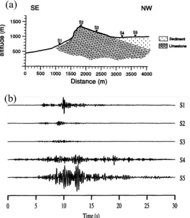
After the earthquake occurred on 26 September 1997 in central Italy, the historic center of Nocera Umbra, lying on top of a 120 m high hill, was found diffusely damaged. Some recently built houses even suffered a higher level of damage on the top of the hill, where the marly limestone of the ‘Scaglia’ formation crops out. Caserta et al., (2000) investigated the possible correlation between ground motion amplifications and the observed seismic damages. Five portable stations were deployed in eight sites along a 2.5 km profile to record the aftershocks (Figure 1.9). They analyzed the ground motion with different methods: the classical spectral ratios and the horizontal to vertical spectral ratios calculated both on noise and earthquake data. Amplifications of 2 to 3 at a frequency range of 2.5-5 Hz were obtained at the top of the hill. In the frequency band around 20 Hz, an extremely high value of amplification of 20 for the standard spectral ratio was observed at station 5 at the middle of the ridge. However, at frequencies lower than 10 Hz, the high amplification was obtained at stations 1 and 2

(27)

located on a flat site. This suggests that the near-surface geological layers are probably responsible for the observed amplifications.

Figure 1.9: The portable stations installed along the ridge and the spectral ratios derived for several sites. The results

show that high ground motion amplif ication is likely to be attributed to the near -surface geology. Legend defines: a) Recent alluvium; b)‘Marnoso-Arenacea’ formation; c) ‘Scaglia’ formation; d) faults; e) seismic stations. (Caserta et al., 2000).

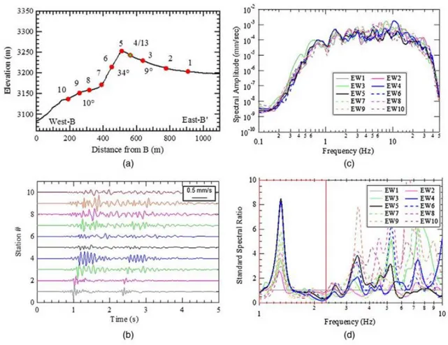
Buech et al. (2010) deployed seven seismometers along a ridge, which is a 210 m high, 500 m wide, and 800 m long hill (Figure 1.10). Seismic records of local and regional earthquakes were recorded and analyzed using three methods: comparisons of the recorded peak ground accelerations, power spectral density analysis, and standard spectral ratio analysis. Both time and frequency domain analyses show that high topographic amplifications occurred along the ridge with respect to the reference motion recorded at the station rh0 located on the flat base and the maximum amplification ratio in the frequency domain at station rh6 can reach 11. The spectral ratios show that a maximum response occurred for frequencies of about 5 Hz (Figure 1.11).

(28)

Figure 1.10: Arrangement of the array in the study area. (a) Location of the epicenter; (b) topographic map; (c) the

profile showing the distribution of the seismometers (Buech et al., 2010).

Figure 1.11: The spectral amplitude of the observed ground motions for two horizontal components. The results

(29)

Severe building destructions during the 2011 February Mw 6.2 and the June Mw 6.0 Canterbury

earthquake (New Zealand) were considered to be caused by topographic effects, because damage patterns suggested that ground motion amplifications due to localized features have likely been responsible for the most severe effects (Kaiser et al., 2013). To evaluate the site effects on ground motion amplifications, temporary arrays were deployed at four sites. The ground motions were collected from aftershocks in order to characterize the seismic site response and to assess amplification from lithological and topographic factors. The initial analyses from records at two of the sites suggested significant complexity in ground motion amplification and revealed polarization over small distances within the arrays for any given event.

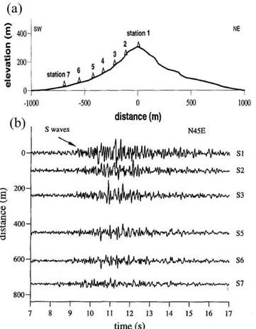
In 2003, dense arrays of seismometers were deployed at a steep mountainous terrain in Central-Eastern Utah (USA) in two directions with varying slope angles and topographic features (Figure 1.12) to record ground motions and thus to assess site effect on ground motion amplification (Wood, 2013). The researcher analyzed the ground motions recorded at the mountainous site and assessed changes of the frequency content and amplitude of available ground motions affected by topographic features. The results show that the instrumented peak ground motions were affected in a narrow frequency range by the effects of topography (Figure 1.13). It is also clear that the physical phenomenon of topographic effects was not only observed at the crest of the slope, but also along the slope and at the base of the slope. The highest amplification factors were produced at the crest of the slope while amplifications decreased downwards along the slope. At the toe of the slope, deamplification occurred.

Figure 1.12: The location of seismic stations used during Phase I of recording (N-S and E-W cross-sectional profiles

(30)

Figure 1.13: Examples of results from Event 17801 Phase I, Stations 1–10, E-W component: (a) E-W topographic

cross section, (b) time records, (c) Fourier amplitude spectra, and (d) standard spectral ratio (Station 1 used as the reference station). Expected topographic frequencies based on simple analytical formulas range from 0.79–2.39 Hz, as indicated by the inset box in (d) (Wood, 2013).

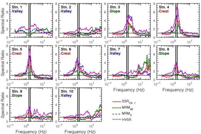
Recently, an experimental study, investigating potential topographic amplifications of ground motion, was carried out on a soft rock ridge of a height of 50 m, which is located at Los Alamos National Laboratory, New Mexico (Stolte et al., 2017). Seismic arrays of ten portable broadband seismograph stations were deployed across the ridge for monitoring ambient vibration data during 9 hours. By comparing spectral ratios of ambient noise recordings, clear evidence of topographic amplification was obtained at the slope crest of the instrumented ridge. The predominant frequency of the ridge observed from the spectra of experimental recordings is in agreement with the theoretical estimation based on its geological and geometrical features. The results suggest that ambient vibrations monitoring is a feasible way to quantify the frequency range of topographic amplifications. Spectral analyses by using standard spectral ratio, median reference method, and horizontal to vertical spectral ratio, were performed to quantify topographic effects, as well as to make comparisons. A topographic map can be seen in Figure 1.14 and a comparison of spectral ratios is illustrated in Figure1.15.

(31)

Figure 1.14: Topographic map of the instrumented ridge, showing the location of seismic stations 1–10. Cross

section A–A′ showing the location of seismic stations placed along a line parallel to the direction of elongation of the ridge. Cross section B–B′ showing the location of seismic stations placed along a line perpendicular to the direction of elongation of the ridge (Stolte et al., 2017).

Figure 1.15: A comparison of the spectral ratio in the horizontal direction perpendicular to the axis of elongation of

(32)

1.2.1.2 Theoretical analyses

Volume waves (P, S) and surface waves (Rayleigh, Love) involved in a seismic event can be generated or transformed when earthquake waves travel through a medium with geological irregularity or at the surface of the earth due to wave interferences, reflections and diffractions. Simplified theoretical equations are often used to evaluate topographic effects on wave transmission near the ground surface at a given site. Using these simplified methods, simple homogeneous 1D or 2D problems are often studied when subjected to vertically propagated SV waves or sometimes SH waves. However, under certain circumstances, these analyses can quickly provide a good approximation that can be applied to deal with real engineering situations and thus are welcome to solve engineering problems. A review of the most widely used theoretical methods to evaluate ground motion amplification due to topographic features is presented hereafter.

In 1960, Ambraseys presented a theoretical study for analyzing the shear response of a truncated 2D elastic wedge subjected to an arbitrary disturbance (Ambraseys, 1960). Elastic and constant rigidity of the wedge is assumed, and only shear movement along the wedge faces was considered for the equation derivation. He derived equations to estimate the response in shear of the wedge-shaped elastic solid, which is verified to be suitable to earthquake engineering problems, in particular to those dealing with the seismic stability of earth dams and embankments.

Shortly afterwards, Gilbert and Knopoff developed a perturbation solution for 2D elastic geometry, in particular for the case of irregularities with gentle curvature (Gilbert and Knopoff, 1960). The approximation is based on the assumptions of small magnitude and slope of the irregularity. The irregularity is replaced by an equivalent stress distribution. This method was used by Hudson for a case study of a small slope. By analyses using this approach, results with respect to Rayleigh waves are found to be in good agreement with observations, even for topographic irregularities characterized by slope angles greater than 25° or 30°(Hudson and Boore, 1980).

Because the conversion mode of SH waves is simpler than the generation of P, SV or Rayleigh waves, researchers have mainly studied the wave propagations due to topographic effect using incident SH waves. Trifunac (1971) investigated a semi-cylindrical alluvial valley for characterizing surface motion in case of incident plane SH waves. He showed that the complex phenomena of wave- interferences are characterized by wave patterns and rapid changes in the ground- motion amplification are observed along the free surfaces. These phenomena depend on the incidence angle of SH waves. Then, Wong and Trifunac (1974) performed another analysis on a semi-elliptical canyon to examine the dependency of ground motion amplifications on the surface and near the canyon. The results suggest that the amplification ratios depe nd on the incident angle of the input motion and on the ratio between the width of the canyon and the wavelength of SH waves.

At the meantime, Aki-Larner method (Aki and Larner, 1970) was developed and applied to a study of the seismic response of sediment- filled valleys subjected to SH waves (Bard and Bouchon, 1980). The results confirmed that the Aki-Larner technique is a powerful and reliable tool to study scattering effects of earthquake waves in the time domain, in particular when wavelengths of the input motion are comparable to the size of the structural feature. They also demonstrated that a non-planar interface has a great effect on ground motion amplifications due to the generated Love waves which were observed to have much larger amplitudes than those of input motion. Moreover, the duration of the ground shaking in the basin was much longer due to the presence of a high-velocity contrast between the surface layer and bedrock.

(33)

In 1985, Sánchez-Sesma (1985) derived and applied Macdonald's solution to study the diffraction of SH waves propagating in a wedge-shaped elastic medium. It was observed that the motion near the wedge was substantially affected by the wedge angle. Paolucci (2002) estimated the fundamental frequency of homogeneous triangular mountains using the Rayleigh’s method and then evaluated topographic amplification on this relief by the spectral element method. The results show that topographic irregularities with significant elongations are like to induce wide-band frequency amplifications while isolated cliffs are responsible for amplifications at a narrow range of frequency. Later, Smerzini et al. (2009) presented several analytical methods based on the expansion of Bessel and Hankel wave functions in order to study the anti-plane seismic response of various types of underground structures. Moreover, they also applied the Rayleigh’s method to verify that the ground motion amplification was dominated by the fundamental resonance frequency of soil profile.

1.2.1.3 Numerical modeling

Numerical modeling analysis has been widely developed to predict ground motion modifications due to topographic effects. 1D, 2D and more recently 3D numerical simulation, for various steep reliefs such as slopes, ridges, cliffs, and mountains, have been carried out for assessing topographic effects on ground motion (Assimaki et al., 2005; Geli et al., 1988). Thank to the development of computer technology with the updates of software, more and more complex models have been designed. These research works used the finite difference method (Lenti and Martino, 2012; Zahradník and Urban, 1984), the finite element method (Assimaki et al., 2005), the boundary method (Sánchez-Sesma et al., 1982), the discrete wavenumber method (Bouchon, 1973), and the Aki- Larner method (Geli et al., 1988; Wong and Jennings, 1975). Below is a review of studies that have been performed using numerical modeling.

In 1972, Boore carried out finite difference calculations to analyze the propagation of SH wave in a step-like slope. The results show that topography plays an important role in seismic wave propagation, especially when the wavelengths are comparable to the characteristic model size like slope height (Boore, 1972). It also showed that ground motion changes due to topographic effect vary from amplification to deamplification depending on the frequency contents of the input motion. Ground motion amplifications can reach 75% compared to the motions observed at a site without the effect of topography. Later, Boore (1973) conducted calculations for simple geometrical models and compared the results with observed data near Pacoima Dam during 1971, February 9th, San Fernando earthquake. The results suggest that topography has a large influence on ground motion recorded on the ground surface. The ground motion amplification is significantly frequency-dependent, and the amplification ratio for higher frequency excitation can reach 1.5 times as much as those results due to lower- frequency input motion. Afterwards, numerical investigations of topographic effects on slope model subjected to vertically incident SV waves and P waves were performed using the finite difference method (Boore et al., 1981). The results indicated that scattered Rayleigh waves were considered to be mainly responsible for causing ground motion amplifications. The amplitudes of Rayleigh waves can be as large as 0.4 times the amplitude of the incident waves.

In 1973, Bouchon performed a parametric study on topographic effects using the Aki and Larner method in order to investigate the effect of topography on the surface motion in the cases of incident SH, P and SV waves (Bouchon, 1973). In the numerical simulations, the variation of the topography, the incident angle of input motion, and wavelength of seismic waves were considered. Results showed that the surface topography has a great influence on surface displacement. In the case of a ridge,

(34)

ground motion amplification is observed near the top, while deamplification occurs near the bottom. For a case study of the Pacoima Dam, the high accelerations recorded during the San Fernando earthquake are supposed to be amplified by a ratio of 1.5 due to the effect of topography.

Later, Bard used the Aki-Larner technique to conduct a numerical study aimed at investigating the respective influences of surface geometry, elastic parameters and incident wave characteristics on ground motion (Bard, 1982). The topographic effects are found to be extremely depended on the incident wave characteristics and expressed a great complexity. When the wavelength of the incident waves is similar or slightly shorter than the mountain width, ground motion amplification occurred systematically. It is also showed that the complex wave scattering is frequency-dependent and is likely to be closely correlated to the horizontal scale of the topographic structure. Moreover, higher ground motion amplification was observed for incident S waves than for P waves.

In 1983, Ohtsuki & Harumi numerically studied the effect of topography and surface geology on the ground motion. Numerical simulations were made for several types of topography, such as a cliff, a cliff with a soft layer and filled land, using finite element method (Ohtsuki and Harumi, 1983). Their study demonstrated that displacements recorded on the surface are very much influenced by topography, in particular when the incident wavelengths are comparable to the size of the topographic features. Rayleigh waves are generated at the slope toe and slope crest. They also s uggested that the amplitude of Rayleigh waves recorded behind the crest can be 35% higher than the amplitude of the incident waves at the free field surface.

Afterwards, the finite-difference method is applied to simulate elastic wave propagation through a 3-D model of the Santa Clara Valley (Frankel and Vidale, 1992). The numerical model (30 (east-west) × 22 (north-south) × 6 (depth) km) corresponded to a large mountain area and was divided into many zones with 4 million grid points. A synthetic motion from a magnitude 4.4 corresponding to the aftershock of the Loma Prieta earthquake was used as input motion. The numerical simulations confirmed topographic amplifications and showed how S waves are converted to surface waves at the edge of the basin. It is observed that Love waves produced at the edge of the basin are the largest arrivals of the transverse waves and Rayleigh waves are produced along the southern margin of the basin. In addition, 2-D simulations were also conducted to analyze the effects of the wave incident angle and impedance on wave conversion at the basin. In another study, Frankel showed that the synthetic seismograms from 3D simulations have a larger amplitude than those derived from a 2D model (Frankel, 1993). Moreover, he simulated the San Andreas Fault to demonstrate how the rupture directivity affects the pattern of maximum ground motions on the surface of the basin. It was concluded that the presence of off-azimuth surface wave arrivals increased the ground motion amplitude in the 3D simulations and these off-azimuth arrivals represent surface waves produced at the edges of the basin.