Strategic Interactions between Monetary and Fiscal
Policies: a case study for the European Stability Pact
Jerome CREEL #*
Abstract: We extend the model of Leith and Wren-Lewis (2000) to the case of a monetary union. Within a two-country dynamic model with wealth private behaviours, we study the implications of stabilising public debt on monetary and fiscal policies. The model is a macroeconomic version of the Fiscal Theory of the Price Level. We introduce an asymmetry in fiscal policies: one fiscal policy is ‘active’ in the short run; the other is always ‘passive’. Both policies are the outcomes of a game between the two governments and the ECB. In this framework, we assess the ‘beggar-thy-neighbour’ consequences of the passive fiscal policy in the fiscally-constrained country. Because of the inability of this government to implement an ‘active’ policy, the other government may incur a higher public debt burden. The ECB has to get more involved in the macroeconomic stabilisation process and has to prevent fiscal policy in the country with sound public finance from being too much active. The more substantial these ‘beggar-thy-neighbour’ effects, the more profitable cooperation between governments and the central bank.
JEL Classification: E17, E63, H63
Keywords: monetary and fiscal policies, fiscal theory of the price level, EMU, Stability Pact.
#
OFCE and CREFED (U. Paris-Dauphine, France); address: OFCE, 69, Quai d’Orsay, 75340 Paris cedex 07, France; tel.: (33) (1) 44 18 54 56; fax.: (33) (1) 44 18 54 78; email: [email protected].
*
This is a revised version of a paper presented at the 2001 Royal Economic Society Conference held at the University of Durham. I gratefully acknowledge Campbell Leith for providing me with very helpful and comprehensive comments. My thanks also go to João Amador, Patrick Minford and Matthias Sutter for their remarks. A preliminary and quite different version of this paper has been presented under the title: “The Stability Pact and Feedback Policy Effects” at the 16th Journées Internationales d’Economie
Monétaire et Bancaire, Poitiers, june 1999, and at the Money, Macro and Finance Conference, London, september 2000. I do thank participants for their remarks. The usual disclaimer applies.
1. Introduction
In a recent paper, Leith & Wren-Lewis (2000) – hereafter LWL - examined the interactions between monetary and fiscal policy in a closed economy with sticky prices and non-Ricardian consumers (finitely-lived agents face a higher discount factor than the government). These deviations from the neo-classical framework implied a richer set of interactions between policies than the usual channel of seigniorage revenues or surprise inflation at the core of the Fiscal Theory of the Price Level (FTPL). LWL demonstrated that two stable policy regimes could be identified: in the first one, monetary policy would be ‘active’ in the sense determined by Leeper (1991), i.e. reacting toughly to inflation deviations from their steady-state value; while fiscal policy would be ‘passive’, i.e. reacting toughly to public debt deviations from their steady-state value. In the second one, monetary policy’s reactions towards inflation would be smoother whereas the government would stabilise public debt very slowly. This case was clearly the closest to Woodford’s work (2000) dealing with the FTPL.
This theory states that the price level can be determined through the satisfaction of the intertemporal government budget constraint. It implies that a government can exogenously fix its real spending and revenue plans, and that the price level will take on the value required to adjust the real value of its contractual nominal debt obligations to ensure government solvency. The mechanism underlying the FTPL is linked to a wealth effect (Woodford, 2000): if the sequence of future primary fiscal deficits entails an increase in the contractual nominal debt obligations of the government, households will feel wealthier and will consume more, so that the general price level will be increased insofar as the government budget constraint is satisfied1. Contrary to what Buiter (2000) said about this constraint, it is not used as an “equilibrium condition” in the FTPL, and is therefore valid for all possible values of the price level and output.
The FTPL has already been extended to the case of a monetary union (Woodford, 1996, Bergin, 2000), but within a neo-classical framework and without nominal inertia in the price setting in the short run. Moreover, net external assets were not part of the story, although they may help the stabilisation process of both economies after a shock. Last, there was no insight concerning the structure of stable fiscal and monetary rules.
We extend LWL model to the case of two countries engaged in a monetary union and in considering optimal policies as the outcome of a game between two fiscal authorities and a single monetary policy, implemented by the European Central Bank (ECB). We specifically study the implications of the Stability and Growth Pact, i.e. the possibility that one country could be unable to react to a shock because it has no fiscal room for manœuvre, whereas the other country could implement a fiscal policy to stabilise the economy2. Such an asymmetry in fiscal policy rules is not unlikely in the
1
“Equilibrium is restored when prices rise to the point that the real value of (the nominal liabilities of the government) no longer exceeds the present value of expected future primary surpluses, since at this point the (private plus public) expenditure that households can afford is exactly equal in value to what the economy can produce.” (Woodford, 2000, p.18)
2
Indeed, the Stability and Growth Pact prevents countries in the Euro area from increasing public deficits over 3% of their GDP, except in the case of a substantial slump. Countries which would not satisfy the Pact may incur fines (cf. Beetsma & Uhlig, 1999, for a stylised rationale of this Pact). As fines may be long to come (the process under which European countries may order the fine lasts two years), the
Euro area. Though the ratios of public deficits are less dramatic than in the early nineties and though the Maastricht’s norm on public debt has been wiped out as regards the entry of some countries in the Euro area, the public finances in these countries (Belgium, Italy and Greece) are still carefully supervised by the Commission, via the Stability and Growth Pact, or by the ECB before it sets the European nominal interest rate.
A situation with asymmetric fiscal framework between two countries forming a monetary union could have strong feedback policy effects on the implementation of monetary and fiscal policies. The country whose fiscal policy would be aimed at stabilising the economy could suffer from its interdependence with the other country: a negative shock in the latter country could provoke a higher public debt in the first country; and this would impede its future capacities to implement an active fiscal policy3. The ECB, in its goal of “price stability”, would not be immune either against the consequences of fiscal policies, as stated in LWL. For instance, if a negative shock occurred in the country which cannot react through its fiscal policy, the ECB would increase the nominal European interest rate. Hence, it would have to “substitute” for the absence of fiscal policy in the country under the rule of the Pact. In the long run, if households have a wealth effect linked to public debt, the ECB would have to adjust households’ private wealth plans to actual public debt and net foreign assets levels: if, for example, public debt increases in relation to GDP, the ECB would have to choose between reducing the interest rate to curb debt’s accumulation or increasing it to make private wealth grow faster. Depending on their reactions in the long run, the ECB and the governments would be fettered in the timing as well as the scope of their policy choices, and their ability to smooth economic fluctuations might well be affected by the constraints of the Pact (see also Hughes Hallett & Vines, 1993, and Jensen, 1997).
The paper is structured as follows. In section 2, we present LWL model briefly. In section 3, we outline our analytical framework, stressing its most notable features. Section 4 provides an assessment of the consequences of supply and demand shocks in the monetary union, whether symmetric or asymmetric. The shocks in the economy (or economies) are supposed to be permanent. For each shock, we study the Nash equilibrium between the three policy makers and then compare it to a cooperative equilibrium which we computed according to the Nash-bargaining procedure. Section 5 stresses the most substantial costs emerging from the implementation of the dispositions of the Stability and Growth Pact. Section 6 finally brings out some conclusions.
2. Leith & Wren-Lewis model
LWL examined the extent to which central bankers need to be concerned about what fiscal policy makers are doing. They looked at a closed economy in which the central bank implements a simple rule that raises interest rates if inflation is above target, and the government adjusts its spending or taxes to meet a target for government debt.
SGP may not appear ‘credible’. In the following, we however consider that the SGP is so credible as to be satisfied by any country over the deficit limit.
3
Note that, contrary to “mainstream literature” (see, for instance, Chari & Kehoe, 1998), debt monetisation is not part of the story. This is probably on this point that the FTPL is the most attractive.
LWL (2000) showed that independent central banks cannot ignore what the government is doing with fiscal policy. However, as long as stabilisation of government debt is sufficiently passive, central bankers can raise the real interest rates by as much as they want in order to hit their inflation targets. The direct implication of this process is that while fiscal policy must react to some extent to variations in government debt, their response needs not be dramatic. Stated briefly, this does not seem to legitimate the tight control of fiscal policy implied by the European Stability Pact.
The model of LWL originates in the Blanchard (1985) perpetual youth model: since households face a finite life, they consider (a part of) public debt as net wealth. Aggregate demand thus depends positively on public debt and public spending, negatively on taxation:
t t t t
Y =kB −cT +G , where B represents public debt, T taxation, G public spending and parameters ‘k’ and ‘c’ are positive.
The Phillips curve is such that:
t aYt
•
π = , where •
π is the inflation rate in difference.
With parameter ‘a’ negative, this equation is simply a forward-looking Phillips curve. Be ‘a’ be positive, and one obtains a traditional backward-looking Phillips curve. It is quite interesting to note, first, that conditions for stability are in no way dependent on the assumption concerning parameter ‘a’4. Second, inflation dynamics is quite different whether you introduce adaptive or rational expectations. If ‘a’ is positive (adaptive expectations), a GDP reduction provokes a linear decrease in inflation. If ‘a’ is negative (rational expectations), inflation is deeply reduced and then progressively rises to its new steady-state value. In the following, we will hinge on Fuhrer (1997) and favour adaptive expectations as our specification for inflation dynamics.
LWL consider two specifications for fiscal policy. If the government stabilises public debt via public spending, its framework is of the following form:
[Case 1] Gt G f[Bt B]
− −
= + − , and Tt = τYt,
where τ is the tax rate, a superscript is a target value, and a subscript is time. Government spending responds to public debt deviations from the target and taxation is applied at a constant rate.
The alternative fiscal framework is of the form:
[Case 2] Tt = +T f[B− t−B]− and Gt =G− . The government adjusts taxation to meet its public debt target; government spending is assumed to be constant5.
On empirical grounds (see the seminal paper by Alesina & Perotti, 1995), one should favour case 1 for the fiscal framework. It has been demonstrated that fiscal adjustments were in fact more efficient when expenditures had been reduced, rather than
4
If ‘a’ is positive, there are two pre-determined variables in the model (wealth and inflation); and if ‘a’ is negative, only wealth is a pre-determined variable. In the first case, the determinant of the system of dynamic equations must be positive; but negative in the second case. Since ‘a’ enters as a common factor in the determinant, its sign does not modify necessary conditions for stability.
5
taxation increased. LWL also favour case 1 in their numerical simulations. Reason for this is the little influence of taxation on output and inflation, a situation which denies any substantial fiscal feedbacks on the optimal monetary policy (LWL, p.C101). Adding a second country automatically increases the fiscal feedbacks on monetary policy, via the fiscal policy of the second country and, thus, tends to limit the above argument by LWL. In the model we will use below, using either a modified version of case 1 or a modified version of case 2 gives the same kind of results6.
In their conclusion, LWL state that, if fiscal policy is relatively active in Leeper’s sense – debt is stabilised very slowly, whatever the case for fiscal policy is chosen –, then this puts severe constraints on what monetary policy can do. If monetary policy responds to excess inflation by raising real interest rates, this will lead to destabilising movements in output as government debt “explodes”. However, as long as fiscal policy is sufficiently passive, central bankers are free to raise real interest rates by as much as they want. The implication is that one needs to ensure that fiscal policy responds to some extent to changes in government debt, but this response needs not be as tough as what the Stability Pact seems to generate.
In the following, we concentrate on the implications of policy rules interactions in the open economy and, more explicitly, in a monetary union. Consumers therefore hold their wealth not only in the form of public debt, but also in the form of external assets. In such a situation, within a monetary union, i.e. in the absence of any exchange rate risk, a target for public debt is needed in order to determine the allocation of wealth between net foreign assets and public debt. This is another reason for discussing the degree of relevance of fiscal policy rules. Without a target on public debt, wealth could well be balanced with unstable and symmetric levels of public debt and external assets7.
3. Some extensions to the previous model
We do simplify LWL model in two respects, with minor consequences on their results: we do not take human wealth nor money into account. The latter exclusion is studied in LWL model. Finally, we extend it in five respects. Three are linked to the open economy and policy rules: we introduce two countries and a common central bank (which we call the ECB); we consider an asymmetry in the fiscal framework between the two governments; and their policy rules are the outcomes of a game between the two governments and the ECB. The two other assumptions deal with consumption: we introduce a wealth effect which resembles the Pigouvian “real balance” effect; and a non-linear effect of the real interest rate on aggregate demand is included.
3.1 The general framework
The model drops the Blanchard specification of intertemporal consumption and replaces it with a specification where (still non-Ricardian) consumers consume their
6
In our model, in cases 1 and 2, the tax rate and public spending in each country are set respectively as the outcome of a game between the two governments and the ECB.
7
In a flexible exchange rate regime or in the EMS, the uncertainty regarding the future value of external assets denominated in foreign currencies or the risk aversion by households are sufficient conditions for determining the discrepancy between domestic and foreign assets.
current income (including interests received on net financial wealth), plus a proportion of their financial wealth. The model has thus Keynesian features in the short run (output is driven by the level of demand, prices adjust slowly to their steady-state levels) but Wicksellian features in the long run: output is determined according to the real equilibrium interest rate, which depends on the effects of monetary and fiscal policies on the inflation rate. Aggregate supply follows a Phillips curve.
We study a polar case in the EMU: two countries, identical as far as private behaviours are concerned, form a monetary union8. Households in both countries hold their wealth under the form of domestic public debt (D) and net foreign assets (F).
In the Blanchard (1985) model, the aggregate consumption function C was shown to be:
t t
C = + σ(k )D , where k is a constant probability of death and σ is the discount rate. The real interest rate does not appear directly in consumption, nor in aggregate demand – there is no capital in the economy – but, indirectly, it has two effects: higher interest rates reduce discounted human wealth leading to a fall in consumption, but as net financial assets increase, consumption increases also.
We keep this non-linear effect in the following, but without any human wealth. The real interest rate has theoretically two opposite effects on aggregate consumption in the short run if the net asset position is positive: substitution and wealth effects. Noting W the private wealth, we assume in the following that the former effect dominates the latter: private savings increases, i.e. the part of net disposable income which is devoted to the accumulation of wealth increases, and consumption decreases. In the long run however, we go back to the usual net wealth effect: wealth increases with the real interest rate and consumption is higher. Aggregate demand will hence depend negatively on the real interest rate in the short run, and positively in the long run.
To obtain this result, we use the formulation adopted by Tobin and Buiter (1976) and according to which savings is regarded as a process which adjusts wealth towards some target value relative to income. We therefore consider that private agents form wealth plans W
∼
which positively depend on disposable income net of wealth interests ( (1− τ)Y), but also on the real interest rate (ρ)9:
(1a) Wt = α + βρ( t)(1− τt)Yt ∼
, where β represents the sensitivity of the private wealth effect towards the real interest rate. For a zero real interest rate, the wealth over disposable income ratio is supposed to be positive (α is positive).
If actual real wealth differs from planned wealth, households behaviour makes it adjust to its desired level at speed µ. The demand block of the model is therefore given by a somewhat usual IS curve:
(1b) Yt = − τ(1 t)Yt+ ρtWt + µ[Wt−W ]t + η(Y * Y )t − t + ηε π −π +( t* t) Gt+Xt ∼
.
8
Asymmetric private interdependence between the two countries (for instance, different pace of adjustment for prices or wages after a shock, as in Hughes Hallett, 1986) are not dealt with in the present paper.
9
Aggregate demand increases with disposable income, plus interests on wealth ( Wρ ), with the gap between actual and planned wealth, with public spending (G) and with a private demand shock (X). The additional terms in output and inflation differentials reflect spillovers from the second country through the trade balance. The ε parameter represents the elasticity of the trade balance to the variations of the inflation differential, it is positive; η is the degree of openness.
Including equation (1a) into (1b) gives a negative effect of the real interest rate on aggregate demand in the short run insofar as W− µβ − τ(1 )Y<0 at the steady state, and a positive effect in the long run insofar as W>0. Both conditions are met within our parametrisation.
The wealth effect introduced in the aggregate demand is close to the Pigouvian or “real balance” effect: if actual wealth is beneath its planned level, because of an increase in the real interest rate, private consumption will be reduced until savings has reached the desired equilibrium level. In the long run, households will use this savings in order to boost their own consumption.
Aggregate supply is derived according to a Phillips curve in the open economy. Real wages are indexed on the consumer price index (inputs are not imported),
(2) π = π + λ + η π −π +t t 1− Yt ( t* t) zt, where z is a supply shock.
Expectations are assumed to be adaptive (cf. section 2, parameter λ is positive). We concentrate on the interactions between fiscal and monetary policies only, without any interference with a fourth player, namely households. Assuming adaptive expectations, we can neglect this fourth player while in the meantime being assured that in the long run, inflationary expectations will be met (see Blake and Weale, 1998). Another way to motivate the adaptive expectations assumption would be to argue that the private sector may act adaptively during the early stages of Monetary Union as they learn more about the new policy regime.
Wealth (equation 3) is the sum of public debt and net foreign assets which grow after a trade deficit:
(3) Wt =Dt +Ft.
Equations (4) and (5) describe the dynamics of these two assets: (4) Dt = + ρ(1 t)Dt 1− +Gt− τtYt;
(5) Ft = + ρ(1 t)Ft 1− + η(Y * Y )t − t + ηε π −π( t* t).
The model is supposed to be quarterly. Shocks occur in the first quarter of 2000 and are permanent.
3.3 Governments and the ECB
The two countries, named respectively A and B, are engaged in a monetary union and consequently share a common currency. The common central bank (which we will call the ECB) implements the monetary policy in the union. The rest of the world is neglected. The fiscal policy framework is asymmetric.
3.3.1 Government A
Government A uses its tax rate to minimise its loss function (equation 6) each year so that its policies are strategic, rather than ad hoc as in LWL10. The quadratic loss function depends on the differences between respectively, output, inflation, tax rate and public debt, on the one hand; and their initial steady-state values, on the other. Public debt is expressed in percent of the GDP.
(6) LGt = ∆a0 Y ²t + ∆π + ∆τ + ∆a1 t² a2 t² a3 (D / Y )²t t .
Parameters a0, a1, a2 and a3 are positive weights on respective targets. Targets for
output and inflation are uncontroversial. We also assume that the loss function includes a term which captures the costs of tax collection (see Barro, 1979). In country A, the government has to stabilise public debt over GDP, at least in the long run. Many arguments are here worth mentioning. First, this is in line with LWL’s conclusions. Second, via the net wealth effect, higher debt fuels aggregate demand and inflation and is thus detrimental to the first two targets. Limiting the debt to GDP ratio should permit a better allocation of the fiscal instrument to output and inflation targets. Third, it also permits to include a kind of intertemporal mechanism in our static game approach: the loss function is minimised at each period, but since it incorporates debt accumulation, the government implements a trade off between satisfying its first two targets, on the one hand, and the consequences of its actions on its future rooms for maneuver (public debt as a proportion of GDP), on the other hand.
3.3.2 Government B
Despite the Stability Pact, it is not at all sure that countries in the Euro area will be fettered by its provisions after a shock. This will be all the more true if they have already recovered fiscal room for manœuvre. However, some countries will surely have to spare any additional increase in their public debt over GDP ratio in the following years. These countries will have to pursue balanced-budget rules in the best case, or to keep on reducing their deficits, in the worst.
In the following, we assume that country B is in the situation of being constrained by the Pact. It has to follow a fiscal rule which will keep public deficits in line with the stability of the debt to GDP ratio. We assume that it has already reached the ceiling of the Pact, considered here as the steady state level of the public debt ratio. As stated earlier, we will favour case 1 (see section 2) for fiscal instruments. Public spending, rather than taxes, are set in order to stabilise public debt (in GDP share). We introduce a lag in government spending, which represents the relative inertia of expenditures. Moreover, government B is able to use its tax rate τ to minimise the same loss function as government A:
(7) LG *t = ∆a0 Y * ²t + ∆πa1 t* ²+ ∆τa2 t* ²+ ∆a3 (D * / Y *)²t t ;
(8) G *t = − χ(1 )Gt 1− *+χ τ[ * Y *t t −ρtD *t +µ Φ −g( D *)]t .
10
In order to simplify notations, we did not add an intertemporal discount rate in the loss functions. We do not intend to compare losses from one period to the other but, rather, at a certain time, from one equilibrium (Nash) to the other (cooperation). Time-consistent equilibrium is beyond the scope of this paper.
The Φ letter represents the public debt target of government B; it is exogenous. The
χ
µg parameter represents the speed of adjustment of the public deficit to the level
required to reach Φ. In order for stability conditions of the model to hold, this speed has to be high.
The fiscal framework for government B is a bit more complicated than case 1 in LWL, because both fiscal instruments (tax rate and public spending) are endogenous: one is set as the outcome of a game with the other authorities, whereas the other is set according to a feedback rule which is set such that the primary fiscal deficit remains under control.
The introduction of two equations in the fiscal framework of government B aims at three objectives, plus that of being as close as possible to LWL formulation. First, we compute Nash-bargaining equilibria to assess the gains from cooperation; we thus need a loss function of type (7). Second, the cost of tax collection is not sufficient to limit fiscal policy toughly in the short run, so that we need equation (8) which is more stringent. Third, macroeconomic models in the EMU usually use equation (8) as the sole strategic behaviour of governments11; but we found interesting to shed light on the differences between the results obtained via equation (8) with that obtained via the policy design for government A (equation 6).
Of course, the fact that government B controls two instruments (rather than one for government A12) and has the same number of targets as government A should not lead to the conclusion that the “constrained” authority is freer than government A13. In our short-run Keynesian framework, a limit on public deficit is a strong constraint for a government as far as the stabilisation of output and inflation to their respective steady states is concerned.
3.3.3. The ECB
The monetary union is characterised by the uniqueness of the nominal short run interest rate (i) and the independence of the ECB. We assume that the ECB implements its monetary policy through the setting of this nominal rate. We avoid the difficulties regarding the definition and level of money supply in a monetary union and the complications due to the instability of money demand in financial economies. The ECB minimises the average and squared deviations of inflation from its target and the average and squared deviations of output from the steady state:
(9) t t t t t 0 1 2 t ,M Y Y * * LM k ( )² k ( )² k ² 2 2 + π + π
= ∆ + ∆ + ∆ρ , where the average real
interest rate is t t t,M t * i 2 π + π ρ = − .
The ECB is supposed to be reluctant to deviate the real interest rate from the steady state. In our macroeconomic framework, this can be justified on four grounds. First, too large deviations of the real interest rate have costly effects on the patrimonial
11
See Barrel & Sefton (1997), Capoen & Villa (1997), Jensen & Jensen (1995), van der Ploeg (1995).
12
Actual public spending in country A is supposed to be constant and set equal to a target level, GA. 13
equilibrium: if the real interest rate soars in the short run, this will provoke a steep increase in public debt in both countries, unless government A increases its tax rate dramatically and government B decreases its public spending sharply. Both moves in fiscal policy are costly for the governments, but they are also for the ECB: they reduce the future capacity of governments to stabilise output and inflation, so that the burden of future shocks might fall on the central bank. If governments do not react to the initial increase in the real interest rate, the ECB might have to decrease the rate to stop debt growth (its initial policy would therefore have been useless), or might have to increase it further to compel governments to contract their deficits: the conflict arising between the ECB and governments might lead to excessive rises in the real interest rate and public deficits. Second, the reluctance of the ECB can be thought of as representing inertia in policy making14. More generally, the reluctance of the ECB towards too large variations in the real interest rate could be justified by the ECB’s concern for a stable aggregate private investment. Or, the ECB may want to prevent the banking system from being weakened by frequent and large swings in the discount rate which they would have to pass on to their customers.
Macroeconomic models usually give the priority to inflation in the central bank loss function, according to the “credibility” argument: the government inflation bias needs a tough reaction by Central bankers. Although our model does not bear on such imperfections as the inflation bias, we ensure that our specifications for fiscal and monetary policies do not depart on this point from the mainstream literature. With no costs for the use of fiscal or monetary instruments, k1 should have been therefore
superior to k0 and (k1/k0) should have been superior to (a1/a0). In our formulation with
costs, this latter condition can be rewritten as:
(10) (k1−k ) / k2 0 >a /(a1 0+ −a2 a )3 , since the cost of using the interest rate reduces
the capacity of the ECB to curb inflation, and the cost of using the tax rate and the cost of increasing public debt reduce the capacity of governments to stabilise output. We will ensure that parameters verify this condition.
3.4. Parameters
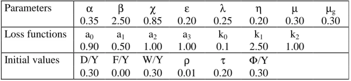
Since analytical solutions of the model in the face of shocks are intractable, we set the model in deviation from the steady-state and we adopted a parameter set in order to study the dynamic paths of model variables following the shocks. Our central parameter set is given in table 1. We chose some of them so that fiscal and monetary short-term multipliers match those of the macroeconometric international model MIMOSA (see Le Bihan & Lerais, 1998).
Output is normalised at unity, and steady-state government spending is 19.7% of GDP, hence the amount of funds for net expenditures in the general budget of France in 1999. Initial public debt is equal to 30% of GDP and corresponds to net public debt in France in 1994, thus before the cyclical increase in public deficits at the beginning of the nineties had been converted in public debt. The real equilibrium interest rate is 1% and corresponds to the gap between the interest rate and the GDP growth rate in France in 1999.
14
The same argument applies to the presence of the tax rate in the loss functions of both governments.
Table 1: Parameters and Steady-State Values of Variables
Parameters α β χ ε λ η µ µg
0.35 2.50 0.85 0.20 0.25 0.20 0.30 0.30
Loss functions a0 a1 a2 a3 k0 k1 k2
0.90 0.50 1.00 1.00 0.1 2.50 1.00
Initial values D/Y F/Y W/Y ρ τ Φ/Y
0.30 0.00 0.30 0.01 0.20 0.30
4. Shocks and policies
We now analyse the reactions of the two governments and the ECB after a supply shock which is assumed to be permanent and takes the form of a 1 point increase in the inflation rate. The shock is either symmetric or asymmetric. Since countries are heterogeneous in terms of government policies, an asymmetric shock in country A does not give the same results as an asymmetric shock in country B.
We will also compare the results obtained after the supply shocks with those occurring after demand shocks, which take the form of a permanent increase in the planned wealth to GDP ratio. This type of shock is a negative one since consumption is reduced in the short run. We will show that most conclusions at Nash equilibrium are robust whatever the specification of the shock, be it a supply or a demand one.
The numerical simulations below are computed under two different specifications for policies. In the first one, we compute non-cooperative Nash equilibrium between the three authorities15, whereas in the second, we compute cooperative Nash bargaining solutions between the three policy makers. These cooperative solutions are reached after the product of the game earnings for the three players has been maximised. Game earnings for each player are equal to the difference between the loss incurred at the Nash equilibrium and the one incurred at the cooperative equilibrium. We always verify that net earnings are positive. It should be noted here that the policy outcomes are the result of a static game: policy makers do not anticipate that their actions will affect the future state of the economy.
4.1 A symmetric supply shock
Contrary to the case of a demand shock, the supply shock creates a tension between the inflation and output targets. The tension is not only between the instruments – which instrument can offset the shock at the least cost? – but also within each authority – which target will be preferred? –
15
4.1.1. The dynamics at the Nash equilibrium
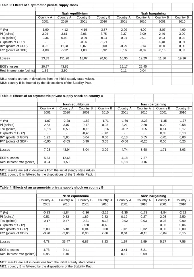
The shock provokes a steadily decrease in the output of both countries which will be equal to 4% in the long run for each (see table 2 – this one and all other tables or graphs are gathered at the end of the paper –). Inflation increases immediately from 3 and 2 percentage points for countries A and B, respectively, and stabilises 4 percentage points higher than in the pre-shock situation.
Since the ECB is supposed to have a preference for inflation stability over output stability16, the nominal interest rate is raised so that the real interest rate be increased by almost 200 basis points in the short run, and almost 300 in the long run. This policy has two types of effects in the model: first, it dampens inflationary trends in the short run through its negative effect on aggregate demand. Second, it raises net interests sharply and is likely to put heavy pressure on fiscal policy.
Government A tries to focus on the output deviations and to offset the negative shock: the tax rate is reduced in the short run. The resulting steep growth in public debt (which is also due to the feedbacks of the higher real interest rate on public net interests) leads government A to increase the tax rate in the long run. This way, it reduces the inflationary consequences of public debt accumulation. Public debt nonetheless stabilises at an unprecedenting peak: 11 points of GDP over its initial steady-state value! The reversal of fiscal policy in country A between the short and the long run is enlightening on the effects of public debt on inflation: debt is inflationary, not because there is any seigniorage or inflation surprise, but because it incorporates a wealth effect. The existence of Ricardian consumers enables government A to be also non-Ricardian: it does not have to satisfy ex ante its “intertemporal budget constraint” because it is well aware that macroeconomic mechanisms at equilibrium will bear the costs of satisfying its constraint ex post.
As for government B, it is able to reduce the tax rate in the short and in the long run, because its spending is set in accordance with the satisfaction of a constant public debt to GDP ratio. In the short run, the constraint on its public deficit puts a heavy weigth on its capacity to stabilise the output: it departs in absolute value by more than 4% from its initial steady state level, whereas the deviation of output in country A is below 2%. In the mid-run, however, the stability of the public debt ratio reduces inflationary pressures and their consequences on competitiveness: the trade balance increases and in the long run, country B’s net external position has grown by almost 6 points of the GDP. In fine, output in country B stabilises slightly closer to the initial steady state in comparison with country A.
Losses for both governments are quite similar in the short run, but at odds in the long run: the difference between both depends quite exclusively on fiscal instruments and public debts. The short term fiscal policy by government A is very costly in the longer run: as stated earlier, public debt soars and necessitates that the tax rate be increased by almost 1 point – in comparison, the tax rate in country B moves by 0.3 point in absolute value –. Note also that the more restrictive monetary policy, the costlier fiscal policy in country A.
16
In the statutes of the European Central Bank in Frankfurt, it is well specified that the primary target for the Bank is “to maintain price stability” and that output stability might be a second objective insofar as “it does not jeopardise the primary one”.
What could be learned from this equilibrium? First, in our setting, the government with sound public finances, and thus able to make its public deficit depart from the steady state, is more able to stabilise the output the closest to the initial equilibrium. Second, it is less able to curb inflation. In this strategy, it is outpaced by the government whose hands are tied. In the long run, the government with initial sound public finance incurs a reversal in its fiscal policy: public debt has increased so much that stopping its growth has become the primary objective of the fiscal policy maker. Had he followed a “time-consistent fiscal policy”, which would have prevented him from changing his fiscal policy from the short to the long run17, he would have had to choose between a low debt-low inflation-low output situation and a high debt-high inflation-high output one. Whatever its decision, its capacity to circumvent one part of the shock (on the output or on inflation) in the short run or in the long run would have been reduced. Although this would have to be more carefully verified, it is not sure that “time-consistent policies” would give better results for country A in terms of deviations of output, inflation and fiscal instrument from their respective targets.
4.1.2. The gains from coordination
Coordination between the three policy makers make each country face a more equitable share of the burden of the shock in the short run and increases the homogeneity in their business cycles in the long run. Output decreases more in country A with coordinated policies in comparison with the Nash equilibrium, whereas it decreases less in country B; inflation increases less in country A in comparison with the Nash equilibrium, whereas it increases more in country B.
This way, losses for both governments are close one to the other in the short and in the long run. Coordination is also the most productive for government A in the short run since its loss is now lower than the one incurred by government B, a situation which was the opposite after uncoordinated policies. This new result depends on fiscal and monetary policy. The latter is very slightly restrictive (the real interest rate rises by 10 basis points, in comparison with 200 when policies were uncoordinated), so that fiscal policy begins to be restrictive (rather than expansionary in the Nash equilibrium) – between 2000 and 2001, the tax rate increases by 0.3 point from its initial value –, and then neutral (rather than restrictive in the Nash equilibrium). Public debt therefore remains almost stable in proportion to the GDP.
Coordinated policies give rise to a change in the assignment of instruments – monetary and fiscal – to targets. Whereas government A had a preference for the output target while the ECB had a preference for the inflation target at the Nash equilibrium, they now seem to have switched their preferences: government A tries to offset the inflationary consequences of the shock via a reduction in consumption (the disposable income is reduced) and, thanks to government A which dampens the long run inflationary pressure due to the increase in net wealth, the ECB does not implement a monetary policy restrictive enough to curb inflation as early as in the short run.
Due to the homogeneity of the business cycles in the monetary union, trade balances and the net external positions are stable at their initial steady state values. Coordination has therefore increased the convergence of both economies in the face of a symmetric shock but, whereas a substantial part of the stabilisation process was realised
17
through the real wealth effect at the Nash equilibrium, it is no more the case when policies are coordinated.
4.2 Asymmetric supply shocks
The economic dynamics after an asymmetric shock, whether on country A or country B, is almost the same as after a symmetric shock, except for the size of the values (see tables 3 and 4).
4.2.1. The Nash equilibrium
We concentrate on some peculiar points – differences between the two asymmetric shocks or the setting of economic policies –. First, while the country which is not hit by the shock does not suffer much from inflationary pressure, this feedback is the smaller in the short run, the more constrained the government; and the smaller in the long run, the less constrained the government. In the first case, government B does not implement an expansionary fiscal policy, contrary to government A when it is not hit by the shock. In the second case, government A is able to implement a restrictive policy which helps to curb inflation. Government B does not. Of course, the capacity of government A to expand its deficit in the short run, though its unfavourable impact on inflation, has positive consequences in terms of GDP deviations from the steady state: the decrease in the output is smaller for government A than for government B when they are respectively not hit by the shock.
When comparing a shock on country A or country B, it is worth noting that monetary and fiscal policies are almost the same. Monetary policy is more restrictive in the long run than in the short run in both cases, with the real interest rate departing from the initial steady state by 1.5 point in the long run. Public debt in country A increases by 2 points of GDP in the short run and 5.5 points in the long run. The fact that the supply shock increases inflation in one country and decreases GDP growth in both countries necessitates the same kind of fiscal policy in the short run, whatever the country hit by the shock, and the same kind of monetary policy because, on average, the inflation rate and GDP deviations have grown by the same amount. The strong interactions between strategic policies highly depends on the degree of interdependence between both countries in terms of output, via the trade balance and the net external position (linked to the aggregate demand by the wealth effect).
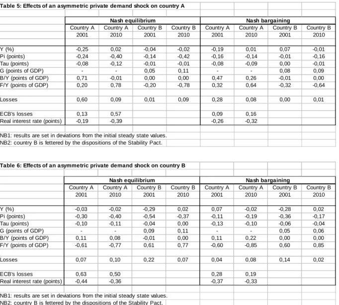
The situation after an asymmetric demand shock is totally different (see tables 5 and 6): the size of fiscal and monetary actions are not comparable if the shock hits country A or B. After a demand shock, there is no tension between inflation and output targets for the three policy makers. Monetary and fiscal authorities implement expansionary policies in the short run. If the shock occurs in country A, the capacity of its government to increase the public deficit does not necessitate a sharp decrease in the real interest rate. Government A is hence caught into a vicious circle: because it is able to react to the shock, monetary policy is not as expansionary as in the case of a symmetric shock, nor as in the case of a shock on B (see table 6), but the low decrease in the interest rate in turn reduces the fiscal room for maneuver. The resulting public debt to GDP increases sharply in the short run. If the shock occurs in country B, the central bank must bear a higher burden of the shock since government B is unable to react to the shock: the real interest rate decreases more than in the case of a shock on country A. The limitations on fiscal policy in country B have feedback effects on country A whose tax
rate is reduced by more than after a shock on country A. Public debt keeps closer to the initial steady state, however, because net interests have been lessened by the expansionary monetary policy. Fiscal policy by government A is thus implemented more easily than in the preceding case.
4.2.2. The Nash bargaining solutions
First, the fact that one country is able to react to the asymmetric supply shock by a non-neutral fiscal policy makes coordination less productive. Gains form coordination are very small, as regards the symmetric shock. One reason for this is that the ability of government A to implement an active (in the sense of Leeper) policy does not necessitate a tough coordination with government B and the ECB.
Second, the resulting tension between inflation and output targets after an asymmetric supply shock is more accurate than after a symmetric shock, when coordinated policies are implemented. Monetary policy concentrates more on the inflation target and the real interest rate is raised by 20 basis points, hence twice its rise after a symmetric shock (with Nash bargaining solutions). The resulting increase in the public debt to GDP ratio in country A is higher after a shock on this country than on country B or after a symmetric shock.
Third, we do not find any clear-cut reversal in the assignment of instruments to targets when policies are coordinated, contrary to the situation following a symmetric shock.
The difficulties to coordinate monetary and fiscal policies after a shock on country A are such that the losses for government A at the coordinated equilibrium are higher when it is hit by the shock than government B’s when country B is hit by the shock. The losses of the ECB are also higher in the case of a shock on country A than on country B.
It is worth noting that after an asymmetric demand shock on country B, gains from coordination are substantial for the ECB. This is consistent with the fact that the compliance of government B to a balanced-budget rule has ‘beggar-thy-neighbour’ effects (more activism by the ECB) which cooperation can contribute to reduce. Gains for government A are nonetheless very small, most notably because the lower activism by the ECB provokes a higher activism by government A: its public debt to GDP ratio, for instance, departs more from the steady state with coordinated policies than without (table 6).
5. The costs of the Stability Pact
Now that the economic dynamics behind supply as well as demand shocks has been explained, we turn to a more fundamental question: does the asymmetry in the fiscal setting between the two countries forming a monetary union has negative feedback consequences on the government with initial sound public finances and the ECB? Do these feedback effects depend on the nature of the shock (supply or demand, symmetric or asymmetric)? To answer these questions, we study the losses the policy makers have incurred after the various exogenous shocks.
5.1. The situation of the governments
At the Nash equilibrium, in the case of a symmetric or of an asymmetric shock on country B, whether a supply or a demand one, the fact that one government is constrained by the dispositions of the Stability and Growth Pact may force the other, more solvent, government to bear the brunt of shocks – it is this government, and not the constrained one, that bears the major part of these shocks. This appears clearly in graphs 1 and 2. As early as 4 or 7 quarters after the supply shocks, symmetric and asymmetric respectively, government A faces a higher loss than government B, due notably to the substantial increase in the public debt to GDP ratio.
It is interesting to compare also the losses incurred by government A when country A is not hit by the shock with the losses incurred by government B when country B is not hit by the shock. Results are reported in graphs 3 (supply shocks) and 4 (demand shocks). In the case of supply shocks, losses for both governments are the same in the first year after the shocks; then the discrepancy is very high and shows how much country A is fettered indirectly by the dispositions of the Stability Pact. With demand shocks, government A is always in a worse situation than government B, when both are not hit by the shock.
The country with sound public finances undergoes two types of feedback effects. First, as already mentioned, it has to participate in the stabilisation of the whole monetary union, even if it is not directly hit by the shock. The interdependence between the economies increases the strategic interactions between fiscal policies. Second, these interactions also involve monetary policy. In this peculiar setting, which hinges on an extended version of the macroeconomic model of the Fiscal Theory of the Price Level developed by LWL (2000), the government of country A has to stop the public debt to GDP ratio from increasing because monetary policy is active (the nominal interest rate reacts more than one for one with the inflation rate). Government A is therefore fettered in its policy choices by the growth in its debt and by the relative stringency of monetary policy.
Nash bargaining solutions in the case of supply shocks are highly productive in that they cancel the costs emerging from the Stability Pact. As shown in graph 5, losses for governments A and B when they are not hit by the shock respectively are now almost equal, the differences between them being only marginal. If the shock falls on country B, government B now bears the major burden of the shock: its loss is clearly superior to the ECB’s and government A’s (graph 6). After a symmetric supply shock (graph 7), losses for both governments are exactly similar: the share of the burden has therefore been greatly improved by the coordination of fiscal and monetary policies.
This improvement does not emerge after a demand shock (see graph 8). Government A remains in a worse situation than government B when they are not hit by the shock respectively, although economic policies are coordinated and improve the situation of the three authorities in comparison with the Nash equilibrium. As already mentioned, this is mainly due to the variations in the real interest rates (see graphs 9 and 10): if the demand shock occurs in country B, monetary policy is less active with coordinated policies than without – this is unfavourable to government A –; but if the shock occurs in country A, the reverse is true until the mid-run – this is favourable to both governments –.
5.2. What about the ECB?
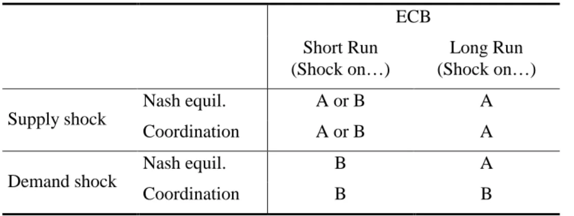
In table 7 below, we have reported the worst situations for the ECB after an asymmetric shock has occurred in one country of the monetary union. In the short run, both asymmetric supply shocks induce the same amount of welfare losses for the central bank In the long run however, a supply shock is always the most costly for the ECB if it has occurred in country A. This result is explained by the higher inflationary impact of the shock and by the higher deviation of the real interest rate from the initial steady state when the shock hits country A rather than country B (see graph 11).
Table 7: The most costly asymmetric shock for the ECB (based on loss values)
ECB Short Run (Shock on…) Long Run (Shock on…) Nash equil. A or B A Supply shock Coordination A or B A Nash equil. B A Demand shock Coordination B B
After a demand shock, the ECB incurs a larger welfare loss in the short run if the shock occurs in country B rather than A. This is consistent with the more substantial participation of the central bank in the management of the shock when the fiscally-contrained country is hit by the shock. As shown in graph 12, the decrease in the real interest rate is more pronounced in this case than after a shock on country A. In the long run, however, this more intense monetary policy seems productive: the ECB’s loss is lower than after a shock on country A (see graph 13) and the real interest rate now departs less from its steady state than in any other situation with a demand shock. This situation is reversed if policies are coordinated. Indeed, until the long run, monetary policy is more involved in the shock on B than on A (the real interest rate falls more in the first case than in the second one, see graph 14), so that the better welfare situation for the ECB is the occurrence of a demand shock in country A (see graph 15).
The costs induced by the Stability and Growth Pact for the ECB are twofold. First, the Pact implies more interventions by the ECB in order to offset the demand shock if it has occurred in the fiscally-constrained country (country B) rather than in the country with sound public finance (country A). Second, if the occurrence of a supply shock in country A is more costly for the ECB than a supply shock on country B, one does have to keep in mind that, had country B not been fiscally-constrained, it would have implemented the kind of fiscal policy country A implemented although it had not been hit by the shock: this latter policy was able to increase the welfare of the country directly hit by the shock as well as the ECB’s. In this case, the costs due to the Stability Pact are indirect.
5. Conclusion
In this paper, we have used an extended version of Leith & Wren-Lewis (2000) model to the open-economy with asymmetric frameworks for the governments. We have illustrated some possible drawbacks of the Stability and Growth Pact, namely the fact that it may reduce the ability of governments and the ECB to implement stabilisation policies in the Euro area. The model by LWL enables a precise and comprehensive analysis of the interactions between monetary and fiscal policies. The most recent contributions concerning monetary rules, fiscal rules, and the net wealth effect are included and shed light on the effects of public debt on the inflation rate, without having to introduce such old-fashioned thing as seignoriage and the like.
Within this dynamic and patrimonial framework, we have been able to distinguish clearly between the short-run and long-run effects of economic policies. For instance, we showed that debt implications are substantial: they change the timing of fiscal policy. From ‘active’ in the short run, they become ‘passive’ in the long run, undergoing the law of an active monetary policy.
Main results are the following. First, after a symmetric supply shock, the coordination of policies give rise to a change in the assignment of instruments – monetary and fiscal – to targets. The government with initial sound public finances now dampens the inflationary consequences of the shock and the monetary policy is substantially less restrictive than at the uncoordinated equilibrium. This switch in the assignment of instruments does not occur after a symmetric demand shock or any asymmetric shock.
Second, the country with sound public finances undergoes two types of feedback effects. It has to intervene in order to stabilise the whole monetary union, even if it is not directly hit by the shock. The interdependence between the economies thus increases the strategic interactions between fiscal policies. But it also increases the interactions between fiscal and monetary policies: because of the growth of public debt and the relative stringency of monetary policy, the government of this country is more and more fettered in its policy choices as time moves forward.
Third, coordination in the case of asymmetric supply shocks is very productive because it cancels the costs emerging from the Stability Pact. The major share of the burden of the shock now falls on the country directly hit by the shock, be it fiscally or not-fiscally constrained. This result does not emerge after a demand shock.
Last, the costs induced by the Stability and Growth Pact for the ECB are twofold. On the one hand, the Pact implies more interventions by the ECB in order to offset the demand shock if it has occurred in the fiscally-constrained country rather than in the country with sound public finance. On the other hand, after a supply shock, the costs due to the Stability Pact are mostly indirect.
Results therefore showed that a stringent application of the provisions of the Stability and Growth Pact may substantially fetter economic policies in the whole Euro area. Most noteworthy, the Pact impinges negatively on fiscally ‘virtuous’ policy makers: countries with sound public finances can incur a substantial public debt burden after a shock has hit a country with ‘unsound’ public finances. In this sense, the Pact seems ill-designed.
The sub-optimality of the Stability Pact for Euro-area countries will also have effects on the rest of the world, at least through the Euro exchange rate. The fact that the European nominal interest might be set at an excessive level due to cooperation failures between intra-European authorities might influence the level as well as the volatility of the Euro-US Dollar exchange rate. Our future research should now be aimed at adding a “rest of the world” in the model in order to analyse the interactions between European monetary and fiscal policies and the determination of the Euro exchange rate.
6. References
ALESINA A. & R. PEROTTI (1995), “Fiscal Expansions and Adjustments in OECD Countries”, Economic Policy, 21.
BARRO R.J. (1974), “Are Government Bonds Net Wealth ?”, Journal of Political
Economy, 82, November-December.
BARRO R.J. (1979), “On the Determination of the Public Debt”, Journal of Political Economy, 87(5).
BARRELL R. & J. SEFTON (1997), “Fiscal Policy and the Maastricht Solvency
Criteria”, The Manchester School, 65(3), June.
BEETSMA R.M.W.J. & H. UHLIG (1999), “An Analysis of the Stability and Growth Pact”, Economic Journal, 109(458), October.
BERGIN P.R. (2000), “Fiscal Solvency and Price Level Determination in a Monetary
Union”, Journal of Monetary Economics, 45(1), February.
BLAKE A. et M. WEALE (1998), “Costs of Separating Budgetary Policy From Control of Inflation: a Neglected Aspect of Central Bank Independence”, Oxford Economic Papers, 50, July.
BLANCHARD O.J. (1985), “Debt, Deficits, and Finite Horizons”, Journal of Political
Economy, 93(2), April.
BUITER W.H. (2000), “The Fallacy of the Fiscal Theory of the Price Level , again”,
mimeo, May.
BUITER W.H. (1989), “The Superiority of Contingent Rules over Fixed Rules in
Models with Rational Expectations”, in BUITER W.H. (ed.), Macroeconomic Theory and Stabilisation Policy, Manchester University Press.
CAPOEN F. & P. VILLA (1997), “Internal and External Policy Coordination: a
Dynamic Analysis”, CEPII Working Paper n°97-15, November.
CHARI V.V. & P.J. KEHOE (1998), “On the Need for Fiscal Constraints in a Monetary Union”, Federal Reserve Bank of Minneapolis Working Paper n°589, August. CHARI V.V., P.J. KEHOE & E.C. PRESCOTT (1989), “Time Consistency and Policy”,
in BARRO R.J. (ed.), Modern Business Cycles Theory, Basil Blackwell.
FUHRER J.C. (1997), “The (Un)Importance of Forward-Looking Behavior in Price Specifications”, Journal of Money, Credit, and Banking, 29(3), August.
HUGHES HALLETT A.J. (1986), “Autonomy and the Choice of Policy in
HUGHES HALLETT A.J. & D. VINES (1993), “On the Possible Costs of European
Monetary Union”, The Manchester School, 61(1), March.
JENSEN S.E.H. (1997), “Wage Rigidity, Monetary Integration and Fiscal
Stabilization in Europe”, Review of International Economics, Special Supplement, 5(4). JENSEN S.E.H. & L.G. JENSEN (1995), “Debt, Deficits and Transition to EMU: a
Small Country Analysis”, European Journal of Political Economy, 11(1), March.
LE BIHAN H. & F. LERAIS (1998), “Simulations Properties of MIMOSA, a
macroeconometric multinational model”, MIMOSA Working Paper,OFCE, n°M-98-01, January.
LEEPER E. (1991), “Equilibria under ‘Active’ and ‘Passive’ Monetary Policies”,
Journal of Monetary Economics, 27.
LEITH C. & S. WREN-LEWIS (2000), “Interactions between Monetary and Fiscal Policies”, Economic Journal, 110, March.
PLOEG F. (van der) (1995), “Solvency of Counter-Cyclical Policy Rules”, Journal
of Public Economics, 57.
SACHS J. & C. WYPLOSZ (1984), “La Politique Budgétaire et le Taux de Change Réel”, Annales de l’INSEE, 53, January-March.
TOBIN J. & W.H. BUITER (1976), “Long-run Effects of Fiscal and Monetary Policy
on Aggregate Demand”, in STEIN J.L. (ed.), Monetarism, North Holland.
WOODFORD M. (1996), “Control of the Public Debt: a Requirement for Price
Stability?”, NBER. Working Paper n°5684, July (published in a shorter version in G. CALVO & M. KING, eds., The Debt Burden and its Consequences for Price Stability, St
Martin’s Press, 1998).
7. Tables and graphs
Table 2: Effects of a symmetric private supply shockCountry A Country A Country B Country B Country A Country A Country B Country B 2001 2010 2001 2010 2001 2010 2001 2010 Y (%) -1,90 -4,12 -4,19 -3,87 -2,99 -4,00 -3,07 -4,00 Pi (points) 3,04 3,61 2,06 3,75 2,37 3,09 2,40 3,09 Tau (points) -0,36 0,98 -0,39 -0,34 -0,01 0,01 0,03 0,02 G (points of GDP) - - -0,96 -1,21 - - -0,01 0,01 B/Y (points of GDP) 3,92 11,34 0,07 0,00 -0,29 0,14 0,00 0,00 F/Y (points of GDP) -1,80 -5,92 1,80 5,92 0,16 -0,07 -0,16 0,07 Losses 23,33 151,28 18,07 20,66 10,95 19,20 11,36 19,16 ECB's losses 20,77 43,85 15,17 25,45
Real interest rate (points) 1,89 2,90 0,11 0,04 NB1: results are set in deviations from the initial steady state values.
NB2: country B is fettered by the dispositions of the Stability Pact.
Nash equilibrium Nash bargaining
Table 3: Effects of an asymmetric private supply shock on country A
Country A Country A Country B Country B Country A Country A Country B Country B
2001 2010 2001 2010 2001 2010 2001 2010 Y (%) -1,07 -2,28 -1,82 -1,71 -1,59 -2,23 -1,35 -1,77 Pi (points) 2,53 3,07 0,17 0,93 2,21 2,80 0,29 0,58 Tau (points) -0,18 0,50 -0,18 -0,16 -0,02 0,05 0,14 0,17 G (points of GDP) - - -0,46 -0,61 - - 0,09 0,13 B/Y (points of GDP) 1,92 5,85 0,04 0,00 0,13 0,55 -0,01 0,00 F/Y (points of GDP) -0,90 -3,05 0,90 3,05 -0,06 -0,25 0,06 0,25 Losses 7,93 43,94 3,04 3,09 4,74 8,68 1,71 3,03 ECB's losses 5,63 12,65 4,18 7,57
Real interest rate (points) 0,94 1,50 0,18 0,16
NB1: results are set in deviations from the initial steady state values. NB2: country B is fettered by the dispositions of the Stability Pact.
Nash equilibrium Nash bargaining
Table 4: Effects of an asymmetric private supply shock on country B
Country A Country A Country B Country B Country A Country A Country B Country B
2001 2010 2001 2010 2001 2010 2001 2010 Y (%) -0,83 -1,84 -2,36 -2,16 -1,35 -1,78 -1,84 -2,22 Pi (points) 0,51 0,53 1,89 2,83 0,19 0,27 2,05 2,50 Tau (points) -0,17 0,47 -0,21 -0,18 -0,02 0,03 0,08 0,09 G (points of GDP) - - -0,50 -0,60 - - 0,05 0,06 B/Y (points of GDP) 2,00 5,48 0,04 0,00 -0,01 0,32 0,00 0,00 F/Y (points of GDP) -0,90 -2,86 0,90 2,86 0,04 -0,15 -0,04 0,15 Losses 4,78 33,47 6,87 8,23 1,67 2,99 5,17 7,56 ECB's losses 4,78 9,41 3,41 5,21
Real interest rate (points) 0,95 1,40 0,12 0,09
NB1: results are set in deviations from the initial steady state values. NB2: country B is fettered by the dispositions of the Stability Pact.
Table 5: Effects of an asymmetric private demand shock on country A
Country A Country A Country B Country B Country A Country A Country B Country B
2001 2010 2001 2010 2001 2010 2001 2010 Y (%) -0,25 0,02 -0,04 -0,02 -0,19 0,01 0,07 -0,01 Pi (points) -0,24 -0,40 -0,14 -0,42 -0,16 -0,14 -0,01 -0,16 Tau (points) -0,08 -0,12 -0,01 -0,01 -0,08 -0,09 0,00 -0,01 G (points of GDP) - - 0,05 0,11 - - 0,08 0,09 B/Y (points of GDP) 0,71 -0,01 0,00 0,00 0,47 0,26 -0,01 0,00 F/Y (points of GDP) 0,20 0,78 -0,20 -0,78 0,32 0,64 -0,32 -0,64 Losses 0,60 0,09 0,01 0,09 0,28 0,08 0,00 0,01 ECB's losses 0,13 0,57 0,09 0,16
Real interest rate (points) -0,19 -0,39 -0,26 -0,32
NB1: results are set in deviations from the initial steady state values. NB2: country B is fettered by the dispositions of the Stability Pact.
Nash equilibrium Nash bargaining
Table 6: Effects of an asymmetric private demand shock on country B
Country A Country A Country B Country B Country A Country A Country B Country B
2001 2010 2001 2010 2001 2010 2001 2010 Y (%) -0,03 -0,02 -0,29 0,02 0,07 -0,02 -0,28 0,02 Pi (points) -0,30 -0,40 -0,54 -0,37 -0,11 -0,19 -0,36 -0,17 Tau (points) -0,10 -0,11 -0,04 0,00 -0,13 -0,10 -0,06 -0,04 G (points of GDP) - - 0,09 0,11 - - 0,05 0,06 B/Y (points of GDP) 0,11 0,08 -0,01 0,00 0,11 0,22 0,00 0,00 F/Y (points of GDP) -0,61 -0,77 0,61 0,77 -0,60 -0,85 0,60 0,85 Losses 0,07 0,10 0,22 0,07 0,04 0,08 0,14 0,02 ECB's losses 0,63 0,50 0,28 0,19
Real interest rate (points) -0,44 -0,36 -0,37 -0,33
NB1: results are set in deviations from the initial steady state values. NB2: country B is fettered by the dispositions of the Stability Pact.
Graph 1: Losses - Symmetric supply shocks - Nash equilibrium 0 20 40 60 80 100 120 140 160 2000 2001 2002 2003 2004 2005 2006 2007 2008 2009 2010 2011 2012 2013 2014 2015 2016 2017 2018 2019 Gvt A Gvt B ECB
Graph 2: Losses - Supply shock on B - Nash equilibrium
0 5 10 15 20 25 30 35 40 2000 2001 2002 2003 2004 2005 2006 2007 2008 2009 2010 2011 2012 2013 2014 2015 2016 2017 2018 2019 Gvt A Gvt B ECB
Graph 3: Losses for Gvts A and B when they are not hit by the asymmetric supply shock Nash equilibrium 0 5 10 15 20 25 30 35 40 2000 2001 2002 2003 2004 2005 2006 2007 2008 2009 2010 2011 2012 2013 2014 2015 2016 2017 2018 2019 Gvt A - shock on B Gvt B - shock on A
Graph 4: Losses for Gvts A and B when they are not hit by the asymmetric demand shock Nash equilibrium 0 0,02 0,04 0,06 0,08 0,1 0,12 2000 2001 2002 2003 2004 2005 2006 2007 2008 2009 2010 2011 2012 2013 2014 2015 2016 2017 2018 2019 Gvt A - shock on B Gvt B - shock on A
Graph 5: Losses for Gvts A and B when they are not hit by the asymmetric supply shock Nash bargaining 0 0,5 1 1,5 2 2,5 3 3,5 2000 2001 2002 2003 2004 2005 2006 2007 2008 2009 2010 2011 2012 2013 2014 2015 2016 2017 2018 2019 Gvt A - shock on B Gvt B - shock on A
Graph 6: Losses - Supply shock on B - Nash bargaining
0 1 2 3 4 5 6 7 8 2000 2001 2002 2003 2004 2005 2006 2007 2008 2009 2010 2011 2012 2013 2014 2015 2016 2017 2018 2019 Gvt A Gvt B ECB
Graph 7: Losses - Symmetric supply shock - Nash bargaining 0 5 10 15 20 25 30 2000 2001 2002 2003 2004 2005 2006 2007 2008 2009 2010 2011 2012 2013 2014 2015 2016 2017 2018 2019 Gvt A Gvt B ECB
Graph 8: Losses for Gvts A and B when they are not hit by the asymmetric demand shock Nash bargaining 0 0,01 0,02 0,03 0,04 0,05 0,06 0,07 0,08 0,09 2000 2001 2002 2003 2004 2005 2006 2007 2008 2009 2010 2011 2012 2013 2014 2015 2016 2017 2018 2019 Gvt A - shock on B Gvt B - shock on A
Graph 9: Demand shock on country B - Real interest rate -0,5 -0,45 -0,4 -0,35 -0,3 -0,25 -0,2 -0,15 -0,1 -0,05 0 2001 2002 2003 2004 2005 2006 2007 2008 2009 2010 2011 2012 2013 2014 2015 2016 2017 2018 2019 Nash equilibrium Nash bargaining
Graph 10: Demand shock on country A - Real interest rate
-0,45 -0,4 -0,35 -0,3 -0,25 -0,2 -0,15 -0,1 -0,05 0 2001 2002 2003 2004 2005 2006 2007 2008 2009 2010 2011 2012 2013 2014 2015 2016 2017 2018 2019 Nash equilibrium Nash bargaining
Graph 11: Supply shocks - Real interest rates - Nash equilibrium 0 0,5 1 1,5 2 2,5 3 3,5 2000 2001 2002 2003 2004 2005 2006 2007 2008 2009 2010 2011 2012 2013 2014 2015 2016 2017 2018 2019 Symm. Shock Shock on A Shock on B
Graph 12: Demand shocks - Real interest rates - Nash equilibrium
-0,8 -0,7 -0,6 -0,5 -0,4 -0,3 -0,2 -0,1 0 2000 2001 2002 2003 2004 2005 2006 2007 2008 2009 2010 2011 2012 2013 2014 2015 2016 2017 2018 2019 Symm. Shock Shock on A Shock on B
Graph 13: Demand shocks - Monetary losses - Nash equilibrium 0 0,5 1 1,5 2 2,5 2000 2001 2002 2003 2004 2005 2006 2007 2008 2009 2010 2011 2012 2013 2014 2015 2016 2017 2018 2019 Symm. Shock Shock on A Shock on B
Graph 14: Demand shocks - Real interest rates - Nash bargaining
-0,8 -0,7 -0,6 -0,5 -0,4 -0,3 -0,2 -0,1 0 2000 2001 2002 2003 2004 2005 2006 2007 2008 2009 2010 2011 2012 2013 2014 2015 2016 2017 2018 2019 Symm. Shock Shock on A Shock on B
Graph 15: Demand shocks - Monetary losses - Nash bargaining 0 0,1 0,2 0,3 0,4 0,5 0,6 0,7 0,8 0,9 1 2000 2001 2002 2003 2004 2005 2006 2007 2008 2009 2010 2011 2012 2013 2014 2015 2016 2017 2018 2019 Symm. Shock Shock on A Shock on B