Manipulator motion planning for high-speed robotic laser cutting

HAL Id: hal-00513036

https://hal.archives-ouvertes.fr/hal-00513036

Submitted on 1 Sep 2010

HAL is a multi-disciplinary open access archive for the deposit and dissemination of sci-entific research documents, whether they are pub-lished or not. The documents may come from teaching and research institutions in France or abroad, or from public or private research centers.

L’archive ouverte pluridisciplinaire HAL, est destinée au dépôt et à la diffusion de documents scientifiques de niveau recherche, publiés ou non, émanant des établissements d’enseignement et de recherche français ou étrangers, des laboratoires publics ou privés.

Alexandre Dolgui, Anatol Pashkevich

To cite this version:

Alexandre Dolgui, Anatol Pashkevich. Manipulator motion planning for high-speed robotic laser cutting. International Journal of Production Research, Taylor & Francis, 2009, 47 (20), pp.5691-5715. �10.1080/00207540802070967�. �hal-00513036�

For Peer Review Only

Manipulator motion planning for high-speed robotic laser cutting

Journal: International Journal of Production Research Manuscript ID: TPRS-2008-IJPR-0234

Manuscript Type: Original Manuscript Date Submitted by the

Author: 18-Mar-2008

Complete List of Authors: Dolgui, Alexandre; Ecole des Mines de St Etienne, Division for Indl Engineering and Computer Sciences

Pashkevich, Anatol; Belarusian State University of Informatics and Radioelectronics, Robotic Laboratory

Keywords: PATH PLANNING, OPTIMIZATION, SIMULATION Keywords (user): PATH PLANNING, OPTIMIZATION

For Peer Review Only

Manipulator motion planning for high-speed robotic laser cutting

ALEXANDRE DOLGUI

1

and ANATOL PASHKEVICH

1,2

1

Centre for Industrial Engineering and Computer Science Ecole de Mines de Saint Etienne,

158, Cours Fauriel, 42023 Saint Etienne, France e-mail: dolgui@emse.fr

2

Department of Automatics and Production Systems Ecole des Mines de Nantes,

4 rue Alfred-Kastler, Nantes 44307,France e-mail: anatol.pashkevich@emn.fr

Keywords: Robot path planning; Laser beam cutting; Multiple-criteria optimisation Corresponding author:

Prof. Alexandre Dolgui,

Centre for Industrial Engineering and Computer Science

Ecole de Mines de Saint Etienne, 158, cours Fauriel, 42023 Saint Etienne, France Tel. : +33 (0)4.77.42.01.66, Fax : +33 (0)4.77.42.66.66 E-mail : dolgui@emse.fr 1 2 3 4 5 6 7 8 9 10 11 12 13 14 15 16 17 18 19 20 21 22 23 24 25 26 27 28 29 30 31 32 33 34 35 36 37 38 39 40 41 42 43 44 45 46 47 48 49 50 51 52 53 54 55 56 57 58 59 60

For Peer Review Only

Manipulator motion planning

for high-speed robotic laser cutting

Alexandre DOLGUI1 and Anatol PASHKEVICH1,2

1

Division for Industrial Engineering and Computer Sciences

Ecole de Mines de Saint Etienne, 158, Cours Fauriel, 42023 Saint Etienne, France e-mail: dolgui@emse.fr

2

Department of Automatics and Production Systems

Ecole des Mines de Nantes

4 rue Alfred-Kastler, Nantes 44307,France, e-mail: anatol.pashkevich@emn.fr

Abstract: Recent advances in laser technology, and especially the essential increase of the

cutting speed, motivate amending the existing robot path methods, which do not allow the complete utilisation of the actuator capabilities as well as neglect some particularities in the mechanical design of the wrist of the manipulator arm. This research addresses the optimisation of the 6-axes robot motions for continuous contour tracking while considering the redundancy caused by the tool axial symmetry. The particular contribution of the paper is in the area of multi-objective path planning using graph-based search space representation. In contrast to previous works, the developed optimisation technique is based on the dynamic programming and explicitly incorporates the verification of the velocity/acceleration constrains. This allows the designer to define interactively their importance with respect to the path-smoothness objectives. In addition, this optimisation technique takes into account the capacity of some manipulator wrist axes for unlimited rotation in order to produce more economical motions. The efficiency of the developed algorithms has been carefully investigated via computer simulation. The presented results are implemented in a commercial software package and verified for real-life applications in the automotive industry.

Keywords: Robot path planning; Laser beam cutting; Multiple-criteria optimisation.

1 2 3 4 5 6 7 8 9 10 11 12 13 14 15 16 17 18 19 20 21 22 23 24 25 26 27 28 29 30 31 32 33 34 35 36 37 38 39 40 41 42 43 44 45 46 47 48 49 50 51 52 53 54 55 56 57 58 59 60

For Peer Review Only

1. Introduction

Laser cutting processes have become increasingly important in a wide range of industrial applications due to their many advantages over other cutting methods. The key features of this technology include high speed, narrow kerf width, small thermal distortions and very low roughness on the edges that allow non-contact processing of complex 3D shapes without additional finishing operations. To ensure high productivity and flexibility, the laser is usually manipulated by either a CNC machine or a 5/6-axis industrial robot, which is programmed off-line using available commercial CAD/CAM systems (Nof, 1999; Gropp et al., 1995; Defaux, 2004; Ion, 2005). However, recent advances in the laser cutting technologies motivate enhancements of existing programming methods and encourage developments of dedicated optimisation algorithms that are in the focus of this paper.

The most important aspect of this problem is related to essential increase of the technologically admissible limit for the cutting speed. At present, depending on the laser configuration, and also on a type and thickness of the processing material, the cutting speed can reach more than 50 m/min. This is comparable with the kinematic capabilities of modern industrial robots, which are used to manipulate the laser beam (Steen, 2003; Rooks, 2004; Schlueter, 2005). For instance, for a typical 6-axis anthropomorphic robot, the forearm axis speeds range from 200 to 300 deg/sec and the wrist axes may be actuated with speed from 300 to 500 deg/sec. However, the maximum Cartesian velocity of the tool is usually lower than 1 m/s and significantly varies over the workspace, imposing critical constrains for the implementation of the high-speed laser cutting process. Hence, in this area, the problem of optimal motion planning for a multi-axe manipulator becomes crucial. However, as follows from our experience, direct application of existing algorithms may produce unfeasible results with non-smooth velocity/acceleration profiles (in spite of a quite satisfactory performance for the lower desired cutting speed). For example, as reported in (Ghany et al., 2006), some existing path planning methods may produce cutting head vibrations at high speeds.

1 2 3 4 5 6 7 8 9 10 11 12 13 14 15 16 17 18 19 20 21 22 23 24 25 26 27 28 29 30 31 32 33 34 35 36 37 38 39 40 41 42 43 44 45 46 47 48 49 50 51 52 53 54 55 56 57 58 59 60

For Peer Review Only

Another motivating factor is caused by significant changes in the mechanical design of the robotic manipulators, which are not taken into account by the existing path optimisation techniques. In particular, one of the recent developments in the field of laser cutting, the Robocut system from Robotic Production Technology (www.rpt.net), employs an anthropomorphic manipulator with a standard architecture for the forearm and an innovative design of the wrist with infinite rotation of the 4th and 5th joints. This special design (without external cables to the robotic wrist) offers essential advantages, since the cycle time losses for the reverse rotations of axes after cutting can be avoided. This solution increases speeds for the wrist axes (up to 900 deg/sec), which allows achieving the Cartesian speed of 2.2m/s and acceleration of 1.4G. However, this is out of the scope of the known motion planning methods.

One of specific features of this problem is caused by a kinematic redundancy. It is clear that, from kinematical point of view, laser beam manipulation requires only five degrees of freedom. Accordingly, former robotic cutting systems employed 5-axis manipulators that possess simpler wrist mechanics but rather require sophisticated algorithms for the on-line solution of the inverse kinematics (Pashkevich, 1997). Most of the modern cutting robotic systems are based on the 6-axis robots. Obviously, this additional axe simplifies robot control and programming, while posing another problem: optimal utilisation of the additional motion capabilities.

This paper focuses on the enhancement of the path planning algorithms for the laser cutting robots by imposing additional constraints on the smoothness of the trajectory and taking into account both the manipulator kinematic redundancy and the ability of some axes for unlimited rotations. The remainder of the paper is organised as follows. Section 2 presents analysis of the previous works. Section 3 is devoted to the problem statement and describes the task model, problem constraints, design variables and objectives. Section 4 includes the main theoretical results and contributions, presenting a search space graph model, path optimisation algorithm, and techniques for the generation of the robot control code. Section 5 contains simulation results and

1 2 3 4 5 6 7 8 9 10 11 12 13 14 15 16 17 18 19 20 21 22 23 24 25 26 27 28 29 30 31 32 33 34 35 36 37 38 39 40 41 42 43 44 45 46 47 48 49 50 51 52 53 54 55 56 57 58 59 60

For Peer Review Only

their analysis. In Section 6, an industrial implementation is reported. Finally, Section 7 summarizes the main contributions and suggests some prospective research directions.

2. Related works

Since the debut of robotic laser cutting, most of the related research focused on robot off-line programming (Backes et al., 1995; Kaierle, 1999). The main reason is that, for this technology, the conventional “manual teaching” method proved to be very tedious and time-consuming, requiring a temporary exclusion of the robot from the manufacturing process and performing the operator-controlled movement of the tool along the cutting path, which has to be properly marked beforehand. In contrast, off-line programming can generate the control code by means of computer graphics, away from the factory floor. Thus, the down time may be significantly reduced, enabling very small batch sizes to become economically feasible (Sendler, 1994; Wittenberg, 1995; Mitsi et al., 2005).

At the moment, there are a number of commercial robotic off-line programming/simulation systems on the market. Some of the more commonly used are em-Workplace (RobCAD) from Tecnomatix Technologies (www.tecnomatix.com), IGRIP from Delmia (http://www.delmia.com), CimStation from Silma (www.silma.com), and Workspace (www.workspace5.com). They offer 3D graphical simulation environments with visual programming capabilities and a wide range of convenient design tools, such as robot selection, robot placement, motion simulation, cycle time calculation, and collision-free path planning. Some of these systems include process-specific modules for laser cutting. In particular, the “Robcad/Cut&Seal” module enables the semiautomatic creation of cutting contours and their conversion into linear, circular and spline motions. A similar software tool is also available from Alma (www.alma.fr) -- “act/cut3D”, which possesses some additional convenient features, including defining the head orientation for bevelled cutting, imposing "technological" tolerances, and interactive modification of the tool orientation for each point of the programme.

1 2 3 4 5 6 7 8 9 10 11 12 13 14 15 16 17 18 19 20 21 22 23 24 25 26 27 28 29 30 31 32 33 34 35 36 37 38 39 40 41 42 43 44 45 46 47 48 49 50 51 52 53 54 55 56 57 58 59 60

For Peer Review Only

However there still exists a considerable gap between the capabilities of the commercial robotic CAD systems and the requirements of a particular application. Up to now, the robot programs for many 3D cutting applications (especially for high-speed cutting) are constructed interactively and then are verified using simulation/visualization tools incorporated in the corresponding CAD system. The ultimate goal is the generation of reliable programs automatically from designs and drawings, similar to CNC-machine programming methods (Sun and Tsai, 1994, Bohez et al., 2000; Xu et al., 2002, Kim et al., 2003; Anotaipaiboon and Makhanov, 2005; Wang and Xie, 2005, Bi and Lang, 2007).

One of the first contributions in the off-line programming for the laser cutting robots was done by M. Geiger and his co-workers (University of Erlangen-Nuremberg, Germany). They developed technology-oriented approaches, which simultaneously consider the part geometry, process parameters and some properties of the machine tool (Geiger and Gropp, 1992; Geiger and Kolléra, 1994; Bauer, 1996). However, their techniques may be applied to the non-redundant kinematic structures only and based on the five-axis robots.

For manipulators with six degrees of freedom (which are redundant with respect to 3D cutting requirements), the motion planning problem was firstly addressed by Abe, Shibata and Tanie (Abe et al., 1994; Shibata et al., 1997). These authors proposed a genetic algorithm (GA) that optimises the cutting tool orientation using the evaluation function extracted from the experience of skilled operators. Informally, the operator preferences were defined as follows: “Motion of three basic (1st to 3rd) links with low response should be least so as to minimize movement of centre axis of the end-effector.” Formally, the local optimisation criteria was defined as the weighted squared sum of all axis velocities (from 1st to 6th) together with the velocity of the reference point for the 5th axis. Furthermore, for the overall optimisation with a global criterion, all local criteria were summed over the path. As follows from the presented results, the authors succeeded in the generation of manipulator motions for a relatively slow cutting speed (2m/min). However, there are a number of open questions with the application of this technique to current real-life problems (choosing of

1 2 3 4 5 6 7 8 9 10 11 12 13 14 15 16 17 18 19 20 21 22 23 24 25 26 27 28 29 30 31 32 33 34 35 36 37 38 39 40 41 42 43 44 45 46 47 48 49 50 51 52 53 54 55 56 57 58 59 60

For Peer Review Only

weighting factors, taking into account manipulator velocity/acceleration constraints and joint limits, as well as the convergence of algorithms for high-dimensional input data exported from CAD, etc.). Some recent techniques that employ the general end-effector constraints concept (Yao and Gupta, 2007) also suffer from this drawback.

The above mentioned approach has been enhanced in our previous paper (Pashkevich et al., 2004), which presents a detailed study of multiple optimisation objectives and their incorporation in the global criterion. Compared to other works, our motion planning algorithm possesses essential advantages, since it is based on a graph representation of the search space and on the dynamic programming. The latter ensures a much higher computation speed than the GA, which is very important for industrial applications. This algorithm was successfully implemented on a factory floor and later verified in the automotive industry. Nevertheless, recent advances in laser technology and the significant increase of the technological limit on the cutting speed inspire further improvement of our method.

In the area of robotic motion planning, it is also worth mentioning some other works that are not directly related to cutting, but contain some of theoretical background used in this paper. In robotic literature, a lot of research focuses on the time-optimal (or energy-optimal) motion planning with obstacle avoidance for (i) point-to-point and (ii) specified-path formulations. These researches originated from pioneering papers of Bobrow et al. (1985), Shin and Mckay (1985), Pfeiffer and Johanni (1987), and Shiller and Dubowsky (1991). In most of these publications, redundancy is used to optimise secondary objectives, such as manipulability measures or distance to singularities. Comprehensive reviews on this topic can be found in (Chettibi, 2006, Antonelli et al., 2007).

Another related research area is the robotic motion sequencing (scheduling) where most work concentrates on specific non-trivial cases of the travelling-salesman problem (TSP). For robotic applications, the scheduling problem with a minimum-time objective was first addressed by Rubinovitz and Wysk (1988). Later, the TSP-based method was enhanced by Kim et al. (2005), who suggested a number of heuristics and a problem-oriented genetic algorithm for robotic

1 2 3 4 5 6 7 8 9 10 11 12 13 14 15 16 17 18 19 20 21 22 23 24 25 26 27 28 29 30 31 32 33 34 35 36 37 38 39 40 41 42 43 44 45 46 47 48 49 50 51 52 53 54 55 56 57 58 59 60

For Peer Review Only

welding. For other robotic applications, task scheduling concentrates mainly on mechanical assembly and processing, as well as grasping-type tasks (Yuan and Gu 1999, Ben-Arieh et al. 2003). Some recent results are presented in (Bagchi et al., 2006; Dolgui and Pashkevich, 2006). It is obvious that the TSP-based formulations can not be directly used for robotic cutting, where both the processing contour (i.e. the motion sequence) and the tool speed are specified. However, there are some useful modifications of discrete dynamic programming (Jouaneh et al., 1990; Lee, 1995), which are used in this paper.

Another potential approach to the considered problem is based on the standard redundancy resolution techniques, which usually is founded on the generalised inverse of the manipulator Jacobian or the priority task decomposition (Whitney, 1969; Klein and Huang, 1983; Yoshikawa, 1996; Doty et al., 1996). Here, the basic idea is to introduce additional objectives/constraints to obtain a well-defined problem and then solve it by conventional methods. However, in robotic cutting, applying the kinematic-based redundancy resolution methods may engender chaotic joint motion and high accelerations, which leads to erratic behaviour with unpredictable arm configurations (Duarte and Machado, 2000). In addition, these methods are applied independently (locally) to different points of the path and, consequently, they often fail to get a global optimal solution (Hwang et al., 1994).

Summarising the analysis of the related works, most of existing path planning techniques operate with a single objective, such as the path length or travel time. There are few papers which deals directly with multi-objective path planning, and they are mainly for mobile robot navigation (Fujimura, 1996) or surface manufacturing (Chen et al., 2003). To our knowledge, only our previous paper (Pashkevich et al., 2004) addresses this issue to robotic cutting. Finally, current technological advances motivate further enhancements of corresponding path planning techniques which are in the focus of the paper.

1 2 3 4 5 6 7 8 9 10 11 12 13 14 15 16 17 18 19 20 21 22 23 24 25 26 27 28 29 30 31 32 33 34 35 36 37 38 39 40 41 42 43 44 45 46 47 48 49 50 51 52 53 54 55 56 57 58 59 60

For Peer Review Only

3. Problem statement

Generally, a basic problem in automated robot programming for laser cutting is to find optimal manipulator motions from given CAD models of the (i) processing part, (ii) cutting tool, (iii) robot and (iv) work cell environment in order to satisfy specified design objectives and constraints (Chedmail et al., 1998). Based on these data, the trajectory planner generates an optimal tool path in both the Cartesian and joint coordinate space. This path is further validated by a simulation module. Finally, it is translated into a robot control code. The core for the program generation tool is a set of optimisation routines that are addressed in this section.

3.1. Cutting task model

Let us assume that the desired Cartesian path, along which the cutting tool is to be moved, is imported from a CAD system and described by two vector functions as follows:

{

(t), (t): (t) =1; t = k t [0,T]; k = 0,1,2,_Kn

}

= p n n

C (1)

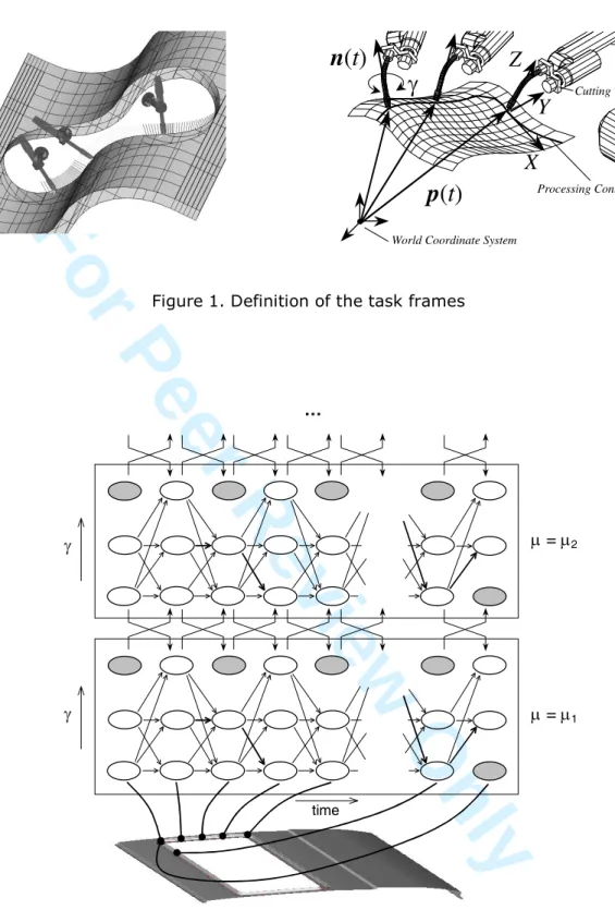
where t is a scalar argument (time); p(t) R3 defines the Cartesian coordinates of the tool tip, and

n(t) R3 is the unit vector of the tool axis direction, which must be normal to the part surface (figure 1). These data can be directly extracted from the graphical model of the part, by defining the processing contour as an “augmented line”. for example. The path is assumed to be closed and

time-uniformly sampled into the sequence of nodes { , ; k 0,...n}

k k n =

p , where the first and the last

coincide ( p₀ = p_n; n₀ = n_n), and the time-interval length is t .

[Insert figure 1 about here]

To describe the tool spatial location, let us also define the Cartesian displacement along the path

;

1 k k

k p p

p = ₊ k = 0,1,2,_Kn 1 and introduce a unit direction vector || ||

k k

k p p

a = , which

is tangent to the part surface and to the direction of the points for the tool motion. For the last node, let us define this vector as a_n = a₀. Then, assuming that the vectors ak and nk are mutually orthogonal, each node may be associated with the Cartesian frame in which the x-axis is directed

1 2 3 4 5 6 7 8 9 10 11 12 13 14 15 16 17 18 19 20 21 22 23 24 25 26 27 28 29 30 31 32 33 34 35 36 37 38 39 40 41 42 43 44 45 46 47 48 49 50 51 52 53 54 55 56 57 58 59 60

For Peer Review Only

along the path, the z-axis is directed along the cutting tool, and the y-axis is computed in such way that these three axes form a right-handed coordinate frame. The corresponding homogenous transformation matrix is 4 4 1 0 0 0 × × = k k k k k k p n a n a H (2)

where “×” denotes the vector product. It should be noted that, generally, the CAD-imported vectors

nk and the computed vectors nk may be slightly non-orthogonal. In this case, it is necessary to

adjust {ak} using the classical Gram–Schmidt orthogonalisation:

|| || ; ) ( T _{k k k k k} k k k a n a n a a a a .

The introduced frame sequence {H_k k = 0,...n} is used as a pivot for defining the complete pose of the robotic tool, which is usually determined by six independent parameters (three Cartesian coordinates and three Euler angles). However, since the cutting tool is axially symmetric, the frames Hk can be rotated around corresponding zk-axes without any influence on the technological

process. This one-dimensional redundancy leads to an infinite set of admissible tool locations described by the matrix product

] , (-, ) ( ) ( = k k k z k k R H L , (3)

where k is an arbitrary scalar parameter and Rz( ) is the standard z-axis rotation matrix.

Another source of redundancy is related to the manipulator posture µ (or the configuration index), which is required for the unique mapping from the task space to the joint coordinate space. So, in total, the robotic task is described by a sequence of locations (3), while the design parameters

are represented by the sequence { k 0,...n}

k ,

k µ = . At this step, the design problem can be

formulated in the terms of non-linear programming; however this straightforward approach is not prudent because of high search space in this problem.

1 2 3 4 5 6 7 8 9 10 11 12 13 14 15 16 17 18 19 20 21 22 23 24 25 26 27 28 29 30 31 32 33 34 35 36 37 38 39 40 41 42 43 44 45 46 47 48 49 50 51 52 53 54 55 56 57 58 59 60

For Peer Review Only

3.2. Constraints

While planning the robot motions for laser cutting and other curve-tracking applications, a designer must take into account three types of constraints: task, robot kinematic and collision constraints (Hwang et al., 1994). Task constrains are expressed in the terms of the tool position/orientation required to perform the assigned task and, for the considered problem, they are described by expressions (3). Robot kinematics constraints are caused by the manipulator geometry and expressed as workspace limits as well as limits on the range the manipulator joint coordinates. And collision constraints arise from the need to avoid collisions between the robot links, workpiece and workcell components.

To define the kinematic constrains more precisely, let us briefly review some results from robot kinematics. For the anthropomorphic serial manipulators that are usually employed with laser cutting, the direct kinematic model, which defines the tool location L corresponding to the joint coordinate vector q , may be always expressed in a closed form, as

base i i i i tool T q T T q L = = 6 1 1 ) ( ) ( , (4)

where i-1Ti is the transformation matrix from the (i-1)th to the ith link, qi is the corresponding joint

coordinate, the matrix Ttool defines the tool tip location with respect to the manipulator mounting

flange, and the matrix Tbase defines the robot base location in the world coordinate system.

Particular expressions for the homogenous matrices i-1Ti for various manipulators can be found in

common reference books (Ceccarelli, 2004; Spong et al., 2006), usually they are expressed using the Denavit-Hartenberg (DH) notation:

4 4 1 1 0 0 0 ) os( ) in( 0 ) in( ) in( ) ( ) ( ) os( ) in( ) os( ) in( ) in( ) ( ) in( ) ( ) ( × = i i i i i i i i i i i i i i i i i i i i d c s q s a s q cos cos q c q s q c a s q s cos q s q cos q T 1 2 3 4 5 6 7 8 9 10 11 12 13 14 15 16 17 18 19 20 21 22 23 24 25 26 27 28 29 30 31 32 33 34 35 36 37 38 39 40 41 42 43 44 45 46 47 48 49 50 51 52 53 54 55 56 57 58 59 60

For Peer Review Only

where ai, di, i are the DH-parameters associated with ith link and ith joint (the offset distance, link

length, and twist angle, respectively).

However, the inverse transformation (from the task coordinates space to the manipulator joint space) is generally non-unique and may not be expressed in a closed form. In practice, robot designers prefer special types of manipulator architecture, which admit closed-form solutions. Otherwise, there exist numerical techniques to deal with this problem (Manocha and Canny, 1994; Pashkevich, 1997; Husty et al., 2007). Within our study, and independent of the solution type (analytical or numerical), the inverse kinematical transformation will be presented in an abstract form as q = f_c1(L,µ), where µ is the configuration index that determines the manipulator

posture, and the set contains all combinations of admissible postures (shoulder right/left, elbow

up/down, wrist plus/minus). For most of 6–axis industrial manipulators, the number of different

configurations is equal to 8, but generally this can rise up to 16 (Manseur and Doty, 1989).

It should be stressed that typical robot controllers do not allow changing the manipulator configuration while mowing between successive nodes and the use of the Cartesian space on-line interpolation (LIN and CIR commands). But for cutting applications, this specific kinematic constraint can be released by temporarily switching to the joint-space interpolation for these specific path segments (PTP command). So, in contrast to our previous work (Pashkevich et al., 2004), here we do not use separate manifolds for each value of µ. This also causes some modifications at the final stage, when the optimal path is translated into a robot control code.

Using the inverse kinematic transformation, the sequence of the admissible tool locations (5) can be mapped onto the joint coordinate space as follows:

{

, k n

}

C_Q = Q_k( _k,µ_k) = f_c1(R_z( _k) H_k, µ) _k (- , ], µ_k =1K (5) considering both the workspace dimension constraints (i.e. inverse kinematics existence) and the joint limits q_imin < q_i < q_imax, i I, I_q ={1,_K6}. For computational convenience, the constraint violation case is denoted as ( ) =

k k

Q (this notation is easily implemented in data structures

1 2 3 4 5 6 7 8 9 10 11 12 13 14 15 16 17 18 19 20 21 22 23 24 25 26 27 28 29 30 31 32 33 34 35 36 37 38 39 40 41 42 43 44 45 46 47 48 49 50 51 52 53 54 55 56 57 58 59 60

For Peer Review Only

employed in optimisation algorithms). Concerning the joint limits, it worth mentioning that the latest laser-cutting manipulators allow unlimited rotation of the 4th and 6th axes, so in this case

5} 3, 2, {1, = q I .

The collision constraints are managed in a similar way, i.e. their violation leads to Q_k( _k) =

and corresponding tool locations are inevitably excluded from a feasible set. The collision detection functions are standard routines of industrial robotic CAD packages, together with the direct/inverse kinematics of the robotic manipulators.

From a practical point of view, the desired path planning algorithm should produce “smooth

motions at reasonable speeds and at reasonable accelerations”. Hence, many of aforementioned

authors impose constraints on the joint torques. However, addressing the torque constraints requires a rather accurate dynamic model, which is problematic in real-life industrial projects. A practical solution consists of transforming torque constraints into acceleration ones using the manipulator specification data provided by the manufacturer.

Within the frames of the discretised path presentation (1), the joint velocity/acceleration constraints may be expressed via the finite-difference approximation as:

) ( 1 v i v k , i k , i q q q < , (6) ) ( 2 1 2 a i a k , i k , i k , i q q q q + < , (7)

where q_i(v) = &q_imax t; q_i(a) = &&q_imax t2; the notations q& and _imax q&& define the maximum ith joint _imax

velocity and acceleration; and v and a are the scaling factors to be adjusted by the designer.

Hence, the complete set of constraints arising from the technical nature of the problem are

summarised in inequality ( ) !

k k

Q and in the expressions (6), (7), which ensure the path

existence and its admissible curvature in the joint coordinate space.

1 2 3 4 5 6 7 8 9 10 11 12 13 14 15 16 17 18 19 20 21 22 23 24 25 26 27 28 29 30 31 32 33 34 35 36 37 38 39 40 41 42 43 44 45 46 47 48 49 50 51 52 53 54 55 56 57 58 59 60

For Peer Review Only

3.3. Design objectives

In the qualitative terms, the desired manipulator motion should be as smooth as possible while satisfying the contour-tracking and actuator-dependent constraints (7) - (9). This means that the qualitative performance measures should be based on some type of the “smoothness” and

“economy” measures applied to all manipulator joints (Edan and Nof, 1997; Shoval et al., 1998).

For the considered problem, which is based on the discrete path presentation, the degree of smoothness can be evaluated by the following criteria:

• total displacement ( )

_%

= = n k i,k k k i,k k k s i q q J 1 1 1 1 ) , ( -) , ( ) , ( µ µ µ , (8)

• maximum increment (speed) ( ) ) , ( -) , ( ) , ( 1 1 1 = _{i,k k k i,k k k} k v i max q q J µ µ µ , (9) • coordinate range ( )

[

]

[

]

) , ( ) , ( ) , ( _{i,k k k} k k k k , i k i max q min q J µ = µ µ , (10)

where i is the joint number, and , µare the vectors composed of the design parameters 0, 1, … n and µ0, µ1, …µn respectively.

A geometrical explanation of these performance measures is the following. The displacement criterion evaluates the total amount of joint motions (without regard to the direction of the motion). The increment characterizes the coordinate variation during the time-interval t and is proportional to the speed. Finally, the range evaluates the extent of the coordinate variation during the motion.

Intuitively, the minimization of each of these criteria should lead to a smoother generated path. However, as follows from related studies, the objectives (8) – (10) may be in competition with each other, i.e. minimizing one of them may degrade the performance in others. Besides, these assessments are computed for each joint coordinate. Thus, the resulting performance measures form a vector. The designer must choose one of the techniques that are usually used for multi-criteria problems (Steuer, 1985; Cheng and Shih, 1997; Ehrgott , 2005).

1 2 3 4 5 6 7 8 9 10 11 12 13 14 15 16 17 18 19 20 21 22 23 24 25 26 27 28 29 30 31 32 33 34 35 36 37 38 39 40 41 42 43 44 45 46 47 48 49 50 51 52 53 54 55 56 57 58 59 60

For Peer Review Only

In this paper, instead of giving preference to a particular criterion or optimisation technique, all the following options are admitted: (i) defining priority of partial objectives or the primary objective; (ii) applying minimax technique, i.e. the worst-case optimisation; (iii) assigning weights to combine multiple criteria in a linear function. Independent of the chosen option, the corresponding vector-optimisation engine must include the scalar-optimisation routines that are developed in the following section.

4. Path planning algorithm 4.1. Search space discretisation

A practical method to obtain an optimal (or feasible) solution under the constraints described in sub-section 3.2 is the sampling of the allowable domain for the redundant parameter . Such an approach transforms the continues search space into an acyclic directed graph, with the vertices uniquely representing the matrix of the tool location L and the vector of joint coordinates Q.

Let us assume that the parameter [- , ] is sampled with the step = 2 /m0, m0 Z and, for

each discrete value of and each admissible configuration µ , the locations (5) are tested for

kinematic and collision constraints. Then, the admissible locations, which satisfy the constraints, are included in the search space in such manner that each Cartesian-path node {pk, nk} produces

several elements of the data structure {L, Q}:

U

k m j k,j j , k k k 1 , } { = () * + , -. _QL n p (11)

where mk is the number of the successful locations for the kth node. It should be noted that the

“path-smoothness” constraints (6), (7) are not tested at this stage yet, since they are associated with several successive locations. The test result can be presented in the plane t×( , µ), where the abscissa (index k) corresponds to the time t, and the ordinate (index j) corresponds to the combination of the redundant parameter and the configuration index µ (see figure 2).

[Insert figure 2 about here] 1 2 3 4 5 6 7 8 9 10 11 12 13 14 15 16 17 18 19 20 21 22 23 24 25 26 27 28 29 30 31 32 33 34 35 36 37 38 39 40 41 42 43 44 45 46 47 48 49 50 51 52 53 54 55 56 57 58 59 60

For Peer Review Only

Under such assumptions, the feasible search space can be represented by a directed graph with the vertices

U

U

k m j k,j j , k n k V 1 0 = = () * + , -= Q L (12) and edges

U

U

U

₁1 1₁ 1 1 = = = () * + , -( ) * + , -= k m l k ,l l , k j , k j , k k m j n k , E Q L Q L , (13)

which connect only successive tool locations from the entire set (5). Hence, the considered path-planning task is reduced to the following network optimisation problem.

Design Problem. For given set of vertexes V and set of edges E, find the “best” path of length n

/( / ) * /+ / , -. /( / ) * /+ / , -. /( / ) * /+ / , -= 0 n j , n n j , n j , j , j , j , n j j j _Q L Q L Q L K K 1 1 1 1 0 0 0 0 1 0, , ) ( (14)

with initial and final states

U

0₁ 0₀ 0 m j ,j j , V = () * + , -Q L and

U

n m j n,j j , n n V 1 = () * + , -Q L ,

which minimizes a specified performance index.

It should be stressed that, in this formulation, both the initial and final states are not unique, but the problem can be transformed to the classical problem by adding the virtual start and end nodes. Besides, the initial and the final states may not coincide with each other, as it follows from the technical nature of the problem. It is also worth mentioning that all nodes are solvable for the inverse kinematics and admissible for the collision tests (otherwise they are excluded from the graph (V,E) at the stage of the graph generation).

To solve this network optimisation problem, it is also necessary to define the distance matrix, which assigns certain lengths to the graph edges. Since in the Cartesian space the tool path is sampled uniformly, the distance should be based on a joint space metric. While defining this metric, it is necessary to take into account that the actuator capacities (i.e. maximum speed, acceleration,

1 2 3 4 5 6 7 8 9 10 11 12 13 14 15 16 17 18 19 20 21 22 23 24 25 26 27 28 29 30 31 32 33 34 35 36 37 38 39 40 41 42 43 44 45 46 47 48 49 50 51 52 53 54 55 56 57 58 59 60

For Peer Review Only

etc.) are different for different manipulator axes. So, the displacement components qi

corresponding to the joint displacement vector, which are q = ( q₁,_K q₆), should be weighted. The most appropriate way of assigning the weights, is using the maximum axis speed q&_imax

specified by the manufacturer. In this case w_i = &(q_imax t)-1and the product w_i q₁ shows the degree of actuator capacity utilisation with respect to speed. Finally, combining the evaluations for all axes, the distance in the joint space may be defined using the Euclidean, Manhattan or Chebychev metrics (Deza, 2006) that are usually used because of both the computational convenience and their clear physical meaning (Pashkevich et al., 2004):

%

= = 6 1 2 ) ( ) ( i i i E q w q 2 ;

%

= = 6 1 | | ) ( i i i M q w q 2 ; ( ) max| _{i i}| i C q = w q 2 (15)

While applying the above expressions, it is necessary to consider that for cutting applications, the 4th and 6th axes may allow unlimited rotation. In this case, before computing the distance 2(.), the differences

i

q must be minimised in accordance with the following expression:

{

+ 2

}

{4, 6} = min q p , i q i Z p i (16)

where p is an integer number. For example, for the axes 1, 2, 3, 5, the movement from q_i(k)= 120°

to q_i(k+1)=+120° corresponds to the joint coordinate displacement q_i= 240+ °. However, for the axes 4 and 6 it is equal to q_i= 120° and the target joint coordinate is must be changed to

° = + 240 ) 1 (k i

q . In practice, there is an open question: which metrics of 2_E(.),2_M(.),2_C(.), should be chosen? So, it is proposed to give some freedom to the designer and to include the choice of the corresponding option in the set of parameters for the optimisation algorithm.

4.2. Generation of optimal path

Since there is no combinatorial optimisation technique, which is able to solve this multi-objective problem directly, the vector performance measures (8) - (10) should be converted into an aggregate scalar criterion. At this step, a relevant metric is applied to the sequence of the path

1 2 3 4 5 6 7 8 9 10 11 12 13 14 15 16 17 18 19 20 21 22 23 24 25 26 27 28 29 30 31 32 33 34 35 36 37 38 39 40 41 42 43 44 45 46 47 48 49 50 51 52 53 54 55 56 57 58 59 60

For Peer Review Only

segments whose length is computed using one of the expressions (15). Hence, the desired scalar

criteria may be based on the non-weighted Manhattan/Chebychev norm. The weights wi, which are

used for calculating the segment distance 2(.), are altered between optimisation runs to produce a set of Pareto-optimal solutions.

Corresponding expressions for the objective functions may be written as follows:

(

)

%

= = n k a k k s j k j k J 1 1 ) ( ) , 1 ( -) , ( ) , ( µ 2 Q Q (17)

(

( , )- ( 1, )

)

) , ( 1 ) ( ₌ k k a k k j k j max J µ 2 Q Q (18)

where 2_a(.), a {E, M, C} is the distance function, the notation jk defines the values of the redundant parameters , µ at the kth node and, for further convenience, the vectors of the joint coordinates Qk,j are denoted as Q(k,j).

For the additive objective J , an optimal path can be found by means of dynamic (s)

programming. This is a standard shortest-path problem in an acyclic directed graph. Nevertheless due to the graph specific properties (node clustering), it is not reasonable to apply known algorithms (Dijkstra's , Bellman-Ford, etc.).

This problem is also closely related to the generalised travelling salesman problem (GTSP) employed in the motion and process planning for which there are some efficient optimisation routines, see for example (Ben-Arieh et al., 2003; Dolgui and Pashkevich, 2006).

To describe the proposed algorithm in terms of graph theory, let us introduce the following notations. Let G = (S₀ U S₁UKS_n, E) be an acyclic directed graph with the set of vertices

k n k S V 0 =

= U partitioned into n+1 mutually exclusive and exhaustive subsets (clusters)

} ..., 1

{ _{kj k}

k v , j , m

S = = of sizes | S_k |= m_k. Here v_kj = (k,j) denotes the jth vertex of the kth cluster.

It is assumed that each edge (u,v) E is evaluated by some travelling distance 2( vu, ). The clusters must be visited in a strictly predefined order

n

S S

S . ._K.

1

0 , passing via exactly one vertex in

1 2 3 4 5 6 7 8 9 10 11 12 13 14 15 16 17 18 19 20 21 22 23 24 25 26 27 28 29 30 31 32 33 34 35 36 37 38 39 40 41 42 43 44 45 46 47 48 49 50 51 52 53 54 55 56 57 58 59 60

For Peer Review Only

each cluster. It should be noted that the above formulation does not admit cluster intersection (i.e.

l k , S

S_{k I l} = 4 ! ). This is in agreement with usual engineering practices.

For such a formulation, a vertex may be coded as pair (k, j), an edge is identified by quadruplet (k1, j1, k2, j2), and the solution is defined by the array of j-indices {Jopt(k), k=0,1,…n} of the sequential visiting vertices. Also, following this notation, the cluster sizes are defined in the array {Jmax(k), k=0,1,…,n} and the cost of the edges are denoted as 2(k1, j1, k2, j2).

A basic expression for the developed algorithm is derived in the following way. Let us consider a reduced order sub-problem with k clusters S0, S1, … Sk-1, and let d_k5 _1,j be the length of the shortest path S₀ . S₁ ._K. S_{k 1} that links a vertex v_{k 1,j} S_{k 1} to the nearest vertex u S₀ , assuming that all the clusters are visited exactly once. Then, using the dynamic programming, the optimal solutions for the sub-problem with k+1 clusters S0, S1, … Skcan be found by choosing the best edge

) ,

(u v_k,j , u S_{k 1} that links the vertex v_k,j S_k with the cluster Sk-1 :

{

d v v

}

, k , , n min d j , k p , k p , k p j , k = 1 + ( 1 , ) =12K 5 5 ₂ (19)

Therefore, the desired solution for n+1 clusters S0, S1, … Sn can be obtained sequentially, starting from k = 0 with d₀5_,j = 0,4j , successively increasing the k-index up to n, computing d_k5_,j , and, finally, choosing the smallest value among

n j

,

n , j , , m

d5 =12_K . The corresponding sequence of

the j-indices { } 1 0 5 5 5 n j , j ,

j _K , which defines the shortest path, is extracted in reverse order, starting

from k = n and 5 = { _n5_,j}

j n argmin d

j .

An outline of the path planning procedure based on this technique is presented below. The procedure consists of five basic steps where the first two, (1) and (2), implement the recursion (19). These steps deal with creating matrices of optimal distances Mdist(k,j) and the corresponding matrix

Mind(k, j) of the optimal j-indices of the preceding clusters. In steps (3) and (4), the minimum value

in the nth column of the distance matrix Mdist(.) is computed, in order to select the best vertex in the

1 2 3 4 5 6 7 8 9 10 11 12 13 14 15 16 17 18 19 20 21 22 23 24 25 26 27 28 29 30 31 32 33 34 35 36 37 38 39 40 41 42 43 44 45 46 47 48 49 50 51 52 53 54 55 56 57 58 59 60

For Peer Review Only

last cluster. Finally, in step (5), the best vertices of the preceding clusters are iteratively extracted from the matrix Mind(.) to generate the optimal path described by the array of the optimal indexes

Jopt(.). The procedure also uses the array Jmax(.) containing the upper range for the j-index and the

vertex distance function 2(.) defined previously. The notation d6 defines the infinity (or the largest

number for computer implementation).

Procedure: Path planning (dynamic programming) (1) For j = 1 to Jmax(0) do

Set Mdist(0, j) := 0; Mind (0, j) := 0

(2) For k = 1 to n do

For j = 1 to Jmax(k) do

(a) Set dmin := d6

(b) For p = 1 to Jmax(k-1) do

( ) Set dcur := Mdist(k-1, p) + 2(k, j, k-1, p)

(7) If k > 0 & fv(k, j, p) ! 0

Set dcur := d6

( ) If k > 1 & fa( k, j, p, Mind(k-1, p) ) ! 0

Set dcur := d6

(8) If dcur < dmin then

Set dmin := dcur; jopt := p

(c) Set Mdist(k, j) := dmin; Mind(k,j) := jopt;

(3) Set dmin := inf;

(4) For j := 1 to Jmax(n) do

(a) Set dcur := Mdist(n, j)

(b) If dcur < dmin then

Set dmin := dcur; jopt := j

(5) For k = 0 to n do

Set Jopt(n-k) := jopt; jopt:= Mind(n-k, jopt);

A distinct feature of the developed procedure, which takes into account the problem-specific requirements, is contained in sub-steps (2b7) and (2b ) that verify the path-smoothness constraints (6) and (7). Sub-step (2b7) incorporates the function f_v(k,j,p), which evaluates the velocity constraints (6) for all manipulator axes while the manipulator moves from the location Lk-1,p to the

location Lk,j (a non-zero value of this function corresponds to violating one of the velocity

constraints). Similarly, at the sub-step (2b ), the function f(k,j,p,l)

a verifies the acceleration

constraints (7) for the location sequence Lk-2,l , Lk-1,p , Lk,j , where the location Lk-2,l is assumed to be

1 2 3 4 5 6 7 8 9 10 11 12 13 14 15 16 17 18 19 20 21 22 23 24 25 26 27 28 29 30 31 32 33 34 35 36 37 38 39 40 41 42 43 44 45 46 47 48 49 50 51 52 53 54 55 56 57 58 59 60

For Peer Review Only

the optimal predecessor of Lk-1,p, i.e. l = M_ind(k-1,p). It is obvious that this is a penalty-function

approach. The definition of the path-segment of the double length strictly corresponds to the

optimality principle incorporated in dynamic programming.

The computational complexity of this algorithm is quite acceptable for practical applications. It is evaluated as O(n m2), where n is the number of clusters and m is the maximum cluster size. This estimation also includes the calculation of the cost components. This calculation is executed for the neighbouring clusters only.

A similar algorithm can be applied for the minimax design objective J( ). The only

modification needed deals with the sub-step (2b ), which must be re-written in accordance with the following expression:

{

d v v

}

, k , , n max min d _{k ,p k ,p k,j} p j , k = 1 ; ( 1 , ) =12K 5 5 ₂ (20) that is also based on the dynamic programming principle. Combining two of the path generation options (objectives J and (s) J( )) and altering the distance metrics weights wi together with the

constraint weights v and a (see expressions (6) and (7) ), the designer can generate a collection of

the candidate solutions to be included in the Pareto-optimal set.

4.3. Generation of control programs

As assumed in previous sections, the sequence {nk, pk}, describing the tool path in the Cartesian

space, is extracted from the CAD workpiece model by uniformly sampling the cutting contour. In performing such a conversion, the designer must specify an appropriate distance S between nodes, which should be small enough to ensure desired accuracy of the contour approximation. However, during off-line programming, there exists a lower bound on the time-sampling step, which is determined by the control unit parameters. Let us examine this problem in detail.

In industrial robots, the control code describes the sequence of the path segments (with a specified interpolation type within each: linear/circular for Cartesian space and linear for joint space). Some advanced robot controllers implement also spline interpolation. It is obvious, that for

1 2 3 4 5 6 7 8 9 10 11 12 13 14 15 16 17 18 19 20 21 22 23 24 25 26 27 28 29 30 31 32 33 34 35 36 37 38 39 40 41 42 43 44 45 46 47 48 49 50 51 52 53 54 55 56 57 58 59 60

For Peer Review Only

tracking the cutting contour, the Cartesian space interpolation is used the most, while the joint space interpolation is utilised only for travelling through a singularity.

To reduce the control program size, see for example (Korb and Troch, 2003), the intermediary nodes within the line/circular segments are not specified. Instead, they are generated on-line using the trapezoid velocity profiles that typically include three sections (acceleration, uniform motion, and deceleration). Their duration depends on the desired displacement and the velocity/acceleration constraints imposed on both each joint variable and on the Cartesian coordinates. Moreover, in the continuous motion mode (i.e. without stopping at the end of the segment), the successive segments are joined in such way that the acceleration section of the succeeding segment coincides with the deceleration section of the preceding one. As a result, the velocity is maintained at the same level for all three time sections.

However, for short segments, the trapezium reduces to a triangle. In addition, the travel time for each section is sampled using the controller “clock time” and is rounded up to a greater value. Therefore, for very short distances, the basis of the triangle (time) is fixed while its height (velocity) is adjusted, to ensure the square be equal to a specified displacement. Thus, the joining of very short segments yields unexpected velocity reduction, which is not admissible for the considered technological equipment.

To eliminate this effect, the distance between the successive nodes must be not less than

min min v

S = 9 , where v is the cutting speed, and 9min is the minimal duration of the

acceleration/deceleration sections. In practice, the value of S_min is high enough to be considered

during robot programming. For example, for typical industrial case studies (cutting speed 10 m/min; clock time 0.005 ms; at least 4 time-samples per acceleration section) the minimal distance between the nodes is equal to 3.3 mm. At the same time, in the model (1) the cutting contour is usually sampled with a step less then 1 mm.

To comply with this constraint on the inter-node distance, it is necessary to aggregate short segments into straight and circular portions, which are suitable for on-line implementations. This

1 2 3 4 5 6 7 8 9 10 11 12 13 14 15 16 17 18 19 20 21 22 23 24 25 26 27 28 29 30 31 32 33 34 35 36 37 38 39 40 41 42 43 44 45 46 47 48 49 50 51 52 53 54 55 56 57 58 59 60

For Peer Review Only

problem is solved using our heuristic algorithm, which is based on the sequential extracting of maximum-length sub-sequences with a fixed initial point that can be approximated by a straight or circular line within given tolerances.

At each run, the algorithm deals with three nodes: p(ks), p(km) and p(ke) , where ks, km and ke are

the indices of the start, middle and end nodes of the current segment, respectively. Within the search loop, the index ke is successively increased from the initial value k_s+2 and the middle index

km is recomputed as k_m = (k_s + k_e)/2 , where . denotes the integer part. Then, each current path segment is verified for its capability to the line and circular approximation:

(1) if the angle between the vectors p(k_m)- p(k_s) and p(k_e)- p(k_m) is less than max ,

then the segment admits a straight-line approximation, and the index ke is increased.

(2) if the radius of the circle defined by the points p(k_s), p(k_m) and p(k_e) is less than Rmax ,

then the segment admits a circular approximation, and the index ke is increased.

(3) otherwise, the segment enlargement is stopped and the last accepted triple (k_s,k_m, k_e) defines the extended segment of the linear or circular type (commands LIN and CIR).

This loop is then repeated for the rest of the nodes, assigning new values for the indices

2 + = = _{e e s}

s k;k k

k , etc. However, before applying this algorithm, the node sequence is divided into

the sections with the same configuration index µ, and the subsequent sections are connected by the arcs using joint-space interpolation (command PTP). The length of the connecting segment must be also greater or equal to S_min, so this segment is successively expanded in both directions.

For each segment, the motion arguments (tool locations in the Cartesian or joint space) are defined by the node L(ke) for the LIN/PTP commands, and by the pair {L(ke), L(km)} for the CIR

command. It should be noted, that at this stage there is no need to modify the joint angles for the 4th and 6th axes, which admit unlimited rotations (this procedure is executed by the controller on-line).

As a result, for the specified tolerances max and Rmax , the optimum path with the uniform short

sampling step S is aggregated into longer sections, which are described by the robot control

1 2 3 4 5 6 7 8 9 10 11 12 13 14 15 16 17 18 19 20 21 22 23 24 25 26 27 28 29 30 31 32 33 34 35 36 37 38 39 40 41 42 43 44 45 46 47 48 49 50 51 52 53 54 55 56 57 58 59 60

For Peer Review Only

commands (LIN, CIR and PTP , with required location arguments) and may be reproduced on-line by a robot controller with the desired Cartesian velocity.

5. Efficiency of the developed technique

5.1. Case-study: robot motion planning for 2D cutting

To demonstrate the efficiency of the proposed technique, first let us apply it to the planar cutting performed by a Scara robot, which possesses a 1 d.o.f. redundancy with respect to this task. The geometric/kinematic parameters of the manipulator are as follows: the link lengths are l1 = l2 = 1000

mm; the tool offset (horizontal) is d = 250 mm; the maximum speed of the axes involved in the planar motion is 120, 120, and 320 deg/sec, respectively. The cutting contour is a square

800 mm× 800 mm with rounded angles (radius 100 mm). Its centre is located at point (1000 mm,

1000 mm) and is surrounded by and an obstacle described in detail in (Pashkevich et al., 2004). After the sampling, the contour is presented as a set of 60 uniformly distributed nodes (this corresponds to the cutting speed 30 m/min, sampling distance 50 mm, and sampling time 0.1 sec).

The direct kinematic model of this manipulator is described by the equations

3 2 1 2 1 2 1 1 2 1 2 1 1 ) ( ) ( ) ( ) ( ) ( ) ( q q q sin d q q sin l q sin l y cos d q q cos l q cos l x + + = + + + = + + + = : : : , (21)

where q1, q2, q3 are the joint coordinates, and x, y,: are the tool location parameters (two Cartesian

coordinates and an orientation angle). It should be noted that one of the joint coordinates (vertical translation of Scara manipulator) is not included in the model, since the z-axis motion is not redundant for the considered planar task.

To derive the inverse kinematic model, let us define x₀= x dcos(:); y₀= y dsin(:) and sequentially solve the obtained equations for q2, q1 and q3:

2 1 2 2 2 1 2 0 2 0 2 _{2 ll} l l y x cos a q = µ + ; 2 2 0 2 2 1 0 2 2 0 2 2 1 0 1 _{( )} ) ( 2 q sin l x q cos l l y q sin l y q cos l l x tan a q = +₊ + (22) 2 1 3 q q q =: (23) 1 2 3 4 5 6 7 8 9 10 11 12 13 14 15 16 17 18 19 20 21 22 23 24 25 26 27 28 29 30 31 32 33 34 35 36 37 38 39 40 41 42 43 44 45 46 47 48 49 50 51 52 53 54 55 56 57 58 59 60

For Peer Review Only

where µ= sgn(q2) is the configuration index.

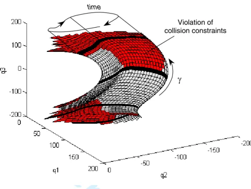
Using the inverse model and altering the tool orientation : with the step of 10o, a set of 1385 feasible tool locations {Lk,j} and the corresponding set of joint coordinates {Qk,j} have been

generated. To detect collisions, both the manipulator and the obstacle were described by a set of line segments. Then, all pairs from these sets were examined for intersections. The obtained manifold of the admissible motions is presented in figure 3, where the forbidden regions (with detected collisions) are shaded. Within the frames of this geometrical interpretation, the problem is to find the best closed path on the manifold surface, which encloses this figure and avoids the forbidden region. Another interpretation of the problem is given in figure 4, where the admissible and forbidden tool locations are shown in the set of the ( , t)-planes and the goal is to find the best route from the left to the right vertical lines. It should be noted that, in spite of the apparent simplicity of the last interpretation, the optimisation problem is essentially complicated by the non-Euclidian distances.

[Insert figures 3, 4 about here]

For the considered robotic task, a set of solutions was obtained. These solutions are presented in tables 1 & 2 and differ by both the optimisation criteria and the weights: wi, v and a. For each

partial criterion, there are given the best values of single-objective optimisations (in brackets). As the tables show, for the relaxed velocity/acceleration constraints, tuning of the weights wi can barely

produce acceptable results. Most of the solutions have a tendency for oscillations in the orientation axis, which is undesirable in practice.

In contrast, the explicit imposing of constraints on the velocity and acceleration (and adjusting

corresponding weights v , a) simplifies obtaining smooth solutions with the balanced values of

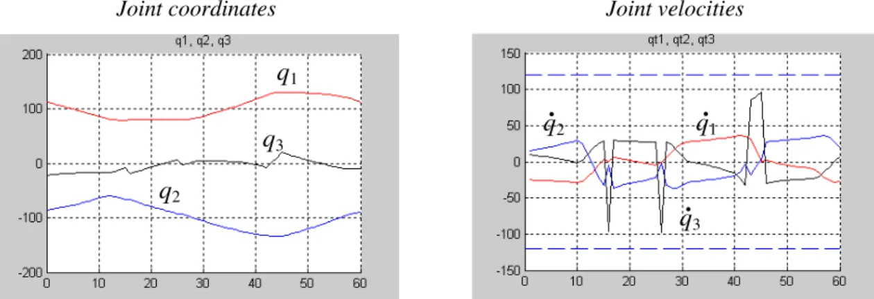
the partial criteria. This result is illustrated in figures 5 and 6, which contain the trajectories generated for the weights w (qmax t)-1

i

i = & . They also demonstrate rather high oscillation of q3 for

the unconstrained case (see figure 5; joint velocity plots) and very smooth trajectories for the

1 2 3 4 5 6 7 8 9 10 11 12 13 14 15 16 17 18 19 20 21 22 23 24 25 26 27 28 29 30 31 32 33 34 35 36 37 38 39 40 41 42 43 44 45 46 47 48 49 50 51 52 53 54 55 56 57 58 59 60

For Peer Review Only

constrained optimisation (similar plots in figure 6). Hence, the proposed approach gives the possibility to eliminate oscillations in the orientation axes.

[Insert Tables 1, 2 about here] [Insert figures 5, 6 about here]

The final comparison of the obtained results can be done using a multi-axes plot which presents two typical solutions with the values of nine partial design objectives J_1v, J_2vKJ₃ (see figure 7). The first solution (a) corresponds to the best result of a known technique, which corresponds to the very tedious adjusting of the weights wi. The second solution (b) was generated straightforwardly,

using the developed method with the standard values w_i = &(q_imax t)-1 and with a very fast and simple tuning of the algorithm parameters v and a. As follows from the comparison, the developed

technique reduces essentially oscillations of the orientation axis (see axes J3s, J3v and J3 in figure

7, where relevant performance measures are lower by the factors 2…3), while maintaining almost the same values for the rest of the objectives.

[Insert figure 7 about here] 5.2. Comparison with other techniques

The main advantage of the proposed technique compared to the previous work (Pashkevich et al., 2004) is the ability to generate a smooth path without the tedious adjusting of weights wi. This

useful feature is achieved by modifying the standard dynamic programming routine: including an implicit verification of the velocity/acceleration constraints while creating the backtracking matrix. From this perspective, the new technique is robust with respect to weights assigned by the designer. This advantage has been confirmed by a number of industrial projects where the developed technique has been successfully applied.

Another advantage, which was demonstrated by several 3D cutting case-studies, relates to the algorithm’s ability to generate a robot path with large rotations of the manipulator orientation axes (more than 360°). This allows the exploitation of recent advances in the kinematics of cutting

1 2 3 4 5 6 7 8 9 10 11 12 13 14 15 16 17 18 19 20 21 22 23 24 25 26 27 28 29 30 31 32 33 34 35 36 37 38 39 40 41 42 43 44 45 46 47 48 49 50 51 52 53 54 55 56 57 58 59 60