HAL Id: hal-01788421
https://hal.archives-ouvertes.fr/hal-01788421
Submitted on 5 Mar 2019
HAL is a multi-disciplinary open access
archive for the deposit and dissemination of
sci-entific research documents, whether they are
pub-lished or not. The documents may come from
teaching and research institutions in France or
abroad, or from public or private research centers.
L’archive ouverte pluridisciplinaire HAL, est
destinée au dépôt et à la diffusion de documents
scientifiques de niveau recherche, publiés ou non,
émanant des établissements d’enseignement et de
recherche français ou étrangers, des laboratoires
publics ou privés.
Rheological parameters identification using in-situ
experimental data of a flat die extrusion
Nadhir Lebaal, Stéphan Puissant, Fabrice Schmidt
To cite this version:
Nadhir Lebaal, Stéphan Puissant, Fabrice Schmidt. Rheological parameters identification using in-situ
experimental data of a flat die extrusion. AMPT’2005 -8th International Conference on Advances in
Materials and Processing Technologies, May 2005, Gliwice-WIsla, Poland. 4 p. �hal-01788421�
Rheological parameters identification using In-situ experimental data of a flat die extrusion
N. Lebaala, S. Puissanta, F.M. Schmidtb
a Institut Supérieur d’Ingénierie de la Conception, Equipe de Recherche en Mécanique et Plasturgie 27 rue d’Hellieule, 88100 Saint-Dié-des-Vosges, France
b
Ecole des mines d’Albi Carmaux, Laboratoire CROMeP, Campus Jarlard- Route de Teillet 81013 Albi Cedex 9, France
Abstract
Viscosity is an important characteristic of flow property and process ability for polymeric materials. A flat die was developed and brought into service at Maillfer[8], to make rheological characterizations. Measurements were made with two different slit heights, at different extrusion speeds, for one type of material (LDPE). In this paper, the optimization by response surface method, with the moving least squares approximate (MLS) [5-6], is used to identify the rheological parameters of thermoplastic melt. The objective is to minimize the difference between the measurement pressure obtained in flat die and the numerical pressure calculated by one dimensional finite difference programme by sections [1].
Global relative error between these both pressure is the objective function. This objective function is minimised by varying the rheological parameters. For this minimization two methods are used i.e. local response surface and global response surface. The rheological parameters obtained by these methods allow calculating the viscosity, validated by comparing an experimental viscosity measured on a capillary rheometer.
Keywords: MLS; Numerical Simulation; Identification of rheologicals parameters; Extrusion;
1. Introduction
The defects of extrusion (like the weld-lines, the bad distribution, a fairly uniform exit velocity distribution throughout the extrusion, problems of stagnation zones) are influenced by the geometry of the die of extrusion, the operating conditions such as temperature of regulation, flow rate and the rheological parameters of melt. In order to eliminate these problems we propose to determine a sufficiently robust method of optimization to be applied in industry. In a first step, in order to validate the method of optimization, we will identify the rheological parameters (behavior of the pseudo plastic melt) of the plastic melts starting from the points of measurement obtained in flat die.
A standard extruder at various flow rates feeds the flat die and two series of tests were carried out, with two thicknesses of die to cover a sufficient range to make rheological characterizations.
In spite of various utilities of plastics, the knowledge and the control of their behaviours remains always approximate.
Physicists tried to characterize the properties of these materials, thus wanting to reproduce their behaviours using a simple or complex model. A number of viscosity
Corresponding author.
E-mail address : [email protected]
models have been published, such as the well-known Power-law model, Ostwald–Waele model, Cross model, and Carreau model, and so on. These models are established on the basis of some types of fluid. Ji-Zhao Liang [10] he investigated the melt viscosity in steady shear flow of several polymers by employing a capillary rheometer and the characteristics of shear viscosity. K. Geiger and H. Kuhnle[2] used a empirical correlation between density, pressure and temperature to identify a rheological parameter.
Our objective is to identify the rheology of a plastic melt directly from on-line production because that saves us much time and money, because in this way we will not be obliged to make measurement on dies capillary standard.
For that we will identify the rheological parameters, using algorithm of optimization named as response surface method, with the moving least squares approximate [5 -6], and can obtain approximation by using the design of experiments [3].
2. The optimization benchmark
The flat die is equipped with 4 pressure transducers, spaced 100 mm apart; however only the pressure difference between the first and last transducer was considered for the analysis. A first series of tests has been performed with the flat die. Measurements were made
with two different slit heights at different extrusion speeds for one type of material (LDPE). The experimental data is used as listed in table 1.
Table 1.
Experimental data slit 5 and 10mm Q [Kg/h] T [°C] ? P[bar] ? [Kg/m 3 ] h [mm] 11,2 166 53 779 5 60 175 99 779 5 143 192 125 773 5 239 210 138 767 5 10,9 185 12,7 779 10 69,2 195 26 772 10 189,5 210 34,3 761 10 339,5 229 36,7 755 10
Conductivity k=0.115 Watt/°C m Specific heat Cp=1.90e03 K joules/°C m3
Fig. 1. Geometry of the Flat die
the geometry of the die is W = 100 mm, L = 300mm. Ltotal=500 mm. The thickness (h) of the die remains
constant for a test, but it can be changed by taking in to account the correction factor (h/L)[1].
3. Numerical simulation parameters
The measurement of viscosity cannot be obtained directly because the shear rate is unknown and the three parameters for the power-law. On the other hand, three physical parameters related to viscosity such as pressure, temperature and the flow rate are directly measurable. We will use a one-dimensional calculation programme by sections of finite difference method [1], to calculate the variation of pressure with power-law for each point of measurement. Choice of this geometry by taking in to account the Correction factor[1] 0.1 and 0.05 as a function of the thickness to width ratio, h/W.
4. Design variables and objective functions
The power-law is defined as:
1 m T 1 0e K
(1) There are three variables (K, m and ß) for a power law with a thermal dependence of the Arrhenius type.
The objective function is the difference between the measured pressures and calculated pressures obtained by simulated program of finite difference method.
The objective of this simulation is to determine the rheological parameters K, m and ß which makes it possible to minimize the difference between the calculated pressures and the experimental pressures. We chose as variable optimization the rheology of the polymer and the objective function represents the value of the sum of the variations of the calculated pressures and experiment pressures for each point of measurement. J=( npm((pexp pcal)/pexp)2). (2)
5. Optimization procedure
5.1. Choice of algorithm
The algorithm of optimisation must be carefully chosen when one single analysis requires several hours of CPU time. Nondeterministic or stochastic methods such as Monte-carlo method and genetic algorithm [7] can obtain global minimum but they need a lot of evaluations for the functions to converge. Decent methods require the computations, the gradients of the functions, such as BFGS[9] with ought constraints, and SQP[8] based on
Lagrangian methods, it can be shown that the solution of the nonlinear equality constrained optimization problem.
The computation of gradients by finite difference is time consuming and depends on the perturbed parameters. For the above reasons we decided to consider a response surface method.
5.2. Response surface method
The method of response surface consists the construction of an approximate expression of objective function starting from a limited number of evaluations of the real function.
The main idea is to approximate the objective function through a response surface. To obtain a good approximation we used a moving least square method. In this method, the approximation is computed by using the evaluation points by design of experiments around the locus where the value of the function is needed.
6. Moving least-squares approximation
We will use moving least-squart interpolations that are used to approximate response surface of objective function. Let the dependent variable bef(x)in the domain S and the approximation of ~f(x).
P1
h
W
P2
L
) x ( a ) x ( p ) x ( f ~ T
(3) The nodes are defined by x1,…..xn where xI=(xI,yI) in
2D, xI=(xI,yI,zI) in 3D;
Where p (x) is a polynomial basis and aT(x)is the vector of coefficients. The polynomial basis of order 2 in two dimensions is given by
2 2 1 2 2 1 i 1(x) (y) (x) (x)(y) (y) P (4)
In the moving least-square interpolation, at each point x, a is chosen to minimize the weighted residual:
2 T i i(f P(x) a(x)) w ) a ( J ) Pa F ( ) Pa F ( ) a ( J 21 (5)
wher
w
i is a weight function, such that w is non-zero over a limited support or domain of influence and is non-increasing over.To find the coefficients, we obtain the extremum of J(a) by 0 ) a ( J'
So we have Z . B Q ) x ( a 1
(6) where WP P Q T
(7) and WQ P B T (8)
Z is the dependent variable.
7. Local response surface:
This method is based on traditional minimization by the algorithm of fig2, with use of a local response surface of variable in each point. We fixed a step of grid at 0.01* X0.
X0 is the initial value of the variable of optimization
The initial values are: K0=12000, m0=0.641370 and
ß0=1078 °K, we used a uniform local grid i.e. “Design of
experiments”
The constraints for the variables of optimization K, m and are respectively, 400 < K < 20000, 0.01 < m <1 and 500 < ß < 3000 °K for the first constraint, and n*P
for the second constraint, with P is the step of the grid and n is the number of points of grid.
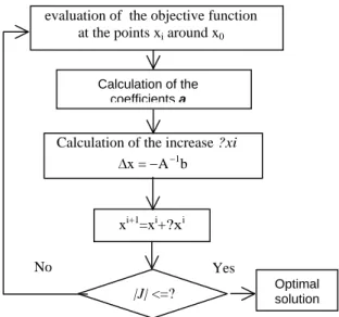
Fig. 2. Flowchart of the optimisation
The iterative process stops when the successive points are superpose with a certain tolerance.
8. Global response surface
The objective of this technique is to search for the global minimum on the field domain, the constraints is similar to the first constraints in local response surface method. Initially, in first iteration we constructed a grid of 5*5*5 points (125 points) for a global approximation, then to each iteration we constructed grid of 3*3*3 (27 pints) for the local approximation.
9. Results
9.1. Result of local response surface:
Figure 3 represents the evolution of the objective function and figure (4), (5) and (6) represents respectively the evolution of the coefficients of the law of rheology K, m and during the process of optimization. The optimal solution, which represents the minimal variation between the pressures obtained by finite difference calculation and the measured pressures,
In iterations 20, the value of the function objective obtained is 8.e-5 , with K= 9826.14, m= 0.4179 and ß = 1553.41, a time CPU is 1hours 42minutes, on a machine Pentium IV, 2.4 GHz, 512 Mo RAM, the results of the pressures are presented in table 2.
Optimal solution
Yes No
Calculation of the increase ?xi b A x 1
xi+1=xi+?xi
evaluation of the objective function at the points xi around x0
Calculation of the coefficients a
Fig.3. Convergence of the objective function (result for the local method)
Fig.4. Evolution of B during the process of optimization (result for the local method)
Fig.5. Evolution of m during the process of optimization (result for the local method)
Fig. 6 evolution of ß during the process of
optimization (result for the local method)
We can choose between the precision and the time computing, for example in iteration 10 we obtained an error of 6.848 e-3 with a time CPU 51 minute, the values of the coefficients of rheology are: K=10562, m=0.4304, ß = 1131 °K.With iteration 15 we obtained an error of 5.2 e-4, with a computing time of 1hours 16minutes in the same machine, the coefficients obtained are: K=10077, m= 0.4239, ß= 1350 °K.
0
20
40
60
80
100
120
140
0
50
100
measurements pressures Calculat pressureFig.7. Experimental and Calculated pressures with parameters determined by method 1
J Iteration K Iteration m Iteration ß Iteration P re ss u re s b ar Pressures bar
10 100 1000 10000 100000 1 10 100 1000 10000 Capillary rheometer T=170 Capillary rheometer T=210 Capillary rheometer T=250 optimization T=170 optimization T=210
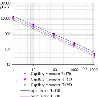
Fig. 8. Calculated and measured viscosity
9.2. Result of global response surface:
The solution is obtained after 6 iteration with a precision of 8.4e-3 and a time computing CPU of 1hours 13minutes on a machine Pentium IV, 2.4 GHz, 512 Mo RAM. Fig 9 represents the evolution of the function objective and fig 10, 11 and 12 represent respectively the variables of optimization K, m and . The optimum parameters are: K=10213, m= 0.4064, ß=1386.2617 °K.
Fig. 9. Convergence of the objective function (results for the global method)
Fig. 10. Evolution of K during the process of optimization (result for the global method)
Fig. 11 Evolution of m during the process of optimization (result for the global method)
Fig. 12. Evolution of ß during the process of (optimization result for the global method)
s-1 Pa. s J Iteration K Iteration m Iteration ß Iteration
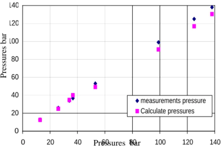
0 20 40 60 80 100 120 140 0 20 40 60 80 100 120 140 measurements pressure Calculate pressures
Fig.13. Experimental and calculated pressure with parameter determinates by method 2
10 100 1000 10000 10 100 1000 10000 Capillary rheometer T=170 Capillary rheometer T=210 Capillary rheometer T=250 optimization T=170 optimization T=210
Fig. 14 Calculated and measured viscosity
10. Comparison of the two methods:
We remarked in the table (2) that the solution obtained by the method (1) local response surfaces is more precise but with a more increased computing time where the difference in time between both methods is 30 min. On the other hand the global response surface method (2) avoided local minimum and we can also improve by varying the design of experiments and the method of approximation to optimize the computing time CPU. Table 2. Results of optimization h [mm] Q [Kg/m3] T [°C] ? P [bar] ? P[bar] local (1) Residue n (1) ? P[bar] global (2) Residue n (2) 5 3,9e-6 166 53 52.11 2.8e-4 49.32 4.8e -3 5 2,1e-5 175 99 96.69 5.4e-4 91.03 6.4e -3 5 5,1e-5 192 125 121.6 7.3e-4 116.8 4.3e -3 5 8,6e-5 210 138 132.9 1.3e-3 130.4 3e -3 10 3,8e-6 185 12.7 12.49 2.7e-4 12.48 3e -4 10 2,4e-5 195 26 25.15 1.e-3 24.89 1.8 e -3 10 6,9e-5 210 34 34.69 1.2e-4 34.66 3.7 e -4 10 1,2e-4 229 36.7 39.27 4.9e-3 40 8.1 e-3
10.1. Pressures
The figures (7), (13) illustrates the difference between the measured pressures and calculated pressures obtained by rheogical parameters. Which are identified by optimization using response surface method. It is noticed that there is almost no variation, which means that our method is very robust and gives very good results for the two approximations global and local.
10.2. Viscosity
We remarked well in the graph of viscosity obtained by the coefficients found by response surface method fig (8), (14), that it does not have an error between the points of measurements obtained in capillary rheometer and viscosity obtained by the method of optimization except in the zone that has high shear rate. As we have no knowledge of the inlet temperature so we used a simplification where we gave the same temperature of exit as of inlet temperature, on the other hand at this level of shear rate the polymer is reheated and this
simplification is not completely right, but the variation between viscosities is always less important.
11. Concluding remarks
We can have the conclusion that since we obtained good results by the response surfaces method (global and local), so this allows us to know the rheology of a plastic directly in series of production and that saves us much time and money, because this way we will not be obliged to make measurement on standard capillary dies.
s
-1Pa . s
P re ss u re s b ar Pressures barWith this method we can find out the rheology of polymer starting from the true geometry even if this geometry is complex, by measurements of pressures, flows rate and the temperatures, we can determine the rheology of the material used.
12. Prospects
We have tried another method of approximation for approximating well the global response surface using the Krigeage method, which made it possible to approximate the global objective function, and saves us much computing time.
Using response surface method to optimize the geometry of die extrusion using calculate program 3D “ REM3D® ”
Acknowledgments References
[1] J. F. AGASSANT, P. AVENAS. J.-PH. SERGENT, P. J. CARREAU «Polymer rocessing. Principles and Modeling». Hanser Publishers, 1991.
[2] K. GEIGER ; H. KUHNLE. « Analytische Berechnung einfacher Scherstromungen aufgrund eines Fliebgesetzes vom Carreauschen Typ», Rheogica Acta, Vol.23, p355-367,1984.
[3] JACQUES GOUPY « Plans d’expériences pour surfaces de réponse». », Industries Techniques, série conception Dunod, Paris 1999
[4] D. Schlafli «Filière rhéométriques théorie/filière plate » Rapport interne de NOKIA MAILLEFER, 1997.
[5] K. M. LIEW, Y. Q. HUANG, J. N. REDDY «Vibration analysis of symmetrically laminated plates based on FSDT using the moving least squares differential quadrature method 2003. [6] Y. KRONGAUZ, T. BELYTSCHKO. «Enforcement
of essential boundary conditioned in mesh less approximations using finite elements ».Computer methods in applied 1996.
[7] J. M. RENDERS. «Algorithmes génétiques et réseaux de neurones ». Hermès, Paris, 1995. [8] B. Horowitz, S. M. B. Afonso. « Quadratic
programming solver for structural optimisation using SQP algorithm » Advance in engineering software, p 669-674, 2002.
[9] J. L. Morales « A Numerical study of limited memory BFGS methods» Applied Mathematics Letters, p 481-487, 2002.
[10] J-Z Liang “Characteristics of melt shear viscosity during extrusion of polymers” Polymer Testing p 307-311, 2002