HAL Id: hal-02547591
https://hal.archives-ouvertes.fr/hal-02547591
Submitted on 20 Apr 2020HAL is a multi-disciplinary open access archive for the deposit and dissemination of sci-entific research documents, whether they are pub-lished or not. The documents may come from teaching and research institutions in France or
L’archive ouverte pluridisciplinaire HAL, est destinée au dépôt et à la diffusion de documents scientifiques de niveau recherche, publiés ou non, émanant des établissements d’enseignement et de recherche français ou étrangers, des laboratoires
Model Checking and Parameterized Distributed Systems
Isabelle Vernier
To cite this version:
Isabelle Vernier. Model Checking and Parameterized Distributed Systems. [Research Report] lip6.1997.011, LIP6. 1997. �hal-02547591�
Model Checking and Parameterized Distributed Systems
Isabelle Vernier LIP6, Université Paris 6
4 place Jussieu, 75252 Paris - Cedex 05, France email : [email protected]
tel : (33 1) 44 27 71 04, fax : (33 1) 44 27 62 86
Abstract: We propose a solution to solve part of the verification problem for a set of parallel programs that are the instantiations of a same algorithm. The instantiated parameter is the number of processes. All the possible programs are supposed to satisfy the same properties. Petri nets with guarded transitions model the programs. The originality of our method is to build a symbolic graph that allows us to verify temporal properties that concern the behavior of the whole program as well as properties that concern the behavior of a single process. The nodes of the symbolic graph are predicates that represent sets of states.
Key Words:Verification, validation, temporal logic, parameterized systems, Petri nets
I. Introduction
Many distributed systems are designed with a finite but unknown number of processes. They are required to have similar behaviors whatever the number of processes is. A straightforward way to verify their properties is to instantiate the program with the desired number of processes. The verification has to be performed again if the number is changed. A solution is to develop verification methods that are independent of the value of the parameter. In [1] and [16], the authors prove the undecidability of the whole problem. Several solutions have been proposed that solve parts of it. They consider systems with one parameter, the number of identical processes sharing a finite and defined number of resources managed by a control process.
The methods that are proposed in [5, 6, 9, 14, 20], have strong restrictions on the properties that can be verified, are not automatic or are automatic but not complete. All these methods need to represent the set of reachable states of a particular system. Unfortunately, although a state graph is built, no representation of the reachable states of the instantiated systems is given. The solution we propose in [18] avoids this drawback. It is an automatic but not complete method. We build a finite symbolic graph that represents all the reachable states and executions of all the instantiated systems. The nodes of the graph are predicates that represent sets of states. Properties verification is performed on this graph. To obtain this result we do not identify the processes.
We present two extensions of our method. The first one is the extension of the class of distributed systems we can study. We allow the evolution of a process to be dependent on the states where the other processes are. The second extension overcomes drawback of our method. As we do not identify the processes, we cannot verify properties that concern the behavior of a single process. If we consider a mutual exclusion protocol, we can prove that once a process asks for the critical section, a process, not necessarily the same, will enter it. We cannot prove starvation-free properties. We present here the way to extend our method to verify such properties. As all the processes have the same behavior, it is sufficient to prove the property for a single one whose identity is not important.
To build the reachability graph of a system we need to have a formal representation of it. The systems we consider are modeled by means of Petri nets with guarded transitions. The guards represent conditions on the number of tokens in some places. They allow us to realize our first extension. For the second extension, we use the idea of the colored Petri nets. To follow the execution of a process we have to particularize the token we associate with it. Therefore, we only modify the representation of states. The execution of an action is independent of the kind of the tokens. It depends only on the states where the tokens are.
In Section 2 we introduce the model we use to represent the systems. The predicates are presented in Section 3. In Section 4 we show how the symbolic graph is built. Section 5 concerns the verification of properties. We conclude in Section 6 and present further works.
II. Formal Model
We represent parallel systems by means of Petri nets with guarded transitions because of their well-known expressive power [13]. Guards allow us to test the value of the number of tokens among several places.
II.1. Petri nets and basic notations
We use Petri nets that are extended with guarded transitions. Definition 1 Guarded Petri nets
A guarded Petri net is a 5-tuple, PN = <P, T, Guard, Pre, Post> where:
- P is a set of places, T is a set of transitions, P ∩ T = Ø and P ∪ T ≠ Ø,
- ∀t ∈ T, Guard(t) is a function from NP to {true, false}. Guard(t)p denotes the value to which place p is compared. If it equals -1 it means that the guard defines no condition on place p.
- Guard(t) = [Pt≤ n] or Guard(t) = [Pt≥ n], n ∈N and Pt⊆ P ∀p ∈ Pt, Guard(t)p = nelse Guard(t)p = -1
or Guard(t) = true (default value). ∀p ∈ P, Guard(t)p = -1 - Pre, Post are functions from P × T to N. Notation
We extend the functions Pre and Post to sequences of transitions. Let p be a place, s = t1,…, tm be a sequence of transitions
Pre(p,s) =
∑
i=1 mPre(p,ti) and Post(p,s) =
∑
i=1 mPost(p,ti).
Definition 2 Guarded State machine
A guarded state machine is a guarded Petri net <P, T, Guard, Pre, Post> with: ∀t ∈ T, ∃p1 ∈ P, Pre(p1,t) = 1 and ∃p2 ∈ P, Post(p2,t) = 1,
∀p ≠ p1, Pre(p,t) = 0 and ∀p ≠ p2, Post(p,t) = 0. Definition 3 Markings
A marking m is a function from P to N that defines a state of the Petri net. It associates with each place the number of tokens it contains. The initial marking represents the initial state of the Petri net.
Definition 4 Value of a guard
• Guard(t) = [Pt≤ n], Guard(t)(m) = true iff ∑ p ∈ Pt
m(p) ≤ n • Guard(t) = [Pt≥ n], Guard(t)(m) = true iff ∑
p ∈ Pt
m(p) ≥ n • Guard(t) = true then Guard(t)(m) = true.
Definition 5 Enabled transition
A transition t is enabled for a marking m, m[t>, iff: ∀p ∈ P, m(p) ≥ Pre(p,t) and Guard(t)(m) = true. Definition 6 Firing rule
A marking m' reached from m after the firing of a transition t, m[t>m', is computed as follows: ∀p ∈ P, m'(p) = m(p) - Pre(p,t) + Post(p,t).
II.2. Distributed systems with parameter
We consider distributed systems with one parameter, the number of processes. As in [2, 5, 9, 11, 14, 15, 20] all the processes are identical, i.e., they have similar behaviors independent of their identity. They communicate by shared resources. A control process manages the accesses to the resources.
The behavior of the identical processes is represented by a guarded state machine. The control process and the resources are represented by a Petri net.
Definition 7 Distributed system
A system with n identical processes and a control process is represented by a guarded Petri net <P, T, Guard, Pre, Post> where:
• P = Pp∪ Pc, Pp∩ Pc = Ø
Pp represents the states of the identical processes, Pc represents the states of the control process and the resources.
• T = Tp∪ Tc,
Tp represents the actions of the identical processes, Tc represents the actions of the control process.
Τhe transitions t of Tp∩ Tc represent the accesses to resources. • ∀t ∉ Tp, Guard(t) = true.
The guards concern only the actions of the identical processes. • <Pp, Tp, Guardp, Prep, Postp> is a guarded state machine where
Guardp, Prep, Postp are the restrictions of Guard, Pre, Post to the transitions of Tp and places of Pp.
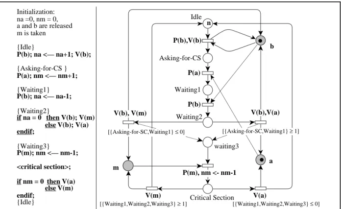
We illustrate this paper with a mutual exclusion algorithm defined by Morris [12]. It presents a starvation-free mutual exclusion algorithm with a finite number of semaphores. A process "takes" a semaphore with a P action and "releases" it with a V action. The algorithm needs three semaphores a, b and m. The semaphore a protects the accesses to the variable nm and the semaphore b protects the accesses to the variable na. They are used to ensure the starvation-free property of the algorithm. We can see that it is not necessary to explicitly represent these two variables. Each of them counts the number of processes that are in some states. We replace these variables by guards but we have to keep the semaphores to respect the semantic of the algorithm. The semaphore m protects the accesses to the critical section. Figure 1 gives the algorithm and the model with a Petri net. We have put together actions whose execution in an atomic way does not modify the properties of the algorithm (if the first action of the sequence is
executable, so is the sequel of the sequence). This allows us to reduce the number of intermediate states.
Initialization: na =0, nm = 0, a and b are released m is taken {Idle} P(b); na <— na+1; V(b); {Asking-for-CS } P(a); nm <— nm+1; {Waiting1} P(b); na <— na-1; {Waiting2} if na = 0 then V(b); V(m) else V(b); V(a) endif; {Waiting3} P(m); nm <— nm-1; <critical section>; if nm = 0 then V(a) else V(m) endif; {Idle} Idle n Asking-for-CS Waiting1 Waiting2 waiting3 Critical Section P(b),V(b) P(a) P(b) V(a) [{Waiting1,Waiting2,Waiting3} ≤ 0] V(m) [{Waiting1,Waiting2,Waiting3} ≥ 1] m b a V(b), V(m) [{Asking-for-SC,Waiting1} ≤ 0] V(b),V(a) [{Asking-for-SC,Waiting1} ≥ 1] P(m), nm <- nm-1
na represents the number of processes in places Asking-for-CS and Waiting1 nm represents the number of processes in places Waiting1, Waiting2, Waiting3
Figure 1 : Morris Algorithm
III. Sets of markings
The algorithms to build state graphs of Petri nets, as coverability graph [8], symbolic graph of colored Petri nets [3], reduced graphs [17], suppose that the initial markings of the net is completely defined, i.e., the value of the parameter is fixed. To build a graph independently of this value, we define elementary predicates that characterize sets of markings. They are equivalence classes that bring together markings regarding the marked places, the enabled transitions and the way they are reached. The nodes of the symbolic graph are elementary predicates.
The initial elementary predicate determines the initial configurations of the Petri net that are studied. Part of the gathering of markings is performed while computing the symbolic graph.
III.1. Predicates
The initial elementary predicate characterizes the initial states of the instantiated systems we want to study. The number of tokens in each resource or control place is known. For the guarded state machine we know that the number of tokens is finite and the places where tokens are. We do not know the exact number of tokens in each place.
The introduction of two kinds of predicates has been motivated by the firing rule. The application of the firing rule on an elementary predicate leads to a predicate. A predicate can be split into elementary predicates.
A predicate expresses conditions on the number of tokens in each place of a net. The predicates we consider allow us to express the minimum or the exact number of tokens in a
place. In addition, we use a variable to distinguish a process among the identical ones. This distinction allows us to follow the execution of a process. As its distinction does not give it a particular behavior, the properties verified by this distinguished process are verified by all the identical processes.
First we define predicates since they are more intuitive than elementary predicates and independent of the structure of the Petri net. A part of the information given by the predicates concerns the processes apart from the distinguished one, the other part concerns the distinguished one. A variable X represents the distinguished process. We explicitly give the place where it is.
Definition 8 Predicate
- Let P = {p1, …, pn} be a set of places, a predicate pred is defined as:
pred = {p1 op1 x1∧ … ∧ pn opn xn; X in pk} where opi∈ {=, ≥}, xi∈N and pk ∈ P. - A marking m belongs to the equivalence class defined by pred iff:
∀i ≠ k, m(pi) opi xi and m(pk) opk xk+1.
The set of markings defined by the equivalence class pred is noted set[pred].
The set of markings represented by a predicate allows us to define an inclusion relation between predicates. This relation may not respect the place where the distinguished process is. Therefore we can have redundant predicates regarding the set of markings they define but different regarding the place where the distinguished process is. To overcome this problem, we define an inclusion relation taking into account this aspect of the predicates.
Example 1 Redundant predicates
Consider the two following predicates: pred = {Idle ≥ 1, Asking-for-CS = 1, a = 1, b = 1; X in Idle} and pred' = {Idle ≥ 1, a = 1, b = 1; X in Asking-for-CS}. We can see that set[pred] ⊆ set[pred'] but the distinguished process is not in the same place in the two cases.
Definition 9 Predicate inclusion
A predicate pred = {p1 op1 x1∧ … ∧ pn opn xn; X in pk} is included in a predicate pred' = {p1 op'1 x'1∧ … ∧ pn op'n x'n; X in pj} if and only if:
pj = pk and set[pred] ⊆ set[pred'].
To verify the inclusion between two predicates, we only have to compare the integer and operator associated with each place. We now define the minimal marking represented by a predicate. The comparison between markings is performed on the vectors composed of the number of tokens in a place. The places are ordered.
Definition 10 Minimal marking
Let pred = {p1 op1 x1∧ … ∧ pn opn xn; X in pk} be a predicate, the minimal marking represented by pred, noted mpred is such that:
∀i ≠ k, m(pi) = xi and m(pk) = xk+1. ∀m ∈ set[pred], m ≥ mpred.
The operator "≥" may be compared with the ω defined by Karp and Miller [10] to consider unbounded Petri nets. Our notation is more precise since it defines a lower bound. The introduction of ω is motivated by the unboundedness of the Petri net while the "≥" is due to a change of initial marking. For each marking characterized by a predicate, the exact number of tokens in a place with a "≥" is finite and depends on the value of the parameter. This is because the Petri net that represents the behavior of identical processes is conservative. The number of processes in the whole Petri net is constant whatever the execution is.
A predicate may characterize markings of an instantiated system only if the value of the parameter is big enough to respect the conditions that are expressed. With each predicate we associate a bound that represents the minimal possible value of the parameter. This bound determines the instantiated systems that are concerned by a predicate.
Definition 11 Bounds of the parameter
Let pred = {p1 op1 x1, …, pn opn xn; X in pk} be a predicate, the lower bound associated with the parameter is B(pred) = ∑
i=1 n
xi + 1.
Now we define the condition that the parameter of an instantiated program must satisfy to define instances that have markings that can be characterized by a given predicate.
Definition 12 Predicate and instantiated systems
Let pred = {p1 op1 x1, …, pn opn xn; X in pk} be a predicate then pred characterizes markings of systems instantiated
• with at least B(pred) processes if ∃i with opi = "≥", • with exactly B(pred) processesif ∀i, opi = "=". III.2 Elementary predicates
An elementary predicate is a restriction of the predicates that ensures that:
(1) all the markings characterized by an elementary predicate have tokens in the same places,
(2) the same transitions are enabled from the markings characterized by the elementary predicate.
To ensure (2), we first need to define a function Limit that associates with each place the maximum value to which its marking is compared to determine the enabled transitions. If there are, in a place, fewer tokens than the Limit value, it is necessary to know the exact number of tokens in the place. This function allows us to consider the guarded Petri nets. As the Limit of a place is greater or equal to one, we can ensure that if no tokens are in a place, the associated operator is "=". Otherwise the place and its associated arcs can be removed from the net. This ensures (1).
Definition 13 Limit function
Let <P, T, Guard, Pre, Post> be a guarded Petri net, Limit is a function from P to N such that:
∀p ∈ P, Limit(p) = M t ∈ T
ax (Guard(t)p, Pre(p,t))
Definition 14 Elementary predicate
P = {p1, …, pn} be the set of places of a Petri net, pred = {p1 op1 x1, …, pn opn xn; X in pk} is an elementary predicate iff:
- if opi = "≥" then xi≥ Limit(pi). (it ensures (2) and (1))
To test the transitions enabled for the markings characterized by an elementary predicate the same procedure as for a marking is applied. We say that an elementary predicate enables the transitions. We differentiate two cases of enablement: the one that concerns the distinguished process and the others. If a transition is enabled by the distinguished process, we say it is X-enabled.
Definition 15 Enabled transitions
Let pred = {p1 op1 x1, …, pn opn xn; X in pk} be an elementary predicate, a transition t is (X-)enabled for pred, pred[t>, iff:
-∀i≠k, xi≥ Pre(pi,t) and Guard(t)(mpred) = true, - xk≥ Pre(pk,t) (then t is enabled),
- Pre(pk,t) = 1 (then t is X-enabled).
The restriction "if opi = "≥" then xi ≥ Limit(pi)" of the elementary predicate definition ensures that a transition is (X-)enabled for an elementary predicate if and only if it is enabled for all the markings it characterizes.
Property 1 Let pred be an elementary predicate and t a transition. Transition t is enabled for pred if and only if t is enabled for all the markings characterized by pred.
Proof Sketch We use the following facts: - if opi = "≥" then xi≥ Limit(pi),
- ∀pi, ∀t, Limit(pi) ≥ Pre(pi,t) and Limit(pi) ≥ Guard(t)pi. III.3 Splitting of predicates into elementary predicates
The splitting of a predicate appears in the symbolic firing rule. In a predicate, the operator "≥" may be associated with a place even if the minimal number of tokens is less than the Limit value. The splitting procedure allows us to characterize the same set of markings with a finite number of elementary predicates.
Definition 16 Principles of the splitting of a predicate Let pred = {p1 op1 x1, …, pn opn xn; X in pk}
For each place pi such that xi < Limit(pi) and opi = "≥" we compute m (= Limit(pi)-xi+1) new predicates predk that differ from the split one only on the attributes associated with place pi:
∀k, 0 ≤ k < m, opki = "=" and xki = xi + k, opmi = "≥" and xmi = Limit(pi).
At each step the splitting procedure is applied on all the new predicates computed at this time.
A predicate is split into a finite number of elementary predicates. A marking may be characterized by only one of the reached elementary predicates.
Property 2 Let pred be a predicate and pred0, …,predn the splitting of pred into elementary predicates
a) ∀i, j, i≠j, set[predi] ∩ set[predj] = Ø,
b) ∪
i = 0 n
set[predi] = set[pred].
Proof Sketch We use the following facts verified after a step of the splitting
a) the conditions on the number of tokens in the place responsible of the splitting, in the predi, are disjoint.
b) the union of the conditions on the number of tokens in the place responsible of the splitting in predi is equal to the condition in pred. The conditions on the other places are the same in pred and in each predi.
Example 2 Splitting of a predicate
Let pred = {p ≥ 1, q ≥ 0, r = 2; X in r} be a predicate and suppose that Limit(p) = 2 and Limit(q) = 1, then pred is not an elementary predicate. First we split pred regarding p. We obtain the two following predicates:
pred0 = {p = 1, q ≥ 0, r = 2; X in r}, pred1 = {p ≥ 2, q ≥ 0, r = 2; X in r}.
We now split each predi regarding q. We obtain the four following elementary predicates: pred00 = {p = 1, q = 0, r = 2; X in r}, pred01 = {p = 1, q ≥ 1, r = 2; X in r},
pred10 = {p ≥ 2, q = 0, r = 2; X in r}, pred11 = {p ≥ 2, q ≥ 1, r = 2; X in r}. As we have obtained elementary predicates, we stop here the splitting.
IV. Symbolic graph
The building of a symbolic graph by using the symbolic firing rule may lead to infinite graphs even if the graphs of the instantiated systems are finite. We add rules to avoid the building of infinite branches.
IV.1. Symbolic firing rule
The symbolic firing rule defines the elementary predicates that characterize the markings reached from an elementary predicate after the firing of a transition. It is composed of two steps: the firing rule and the splitting of the predicate (if needed). As for the enabling we consider the firing and the X-firing, depending on the process that executes the action.
Definition 17 Symbolic firing rule
Let pred = {p1 op1 x1, …, pn opn xn; X in pk} be an elementary predicate, t a transition that is enabled for pred:
- the predicate pred' = {p1 op'1 x'1, …, pn op'n x'n; X in pk} reached from pred after the firing of a transition t, pred[t>pred', is computed as follows:
∀pi∈ P, x'i = xi - Pre(pi,t) + Post(pi,t), op'i = opi, - if pred' is not an elementary predicate, it is split. t is X-enabled for pred:
- let pj be the place of Pp (set of places that represent states of identical processes) such that Post(pj,t) = 1 (the process that executes the actions moves from place pk to pj)
- the predicate pred' = {p1 op'1 x'1, …, pn op'n x'n; X in pj} reached from pred after the X-firing of a transition t, pred[X-t>pred', is computed as follows:
∀i ≠ k,j x'i = xi - Pre(pi,t) + Post(pi,t), op'i = opi, x'k = xk and x'j = xj;
- if pred' is not an elementary predicate, it is split.
With the symbolic firing rule only and exactly all the reachable markings are computed. Let pred be an elementary predicate that enables a transition t, the symbolic firing rule computes only and exactly all the markings from those represented by pred after the firing of t. If the reached predicate is split, conditions on the number of tokens in the places responsible of the splitting allow us the characterize for each reached elementary predicate the set of their predecessors represented by pred. These conditions are computed, from the reached elementary predicates, by reversing the firing rule.
Property 3 Let pred be an elementary predicate, t a transition and pred0, … predn the elementary predicates reachable from pred after the firing of t.
- ∀m characterized by pred, m[t>m', there is exactly one predi that characterizes m', - ∀m' characterized by one predi,∃m characterized by pred such that m[t>m'. Proof Sketch The proof follows from the firing rule of a Petri net and properties 1 and 2.
The following property is a consequence of both the property 3 and the inclusion relation. Property 4 Let pred and pred' be two elementary predicates, pred ⊆ pred'. Each execution
possible from pred is also possible from pred'. As the inclusion relation takes into account the place where the distinguished process is, the execution we consider can concern the distinguished process.
Proof Sketch The proof follows from the definition of the inclusion relation and property 3. Example 3 Symbolic firing rule
To simplify the notations, in the examples, we do not represent in a predicate the places that contain zero process.
The conditions on the arcs represent the constraints that must verify a marking of the source predicate to have its successor in the target predicate.
Let {idle ≥ 1, a = 1, b = 1; X in Idle} be an elementary predicate. The transition "P(b),V(b)" is enabled and X-enabled. In the second case, it leads to the predicate {idle ≥ 1, a = 1, b = 1; X in Asking-for-CS} that is an elementary predicate. In the first case, it leads to the predicate {idle ≥ 0, Asking-for-CS = 1, a = 1, b = 1; X in Idle} that is not an elementary predicate since Limit(Idle) = 1.
The splitting and the conditions to determine which elementary predicate characterizes the reached markings are shown on Figure 2.
{Idle ≥ 1, Asking-for-CS = 1, a = 1, b = 1; X in Idle} {Asking-for-CS = 1, a = 1, b = 1; X in Idle} {Idle ≥ 1, a = 1, b = 1; X in Asking-for-CS} {Idle ≥ 1, a = 1, b = 1; X in Idle} X-P(b),V(b) P(b),V(b) [Idle = 1] P(b),V(b) [Idle > 1]
Figure 2: (X-)firing of transition P(b),V(b)
The elementary predicate {Asking-for-CS = 1, a = 1, b = 1; X in Idle} characterizes markings of systems with exactly two identical processes (one in state Asking-for-CS and the other in state Idle). The elementary predicate {Idle ≥ 1, Asking-for-CS = 1, a = 1, b = 1; X in Idle} characterizes markings of systems with at least three identical processes (one in state Asking-for-CS and the others, at least two, in state Idle).
The use of the symbolic firing rule to build a symbolic graph may lead to infinite branches that do not represent infinite branches in the reachability graphs of the instantiated systems. These infinite sequences are iterations of a same sequence of transitions. The number of possible iterations depends on the value of the parameters. All the possible iterations are represented in the symbolic graph. As they are in infinite number, i.e., the parameters have no maximal value, they compose an infinite branch. If all the elementary predicates that compose the infinite sequence may be represented by a single one, we can avoid the infinite branch. This possibility depends on properties of the iterated sequence. We have identified a class of sequences for which the reached elementary predicates, after iterations, may be brought together. To respect the definition of elementary predicates, we can bring together only elementary predicates that enable the same transitions. We have to consider the limit values associated with each place. First, we illustrate our solution with the following example.
Example 4 Infinite sequence
Let us consider the following sequence of elementary predicates: {Idle ≥ 1, a = 1, b = 1; X in Idle} [P(b),V(b) (Idle > 1)>
{Idle ≥ 1, Asking-for-CS = 1, a = 1, b = 1; X in Idle} [P(b),V(b) (Idle > 1)> {Idle ≥ 1, Asking-for-CS = 2, a = 1, b = 1; X in Idle} [P(b),V(b) (Idle > 1)> …
The firing of transition "P(b),V(b)", when at least one process is in place Idle, leads from an elementary predicate to the successor in the above list. The iteration of the firing of the transition in the same conditions leads to an infinite sequence. The possibility to iterate the sequence depends on the number of processes that remain in place Idle. It depends on the value of the parameter. Each reached elementary predicate characterizes markings of a system with one more identical process. As Limit(Idle) = 1 and we consider markings with at least one process in place Idle, all the markings characterized by the infinity of elementary predicates can be characterized by a single one:
{Idle ≥ 1, Asking-for-CS ≥ 1, a = 1, b = 1; X in Idle}.
This is due to properties of the sequence composed of the transition "P(b),V(b)". After its execution there is one process less in place Idle, one process more in place Asking-for-CS and all the other processes and resources are in the same place as before the execution.
IV.2. Infinite sequences
A simple comparison between elementary predicates allows us to detect the first elementary predicates of an infinite sequence. The possibility to avoid the infinite construction depends on properties of the sequence of transitions that leads from an elementary predicate to a greater one. We present here a class of sequences that allows us to avoid infinite sequences of elementary predicates.
We define a partial order relation between elementary predicates that allows us to decide if an elementary predicate is greater than another.
Definition 18 Superiority relation
Let pred = {p1 op'1 x'1, …, pn op'n x'n; X in pk} and pred' = {p1 op'1 x'1, …, pn op'n x'n; X in pj} be two elementary predicates. pred is greater than pred', pred ≥ pred', iff:
- pj = pk,
- ∀m ∈ set[pred], ∃m' ∈ set[pred'], m ≥ m', - ∀m' ∈ set[pred'], ∃m ∈ set[pred], m ≥ m'.
An elementary predicate pred is strictly greater than an elementary predicate pred' iff: - pred ≥ pred' and pred ≠ pred' (pred > pred').
As for the inclusion relation, to verify the superiority of a predicate over another one, we only have to compare the integer and operator associated with each place.
The following theorem ensures that the superiority relation allows us to detect all the possible infinite sequences.
Theorem 1
If there is an infinite succession of elementary predicates generated by an infinite sequence of transitions, there are two elementary predicates, pred and pred', and a sub-sequence seq such that pred[seq>pred' and pred' ≥ pred.
Proof Sketch The number of elementary predicates less than or incomparable to another one is in finite number. Two predicates are comparable only if the distinguished process is in the same place. We associate with each predicate {p1 op1 x1, …, pn opn xn; X in pk} a vector
{x1, …, xn, b1, …, bn} with bi = 0 if opi = "=" else bi = 1. We have a partial order among predicates.
We now give a condition that ensures that a sequence of transitions can be iterated only a finite number of times whatever the values of the parameters are. This condition depends on the existence of guarded transitions in the sequence.
Property 5 Let the sequence seq = t1, …, tn, if ∃p and ti, Post(p,seq)-Pre(p,seq) ≥ 1, Guard(ti)=[Pt ≤ n] and p ∈ Pt, the transition seq cannot be iterated an infinite number of times.
Proof Each time the sequence is iterated the number of tokens in place p increases. After a finite number of iterations, the number of tokens in p, before the firing of ti, will be greater than or equal to n.
IV.3. Algorithm
We now define a class of sequences whose iteration leads to an infinite number of elementary predicates that may be characterized by a single one. This is possible since the reached elementary predicates differ by the number of processes in a single place. All the elementary predicates characterize all the possible numbers of tokens greater than a given integer. Therefore, the elementary predicates can be characterized by a single one that characterizes all the possible number of tokens in the place. This is performed by the transformation of an operator "=" into an operator "≥". We name such a sequence: a "state change for one process" sequence. After its execution there is exactly one place with one process less and exactly one place with one process more. The other processes and the resources are in the same place as before the execution. Once the sequence has been executed, if it does not verify property 5, it can be executed again as long as there are at least Limit(state) tokens in the place that loses tokens.
Definition 19 "State change for one process" sequence
Let s = t1 … tm be a sequence of transitions, s is a "state change for one process sequence" iff: ∃p-, Post(p-,s) - Pre(p-,s) = -1, ∃p+, Post(p+,s) - Pre(p+,s) = 1, ∀p ≠ p-,p+, Post(p,s) - Pre(p,s) = 0, ∀i ≤ m, ∀p ∈ P,
∑
j=1 i Post(p,tj) -∑
j=1 i Pre(p,tj) ≥ -1.The last condition ensures that, once the sequence has been executed, it is sufficient to verify that enough processes are in place p+ to decide if it is executable again.
We can now define the rules for the building of the symbolic graph. First we build a symbolic tree. We start from the initial elementary predicate. We compute its reachable elementary predicates. To obtain the graph we identify all the elementary predicates, that are included in another one, with it. This does not modify the set of possible paths and markings (Property 4).
The following rules are applied in the order they are described. We begin to compute the successors of the initial elementary predicate. We continue as long as new elementary predicates are computed. Rules 3 concern the possible infinite sequences. We apply them if an elementary predicate, pred, strictly greater than one of its ancestors, pred', is detected. Rule 3.d is applied when we do not know how to avoid the building of an infinite sequence. We store those markings in a set "Set". Rule 4, applied when no new predicate has to be studied, is a test to
verify that all the predicates of Set are included in other ones that do not belong to Set. In this case, all the possible executions from predicates of Set are represented in a finite way from other predicates. Rules 3.a and 3.b reduce the number of failure cases. Rule 3.a is applied when pred has more operators "≥" than pred'. As the number of places if finite, the number of operators "≥", in a predicate, cannot increase infinitely. We cannot have an infinite sequence of elementary predicates with increasing number of operators "≥". If we continue from pred, we will have to use another rule in a finite time. Rule 3.b is the application of property 5. Rule 3.c concerns "the state change for one process" sequences and detects the failure cases. If a "state change for one process" sequence leads from pred' to pred, we modify pred to represent the set of all the states reachable by executing again the sequence as long as at least Limit(p-) processes remain in place p-. If the number of processes in place p+ is greater or equal to Limit(p+), we change the operator associated with p+ to "≥". Else, we do not modify pred. As some comparisons between tests of 3.b and 3.c are similar we verify property 5 during the test of the "state change for one process" sequence.
Rule 1: We use the symbolic firing rule to compute the elementary predicates successor of a given one.
Rule 2: If we compute an elementary predicate included in one of its ancestors we stop the building of the branch. The reachable elementary predicates are already computed for this branch.
Rule 3: If we compute an elementary predicate, pred, that is strictly greater than one of its ancestors, pred', we examine the sequence s that links the two elementary predicates (we consider the first ancestor that is less than pred):
a) if pred contains more operators "≥" than pred', we continue the building from pred.
b) if s verifies property 5, we pursue the building from pred,
c) else if s is a "state change for one process" sequence we know how to avoid the building
of the infinite branch. We continue the building from the modified elementary predicate.
d) else (s is not a "state change for one process" sequence) Set = Set ∪ {s}. Set is initialized to the empty set.
Rule 4: if each predicate of Set is included in a predicate of the graph (not in Set) we identify the two predicates else we are in a failure case.
The following property ensures that our building algorithm either leads to a finite graph or fails.
Property 6 The algorithm either builds a finite symbolic graph or fails. Proof Sketch We use theorem 1 and property 5 to prove that
- if the graph is infinite, there is an infinite strictly increasing sequence of elementary predicates (Theorem 1),
- we cannot have an infinite strictly increasing sequence of elementary predicates. Rule 3.a and 3.c ensure this fact. As the number of places is finite, the number of operator "≥" in elementary predicates can not increase infinitely,
- the cases 3.d and 4 ensure that if no decision to ensure the building of a finite graph is possible, the algorithm fails.
The symbolic graph can be instantiated if we fix the value of the parameters. For each elementary predicate and for each arc, we can deduce markings and arcs of the reachable graph of the instantiated systems. If in the instantiated system we do not distinguish a process, it is important to see that some elementary predicates are redundant with others. During the instantiation, we have to be careful to not represent twice the same marking or transition.
Definition 20 Instantiated symbolic graph
Let G be a symbolic graph of a Petri net with a parameter, G[n] is the instantiated graph of the Petri net with the parameter equals to n. G[n] is computed as follows:
- for each elementary predicate, pred, of G, we create a node for each marking of the system instantiated by m1, …, ml that is characterized by pred. They are nodes of the instantiated symbolic graph,
- we identify the markings that are the same,
- for each arc, labeled by t, that links two elementary predicates, pred and pred', we create an arc from each marking m characterized by pred, that verifies the condition on the arc, to the marking m' characterized by pred', such that m[t>m'.
Property 7
For all values of the parameter equal to or greater than the lower bound associated with the initial predicate, we can instantiate the symbolic graph.
Proof If the number of processes is greater or equal to the bound associated with the initial predicate, this last one represents the initial state of the instantiated program. Property 3 ensures that markings of the instantiated system are represented in the symbolic graph and the instantiation of the arcs is always possible.
The following theorem ensures that the symbolic graph represents exactly the set of the reachability graphs of all the instantiated systems.
Theorem 2
If the building algorithm does not fail:
- An instantiated symbolic graph is the reachability graph of the system instantiated with the same value,
- The reachability graph of an instantiated system is the symbolic graph instantiated with the same value.
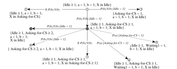
Proof We use properties 1, 3, 7 and that the rule 3 computes all and only reachable states. Example 5 Figure 3 shows first steps of the computation of the symbolic graph.
{Idle ≥ 1, Asking-for-CS ≥ 1, a = 1, b = 1; X in Asking-for-CS ≥ 1} {Idle ≥ 1, Waiting1 = 1, b = 1; X in Idle} {Idle ≥ 1, Asking-for-CS ≥ 1, Waiting1 = 1, b = 1; X in Idle} { Asking-for-CS ≥ 2, a = 1, b = 1; X in Idle} {Idle ≥ 1, Asking-for-CS ≥ 2, a = 1, b = 1; X in Idle} {Idle ≥ 1, a = 1, b = 1; X in Idle} {Idle ≥ 1, a = 1, b = 1;
X in Asking-for-CS} {Asking-for-CS = 1,a = 1, b = 1; X in Idle}
{Idle ≥ 1, Asking-for-CS ≥ 1, a = 1, b = 1; X in Idle} X-P(b),V(b) P(b),V(b) [Idle = 1] P(b),V(b) [Idle > 1] X-P(b),V(b) P(b),V(b) [Idle > 1] P(b),V(b) [Idle = 1] P(a) [Asking-for-CS > 1] P(a) [Asking-for-CS = 1] 1 2 3 4 5 6 7 8 9
Figure 3: Part of the symbolic graph
The elementary predicate 1 represents the set of initial states of all the programs we consider. As the bound associated with this predicate is 2, we study programs with at least two identical processes. The elementary predicate 2 is reached by an action executed by the distinguished process. Elementary predicates 3 and 4 are the result of the splitting of a predicate reached after the execution of action "P(b),V(b)" by a non distinguished process.
Elementary predicate 4 is modified as explain in example 4. From this predicate, the distinguished process can execute action "P(b),V(b)", the reached predicate is the number 7. The other processes can execute actions "P(b),V(b)" or P(a). In these two cases two elementary predicates are reached, 5 and 6 for the first case and 8 and 9 for the second. We see that elementary predicate 5 is included in 4. Therefore, we do not continue the computation of the tree from it. This will be a circuit on the symbolic graph that represents the iteration of the "state change for one process" sequence "P(b),V(b)". A process moves from place Idle to place Asking-for-CS. As long as there is at least one process in place Idle, the reached markings are all represented by elementary predicate 4.
When the building algorithm is finished, we obtain a symbolic graph with 158 nodes and 324 arcs. We can extract from this graph properties of the program whatever the number of processes is (strictly greater than one). It represents the reachability graph of the program instantiated with 8 processes (181 states and 293 arcs) as well as the reachability graph of the program instantiated with 30 processes (2326 states and 4066 arcs). These reachability graphs give information only on the instantiated program. We have no simple way to deduce from the graph for 30 processes the properties of the program with 31 processes. We have to compute a new graph. Our symbolic graph allows us to verify properties of this instantiated program without computing all these states and arcs. The verification is independent of the value of the parameter.
IV.4. Complexity
The complexity of the algorithm to compute a symbolic graph is similar to the one of the algorithm to compute a reachability graph. Let B be the greatest lower bound associated with a predicate of the graph. If a program is instantiated with a number of processes less that B, some of its markings may be explicitly represented by a predicate with no "≥" operator. Therefore, the time used to compute the symbolic graph is equivalent of the sum of the times needed to compute the reachability graphs of the programs instantiated with at most B processes.
V. Verification of properties
In [19] we have presented the algorithms to verify properties on the symbolic graph. The properties are expressed with CTL-X formulas. The graph must sometimes be unfolded during the verification. The unfolding is performed on the elementary predicates. That is because some basic properties may be verified only by some markings represented by elementary predicates. This does not appear when we consider properties that concern only the distinguished process.
We can consider the X operator of CTL, but as we consider properties of the distinguished process, the next state we consider is the next state reached after an action executed by the distinguished process or the control process. We omit the states that represent evolution of an "identical" process. We want to verify properties from the initial state of the program. Because place constraints, we present here only the modifications we have to apply to the CTL model checking algorithm. The model checking algorithm for CTL formulas can be found in [4].
V.1. CTL
Syntax
- {X in p}, where p is a place of the model, is a CTL formula
- If f and g are CTL formulas, then so are ¬f, f ∧ g, f ∨ g, AXf, EXf, A[f U g] and E[f U g].
The notation m |= f indicates that marking m satisfies formula f. The relation |= is defined inductively. We do not present here the rules for the classical logical operators.
Semantics
- m |= {X in p} iff m(p) ≥ 1.
- m |= AXf iff for all markings m' such that ∃t ∈ T, m[t>m', m' |= f - m |= EXf iff for some marking m' such that ∃t ∈ T, m[t>m', m' |= f - m |= A[f U g] iff for all paths (m0 (=m), m1, …),
∃i, i ≥ 0 such that (mi |= g and ∀j, 0 ≤ j < i (mj |= f)) - m |= E[f U g] iff for some path (m0 (=m), m1, …),
∃i, i ≥ 0 such that (mi |= g and ∀j, 0 ≤ j < i (mj |= f))
V.2. Model checking algorithm principles
We want to verify if properties are satisfied by the initial state of the program whatever the number of processes is. The symbolic graph represents all the executions and reachable states of all the instantiated programs. Therefore, it holds all the information needed to verify that a formula is satisfied. Whatever, we have to differentiate two kinds of properties. A formula A[f U g] has to be satisfied by all the executions represented by the symbolic graph. A formula E[f U g] has to be satisfied be at least one execution of each instantiated program. Therefore, when we identify a sequence that satisfies the formula we have to compute the parameter values for which this sequence is executable. The same differentiation has to be considered when we consider "successor state" properties.
The computation of conditions on the parameter values is performed by the computation of the lower bound associated with each predicate of the sequence. To execute the sequence, the number of processes in the program must be greater than or equal to the greatest lower bound if the operator "≥" is associated with at least one place in each predicate. Otherwise, one predicate represents a marking of an instantiated program and the sequence is executable only for this instantiation. The value of the parameter must be equal to the bound associated with the predicate with no "≥" operator. The integers that do not belong to the union of the conditions define the instantiated programs that have reachable states that do not satisfy the expected property.
Another feature due to the symbolic graph is that circuits of the graph are not circuits of the instantiated graphs. They do not represent sequences of transition whose execution does not modify the state of the program. We say they are "false" circuits. The detection of the circuits is essential for the verification of A[f U g] formulas to ensure that it is not possible to have a loop of states that verify f and not g. In our algorithm, when we detect a loop we have to test the sequence of transitions that is associated with it. If it is a real circuit, we have identify markings that do not satisfy the property. Else, we have to follow the verification with the successor states.
Example 6 We present two essential properties of the Morris algorithm: several processes can not be simultaneously in critical section, the algorithm is starvation free. The first property is not a temporal property but it is important. We only have to verify that each predicate satisfies "Critical-Section ≤ 1". The second property can be expressed with a CTL formula that concerns the distinguished process. If each time it wants to access critical section it will access it in a finite time, we can say that the algorithm is starvation free. We have to verify the formula ({X in Asking-for-CS} ⇒ A[true U {X in Critical Section}). The properties verified by the distinguished process are verified by all the identical processes.
By inspection of the symbolic graph, we have verified these two properties. Therefore we can ensure that at each time at most one process is in critical section and Morris algorithm is starvation free. This is true for all instantiated program.
VI. Conclusion
We have presented an algorithm to build a symbolic graph that represents the reachable states of instantiated systems whatever the value of the parameter is. Furthermore we can distinguish a process to follow its behavior to verify properties such as starvation free. A theorem proves that this graph represents exactly all the reachable states of all the instantiated systems and their executions. We have explained how we have to modify the CTL model checker algorithm to verify CTL formulas on the symbolic graph. The CTL formulas we consider concern only the distinguished process. The algorithms to build the symbolic graph and to verify properties are implemented in C language and integrated in the AMI framework [7].
The elementary predicates we consider have the advantage to be easily manipulated. The symbolic firing rule, the splitting operation as well as the verification of superiority or inclusion relations are easy to implement. To extend the set of parallel systems we can study, we may define elementary predicates with a greatest expressive power. We will have to make a choice between the expressive power of elementary predicates and the complexity of the operations on these predicates.
With more expressive elementary predicates, it will be possible to define new sequences of transitions whose iteration leads to elementary predicates that can be characterized by a finite number of elementary predicates.
Another possible extension is to consider distributed systems with several parameters. It is easy to do if we consider programs with several parameterized classes of processes, with constraints on the communication between the processes of several classes to avoid the dependencies between the values of the parameters. A more difficult extension is to parameterized the number of processes as well as the number of resources. The executions of such systems are dependent on relations between these two values.
VII. references
1 Apt K.R., Kozen D.C., "Limits for automatic verification of finite-state concurrent systems", Information Processing Letters, vol. 22:6, pp 307-309, 1986.
2 Balarin F., Sangiovanni-Vincentelli A.L., "On the Automatic Computation of Network
Invariants", Proceedings of Computer Aided Verification: 6th International Conference,
CAV'94, Stanford, CA, David L. Dill (Eds.), LNCS 818, Springer-Verlag, pp 234-246, 1994. 3 Chiola G., Dutheillet C., Franceschinis G., Haddad S., "Stochastic Well-Formed Colored Nets
and Symmetric Modeling Applications", IEEE Transactions on Computers, vol. 42, n° 11, pp 1343-1360, 1993.
4 Clarke E.M., Emerson E.A., Sistla J., "Automatic Verification of Finite-State Concurrent Systems
Using Temporal Logic Specification", , ACM Transactions on Programming languages and
systems, vol. 8, n°2, pp 244-263, 1986.
5 Clarke E.M., Grumberg O., "Avoiding The State Explosion Problem in Temporal Logic Model
Checking Algorithms", Proceedings of the 6th ACM Symposium on Principles of Distributed,
Vancouver, British Columbia, pp 244-303, 1987.
6 Clarke E.M., Grumberg O., Jha S., "Verifying Paramererized Networks using Abstraction and
Regular Languages", Proceedings of the Concur'95, Philadelphia, PA, USA, pp 365-407, 1995.
7 CPN-AMI, "Reference manual, 1.2 version"1994.
8 Finkel A., "A minimal Coverability Graph for Petri Nets", Proceedings of the 11th International Conference on Application and Theory of Petri Nets, Paris, France, pp 233-245, 1990.
9 German S., Sistla A.P., "Reasoning about Systems with Many Processes", JACM, vol. 39, pp 675-735, 1992.
10 Karp R.M., Miller R.E., "Parallel Program Schemata", , Journal of Computer science, vol. 3, n°2, May, 1969.
11 Kurshan R.P., McMillan K., "A Structural Induction Theorem for Processes", Proceedings of the Eighth Annual ACM Symposium on Principles of Distributed Computing, Alberta, Canada, pp 239-247, 1989.
12 Morris J.M., "A starvation-free Solution to the Mutual Exclusion Problem", Information Processing Letter, vol. 8, n°2, pp 76-80, February, 1979.
13 Reisig W., "EATCS Monographs on Theoretical Computer", Ed. Science, Springer Publ. Company, 1985.
14 Rho J.K., Somenzi F., "Automatic generation of networks invariants for the verification of
iterative sequential systems", Proceedings of the 5th International Conference, CAV'93, LNCS
697, Elounda, Greece, pp 123-137, 1993.
15 Shtadler Z., Grumberg O., "Network Grammars, Communication Behaviors and Automatic
Verification", Proceedings of the International Workshop on Automatic Verification Methods
for Finite State Systems, LNCS 407, Grenoble, France, pp 152-165, 1989.
16 Suzuki I., "Proving properties of a ring of finite-state machines", Information Processing Letters, vol. 28, n°4, pp 213-214, 1988.
17 Valmari A., "Stubborn Sets for Reduced State Space Generation", Advances in Petri Nets, LNCS 483, Springer Verlag, pp 491-515, 1991.
18 Vernier I., "Parameterized Evaluation of CTL-X Formulae", ICTLWorkshop, Bonn, Germany, Max-Planck-Institut für Informatik report, MPI-I-94-230, pp 22-31, 1994.
19 Vernier I., "Symbolic Verification of Parallel Programs", rapport de IBP - MASI, n° 95/03, 1995.
20 Wolper P., Lovinfosse V., "Verifying Properties of Large Sets of Processes with Network
Invariants", Proceedings of the Proc.International Workshop on Automatic Verification