HAL Id: hal-01611411
https://hal.archives-ouvertes.fr/hal-01611411
Submitted on 5 Oct 2017
HAL is a multi-disciplinary open access archive for the deposit and dissemination of sci-entific research documents, whether they are pub-lished or not. The documents may come from teaching and research institutions in France or abroad, or from public or private research centers.
L’archive ouverte pluridisciplinaire HAL, est destinée au dépôt et à la diffusion de documents scientifiques de niveau recherche, publiés ou non, émanant des établissements d’enseignement et de recherche français ou étrangers, des laboratoires publics ou privés.
Distributed under a Creative Commons Attribution - ShareAlike| 4.0 International License
complex of the facility
Nicholas John Hutchings, Margit Styrbaek Jorgensen, Ib Sillebak Kristensen,
Jonas Vejlin, Philippe Faverdin, Erwan Cutullic
To cite this version:
Nicholas John Hutchings, Margit Styrbaek Jorgensen, Ib Sillebak Kristensen, Jonas Vejlin, Philippe Faverdin, et al.. Document describing the incorporation into the model complex of the facility. [Con-tract] 9.3, 2014, 44 p. �hal-01611411�
TH
DELIV
Delive
compl
Abstr
adapta decisio focuseDue d
Start d
Organ
ContriAarhu
Jørge
INRA:
Versio
Disse
A
SE
EME 2:
VERABL
erable tit
lex of the
ract:
This ation mea on to foc es on the Fdate of de
date of th
nisation n
butorsus Unive
ensen,
Ib
: Philippe
on: V1
mination
ANI
EVENTH
FOOD,
GranE 9.3
tle: Docu
e facility
s documen asures wa us on the FarmAC meliverable
he project
name of le
ersity: Nic
Sillebak
e Faverd
level:
PU
MA
H FRAM
AGRIC
BIOTE
t agreemeument de
nt describ as include e simple model.e:
M36
t: March
ead contr
cholas Jo
Kristens
in, Erwan
U
LCH
MEWOR
CULTUR
CHNOL
ent numbeescribing
bes how th ed in the farm modAc
1
st, 2011
ractor:
AU
ohn Hutc
sen and
n Cutullic
HAN
RK PROG
RE AND
LOGIES
er: FP7- 26the incor
he ability t modelling delling mctual sub
U
chings, M
Jonas Ve
c
NGE
GRAMM
FISHER
66018rporation
to simulat g complex eans thatmission d
Durat
Margit Sty
ejlin
E
ME
RIES, A
into the
te mitigati x. The st t this docdate:
M40
tion: 48 m
yrbæk
1AND
model
on and trategic cument0
months
Introduction ... 0
FarmAC – model definition ... 1
1 Overview ... 1 2 Agroecological zones ... 3 3 Crop production ... 4 3.1 Energy ... 4 3.2 Carbon ... 5 3.3 Nitrogen/Protein ... 5
3.4 Dry matter lost during processing and storage ... 5
4 Ruminants (cattle and sheep) ... 5
4.1 Intake ... 6
4.2 Maintenance ... 7
4.2.1 Energy ... 7
4.2.2 Protein ... 7
4.2.3 Remobilisation ... 7
4.3 Growth and milk production ... 8
4.3.1 Meat-producing animals ... 8
4.3.2 Dairy animals ... 8
4.4 Carbon ... 9
4.4.1 Mitigation and adaptation measures ... 11
4.5 Nitrogen ... 11
5 Animal housing and manure storage ... 11
5.1 Animal housing ... 12
5.1.1 Bedding and feed waste ... 13
5.1.2 Carbon ... 14
5.2 Nitrogen ... 14
5.2.1 Mitigation measure – low-emission housing, acidification ... 16
5.3 Manure storage ... 16
5.3.1 Carbon ... 17
5.3.2 Nitrogen ... 19
5.3.3 Mitigation measures ... 22
6 Crop and soil ... 22
6.1 Crop production ... 23
6.1 Soil C and N dynamics ... 24
6.1.1 Carbon ... 26
1
6.1 Mitigation and adaptation measures ... 30
7 Farm balances ... 31 7.1 C balance ... 31 7.1.1 C inputs ... 31 7.1.2 C outputs ... 33 7.1.3 Other C flows ... 33 7.2 N balance ... 35 7.2.1 N inputs ... 35 7.2.2 N export ... 35 7.2.3 N balance ... 35 7.2.4 Other N flows ... 36
7.3 Greenhouse gas budget ... 37
8 Appendix I Calculation of air temperature ... 38
9 Appendix II Derivation of the Tier 3 development of N in manure storage ... 40
10 Appendix III Adaptation and initialisation of C-Tool ... 43
10.1 Adaptation ... 43
10.2 Initialisation ... 43
This document describes how the ability to simulate mitigation and adaptation measures was included in the modelling complex. The strategic decision to focus on the simple farm modelling means that this document focuses on the FarmAC model.
A list of the mitigation and adaptation measures is shown in the table below.
Component Measure Target emission
Mitigation
Cattle Nitrate in feed ration Methane
Supplementary fat Methane
Housing Low emission flooring Ammonia
Acidification Ammonia and methane
Manure storage Covering Ammonia
Acidification Ammonia and methane
Anaerobic digestion Ammonia, methane, nitrous
oxide
Field Reduced fertiliser or manure Nitrous oxide, nitrate leaching Cover cropping Nitrate leaching
Low emission fertiliser or manure application
Ammonia
Field acidification Ammonia
Suspension of residue burning
Ammonia, nitrous oxide, black carbon, carbon monoxide
Adaptation
Target effect
Cattle Increased supplementary
feeding
Buffer variations in locally-produced feed
Field Irrigation Drought
Multi-species cropping Production robustness
N fixing crops Production robustness The work was developed during a series of workshops.
The work is reported here in the form of a revised description of the FarmAC model. The revisions relative to Deliverable 9.2 are as follows:
A revised modelling of cattle production.
The addition of the effect of nitrate feeding on enteric methane emission.
The introduction of acidification in animal housing, manure storage and during field application.
The introduction of anaerobic digestion.
A revised method of simulating crop dry matter production. A revised method of simulating nitrate leaching.
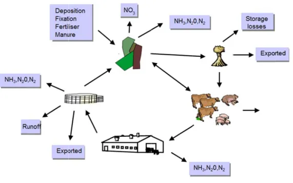
Farm
1 Ov
The obj from fa outputs results a used to enables crop/so can rep categor grazing This all where l housing grazing The flow Figure The flowmAC – mo
verview
jective of th arming syst and losses are expresse o simulate s the model il system is present a sin ies. A lives g animals du lows differ ivestock are g and manu g. ws of carbo 1 Flow ws of nitrogodel def
he model is tems. To d from livest ed as annua flows over l to simulat s defined in ngle field o stock catego uring the gro rences in di e housed fo ure storage on simulated ws of carbo gen simulatfinition
s to simulat o this, the tock, anima al fluxes but a number te changes n terms of a r a whole c ory can app owing seaso iet to be re r part or all is simulate d are as foll on on the far ed are as fo te greenhou model sim al housing ant for the cro of years a in the amo a number o crop rotatio pear more th on and hous eflected in l of the year ed, in addi lows: rm ollows:
use gas emis mulates C an
nd manure op/soil syste
and the res ount of C a f crop sequ on. Livestoc han once on sed animals the produc r, the flows ition to the ssions and n nd N input storage, and em, a simple sults averag and N store uences, whe ck are repre n the farm s for the rem
tion and ex of C and N deposition nitrogen (N ts, transform d fields. Th e dynamic m ged. This a ed in the s ere a crop s esented as l e.g. to desc mainder of t xcretion. O through the n of excreta 1 N) losses mations, he model model is approach oil. The equence ivestock cribe the the year. On farms e animal a during
Figure 2 The mo inputs t investig climate FarmAC dynami housing estimate and N f The mo Fields/c Livesto Manure 2 Flow odel uses a m that should gate a range change or t C is a hybri ic whereas g and manur e changes i flows averag odel takes as crop sequen the sequenc the product whether an soil or burn the amount and whethe the amount sequence, t ock the number the feed rat e manageme the housing the manure ws of nitrog mixture of T be availab e of manag take advant id static/dyn the simula re storage i n the C and ged over the s inputs: nces ce of crops w tion of each ny secondar ned. t, type and t er it is incor t, type and t the applicati r of each liv tion for each ent g type or typ e storage use gen on the f Tier 2 (emis ble to educa gement opti tage of posit namic mode ation of th s static. Dy d N stored i e medium te within a var h crop produ ry crop prod timing of fe rporated into timing of ea ion techniqu vestock cate h livestock pes used for ed for each farm ssion factor ated, compe ions designe tive effects. el; the simu he correspo ynamic mod in the soil. erm (10 to 2 riable numb uct in each c duct (e.g. s ertiliser N ap o the soil. ach animal ue and whet egory on the category. r each livest livestock ca r) and Tier 3 etent farmer ed to comp . ulation of C onding proc delling in th The model 20 years). ber of fields crop sequen straw) is ha pplied to ea manure app ther it is inc e farm. tock catego ategory. 3 methodolo rs. The mo pensate for and N proc cesses in l e field is ne is suitable s or sequenc nce. arvested, inc ach crop in e plied to each corporated i ry. ogies, and r odel can be negative ef cesses in the livestock, l ecessary in for investig ces. corporated each crop s h crop in ea into the soil
2 relies on used to ffects of e field is ivestock order to gating C into the equence ach crop l.
3 The model produces as outputs:
Fields
the input of N via fertiliser, manure, fixation and atmospheric deposition for each crop in each crop sequence.
the loss of N as NH3, N2O, N2 and NO3 for each crop in each crop sequence. the change in C and N sequestered in the soil for each crop sequence.
Livestock
the export of N in milk and meat for each livestock category on the farm. the enteric CH4 emission for each livestock category on the farm.
Manure management
the NH3 emission from each housing type used by each livestock category.
the emission of CH4, CO2, N2O, NH3 and N2 from each manure storage used for each livestock category.
the loss of N by runoff/leaching from each manure storage used for each livestock category.
2 Agroecological zones
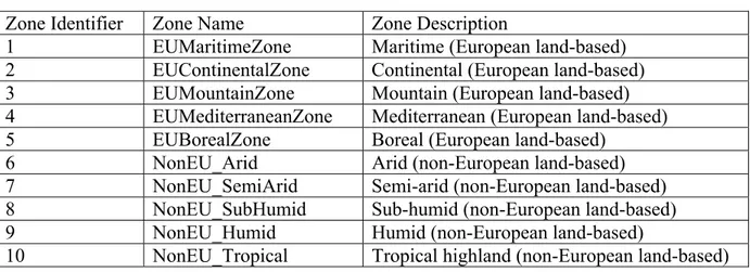
Many of the factors controlling farm-scale C and N flows are closely related to the local climate, crop types and soil types. As a consequence, most of the parameters within this model can be expected to be location-specific. The model therefore recognises a number of agroecological zones. The basic agroecological zones used in the model and for which default parameters are provided are shown in Table 1. However, users can choose to use region-specific or farm-region-specific agroecological zones, should they have location-region-specific data available. All parameters except universal constants (e.g. the universal gas constant) can be separately defined for each agroecological zone.
Table 1 Agroecological zones
Zone Identifier Zone Name Zone Description
1 EUMaritimeZone Maritime (European land-based) 2 EUContinentalZone Continental (European land-based) 3 EUMountainZone Mountain (European land-based) 4 EUMediterraneanZone Mediterranean (European land-based) 5 EUBorealZone Boreal (European land-based)
6 NonEU_Arid Arid (non-European land-based) 7 NonEU_SemiArid Semi-arid (non-European land-based) 8 NonEU_SubHumid Sub-humid (non-European land-based) 9 NonEU_Humid Humid (non-European land-based)
10 NonEU_Tropical Tropical highland (non-European land-based) The main climatic variables used in the model are the air temperature and the drought index. These are defined with monthly resolution. For air temperature, if monthly values are not available, approximate values can be calculated from the mean annual air temperature and the amplitude of the annual variation (see Appendix I).
4
3 Crop production
Provided the farm has cropped land (including pasture but excluding non-agricultural land), the farmland is considered to consist of one or more crop sequences. The number of potential crops C is a model parameter. A single crop produces Pc products, where Pc≥1. The products are defined in terms of their type and characteristics e.g. high-protein grain, low-quality straw, medium quality silage.
A submodel is used to simulate the change in C and N sequestered in the soil (see below). Since the soil submodel must simulate a number of years cropping in order to calculate the change in sequestering, the modelling of crop production must do likewise. Where more than one field/crop sequence produces the same product (e.g. spring barley grain), the production from all crop sequences/fields is pooled and averaged over the duration of the sequence in order to calculate the average annual DM production of product p from crop c (Dcrop,c,p; kg yr -1) (see Equation (0.19)).
3.1 Energy
The energy in crop production is commonly expressed in two forms. The first is the gross energy concentration of the crop product. This is the energy released if a crop product is oxidised by combustion and is mainly applied to secondary products that are utilised in this manner (e.g. straw). The second form is the concentration of energy in the crop product that is available for utilisation by livestock. There is a range of energy systems used in connection with livestock production in Europe. In principle, all energy systems designed to assess the energy in crop products that is available to livestock take the following into account:
The digestible energy of the feed. The difference between gross and digestible energy represents the loss of energy in faeces.
The metabolisable energy of the feed. This is the amount of energy available in the nutrients absorbed from the digestive system by the livestock, when the latter is working at maximum efficiency. The difference between gross and digestible energy represents the loss of energy in urine and gaseous emissions from the digestive system (principally methane).The loss of energy in urine is equivalent to about 4% of gross energy (IPCC 2006, chapter 10.3, p 10.42).
The net energy of the feed. The difference between the metabolisable and net energy represents the inefficiency with which the metabolisable energy is used for life processes (e.g. maintenance, growth). Some systems use a single efficiency factor for all life processes whereas others differentiate between the different processes.
The energy system used here is based on metabolisable energy (ME; MJ).
For each crop product, the energy available in product p of crop c (Ec,p; MJ yr-1, ME) is:
, , , ,
c p crop c p c p
E D e (0.1)
Where ec,p is the concentration of available energy in product p of crop c (MJ (kg DM)-1, ME). ec,p is a parameter.
Note: for most grain and processed crop products, the metabolisable energy concentration will be known. For roughage crop products (e.g. grass, hay, straw), the metabolisable energy concentration (MEconc,c,p: MJ (kg DM)-1, ME) can be calculated from organic matter digestibility using the relationship given on p 8 of (CSIRO, 2007):
, , 16.9 , , 1.986
conc c p OM c p
5 where ςOM,c,p is the organic matter digestibility (kg (kg organic matter)-1). The latter is given by:
, , , , , , 0.47 1 DM c p c p OM c p c p ash ash (0.2)where ashc,p is the ash content of the crop product p from crop c (kg (kg DM)-1), the factor 0.47 is the proportion of the ash that is digestible (value from Rednex project) and ςDM,c,,p is the corresponding apparent DM digestibility (kg (kg DM)-1). Both ashc,p and ςDM,c,,p are parameters.
3.2 Carbon
The annual production of carbon in crop product p of crop c (Ccrop,c,p; kg yr-1) is:
, , , , 1 ,
crop c p crop c p c p
C D ash (0.3)
where α is the C content of organic matter (kg (DM kg)-1; normally 0.46).
3.3 Nitrogen/Protein
The annual production of nitrogen (N) in each crop product Nyieldc,p (kg yr-1) is:
, , ,
c p c p c p
Nyield D n (0.4)
where nc,p is the N content of product p of crop c (kg (DM kg)-1). nc,p is a parameter.
3.4 Dry matter lost during processing and storage
Dry matter may be lost during the processing of crop products (e.g. silage making) or due to deterioration in storage. The effect of this is simulated here as follows:
, ,p , ,
pro c c p c p X X
Where Xc,p represents the C or N harvested in product p of crop c (Ccrop,c,p or Nc,p kg), ϕc,p is the proportion of the harvested material lost and Xpro,c,p is the mass lost (kg).
4 Ruminants (cattle and sheep)
Livestock are described in terms of categories of animals with specific characteristics e.g. dairy cows, heifers, bull calves. All livestock numbers are expressed as the annual average number present, not the number produced. The annual average number present is input by the user. Note that if data are only available for a number produced, this number must be multiplied by the production period expressed in years in order to obtain the average number present. For example, if the data that are available describe the number of animals produced within a category called 'Calves, birth to 6 months old', the average number of animals present will be one half of the number of animals produced.
Ruminant diets are defined in terms of feed items. A feed item can be a crop product (home-grown or imported) or it can be an imported feed or feed additive. The types of feed items in the diet and their amount are model inputs. The potential number of feed items is F, which is
a model parameter. Since all crop products are assumed to be potential feed items, F has a
6 The livestock diets are inputs to the model. It is assumed that the livestock are capable of consuming the diet fed; the model has no mechanism for constraining feed intake according to feed quality. The animal liveweight changes and milk production (if relevant) are simulated by modelling energy and protein partitioning, using a factorial approach. Energy and protein available from the diet are thus partitioned first to maintenance, then to liveweight gain and finally, if relevant, to milk production.
4.1 Intake
The annual DM intake of ruminant category g (Ig; kg yr-1) is:
, 1 F g g g f f I dZ I
(0.5)where d is the average number of days in a year (365.25), Zg is the average number of animals in category g and Ig,f is average daily DM intake of feed item f (kg) by animals in category g. Zg and Ig,f are model inputs.
The total amount of available energy available to livestock from a particular category depends partly on the composition of the diet (in particular the amount of fibre) and partly on the time during which degradation by microorganisms can occur i.e. the residence time of the feed in the rumen. The methods used to assess the energy availability in feed items normally return a value appropriate for a long residence time. For livestock with a high intake rate relative to their body size e.g. high-yielding dairy cattle, the availability of the energy in the diet will be lower than that indicated by the standard measurement methods. The variable µg is introduced here to account for this effect, where µg≤1.
The annual consumption of potentially-available energy by category g (Epot,g; MJ yr-1, ME)
is:
, , 1 F pot g g g f f f E dZ I e
(0.5)where ef is the available energy content of feed item f (MJ (kg DM)-1, ME) and a parameter. The annual consumption of available energy by category g (Eint,g; MJ yr-1, ME) is:
int,g g pot g,
E E
(0.5)
Where µg is a variable that reduces the availability of energy at high intake rate. The value of µg is dependent on the energy intake relative to the maintenance requirement (EDb,g; MJ yr-1, ME) (see Equation(0.7) ):
If Eint,g ≤ EDb,g, µg=1, otherwise
, ,
1
g b EDp g EDb g
(0.6)
where EDb,g is the energy intake above which energy availability is reduced (MJ yr-1) and µb is a parameter.
The annual intake of N by category g (Nint,g; kg yr-1) is:
int, , 0 F g g g f f f N dZ I n
(0.6)7
4.2 Maintenance
4.2.1 Energy
The maintenance energy demand of livestock category g (Em,g; MJ yr-1) is here simulated by a reduced form of the relationship used in (CSIRO, 2007):
0.75
0.03 m, int, int, 0.28 0.02 0.5 g age g g g g g dZ L e E E D (0.7)where Lg is the liveweight of the animal, ageg is the age of the animal (years) daily maintenance energy demand. If there is insufficient energy to satisfy the maintenance demand, energy is taken from body reserves (see below).
4.2.2 Protein
Protein is equated to N * 6.25. The intake of protein can therefore be defined in Equation (0.6). Part of the protein consumed is partitioned to faecal N, using the relationship provided by INRA, where faecal N (Nfaeces,g; kg yr-1) is calculated as follows:
, 6.3 0.17 int, 31.0
faeces g g g g
N dZ I N (0.8)
The remaining N (Nmet,g; kg yr-1) is available for maintenance or production:
, int, ,
met g g faeces g
N N N (0.9)
If Nmet,g is less than zero, protein is taken from body reserves (see below). 4.2.3 Remobilisation
If there is insufficient energy in the diet to support maintenance, energy is remobilised from body reserves. In this situation, an amount of energy (Eremob,g; MJ yr-1, ME) is recovered with 80% efficiency and a weight loss (Lwl,g; kg yr-1) is recorded:
, , , 0.8 remob g wl g Dpgrowth g E L e (0.10)
Where eDpgrowth,g is the concentration of energy in liveweight (MJ kg-1, ME). An associated amount of N is remobilised (Nremob,g; kg yr-1), the amount being defined as:
, , ,
remob g wl g growth g
N L n (0.11)
Where ngrowth,g is the concentration of N in liveweight (kg kg-1). Nremob,g is added to Nmet,g. If there is insufficient protein for maintenance (Nmet,g<0), N is remobilised from body reserves. The associated loss of liveweight and the energy remobilisation are calculated using equations (0.10) and (0.11), replacing energy with the appropriate nitrogenous equivalents.
8
4.3 Growth and milk production
Some or all of the energy and protein remaining after satisfying the maintenance requirements is potentially available for production. The energy available for production (Epotprod,g; MJ yr-1) is:
, int, m,
potprod g g g E E E
While the protein available is Nmet.
4.3.1 Meat-producing animals
For meat-producing animals, all the energy and protein remaining after satisfying the maintenance requirements is potentially available for growth. The growth rate is determined by whichever of the two nutrients is most limiting. The energy-limited growth rate (JEgrowth,g; kg day-1) is: , potprod, E , , growth g g growth g g growth g k E J dZ e
Where egrowth,g is the energy concentration in weight gain (MJ (kg produced)-1) and kgrowth,g is the efficiency of use of energy for weight gain. The value of kgrowth,g is calculated using the relationship taken from (CSIRO, 2007):
int, , 0.042 0.006 g growth g g E k I
The protein-limited growth rate (JPgrowth,g; kg day-1) is:
met, , , 0.7 g Pgrowth g g growth g N J dZ n
Where ngrowth,g is the nitrogen concentration in weight gain (kgN (kg produced)-1) and 0.70 is the efficiency of use of energy for weight gain.
The actual growth (Jgrowth,g; kg day-1) is then min(JPgrowth,g, JEgrowth,g). Any excess energy is assumed to be lost as heat whereas any excess Nmet is lost as urine N.
4.3.2 Dairy animals
For dairy animals, energy and protein may be used for both growth and milk production. Furthermore, some lactating livestock may support a higher milk production and can be supported from current intake, by remobilizing body tissue. These effects are simulated in the model by introducing an obligatory growth rate (Joblig,g; kg day-1) which can be either positive or negative.
9 If Joblig,g<0:
, int, m, 0.8 , , potprod g g g g oblig g growth g
E E E dZ J e
, int, , 0.7 , ,
met g g faeces g g oblig g growth g
N N N dZ J n else , , , int, m, , g oblig g growth g potprod g g g growth g dZ J e E E E k , , , int, , 0.7 g oblig g growth g met g g faeces g dZ J n N N N
As for growth, the milk production is determined by whether energy or protein is most limiting. The energy-limited milk production rate (JEmilk,g; kg day-1) is:
milk, potprod, Emilk, milk, g g g g g k E J dZ e
Where emilk,g is the energy concentration in milk (MJ (kg produced)-1) and kmilk,g is the efficiency of use of energy for weight gain. The value of emilk,g (MJ kg-1) is calculated by multiplying a unit mass of Energy-Corrected Milk (ECM)with an energy density of 3.054 MJ (kg ECM)-1; (CSIRO, 2007). The value of kmilk,g is calculated using the relationship taken from (CSIRO, 2007): int, milk, 0.02 0.4 g g g E k I
The protein-limited milk production rate (JPmilk,g; kg day-1) is:
met, , milk, 0.7 g Pmilk g g g N J dZ n
The actual milk production rate (Jmilk,g; kg day-1) is then min(JPmilk,g, JEmilk,g). Any excess energy is assumed to be lost as heat whereas any excess Nmet is lost as urine N.
4.4 Carbon
The annual intake of C by category g (Cint,g; kg yr-1) is:
int, , 0 F g g g f f f C dZ I c
(0.11)where cf is the concentration of C in feed item f (kg (kg DM)-1) cf is a parameter.
Carbon leaves the animal in the form of animal products (principally milk and meat), in excreta and as CO2 and CH4.
10 The annual exports of C in milk and meat by category g (Cmilk,g and Cmeat,g; kg yr-1) are calculated as follows:
, ,
X g g g X g
C dZ J c (0.11)
where X is either milk or meat and cX,g is the concentration of C in X (kg kg-1). cmilk,g and cmeat,g are parameters.
A proportion of the C is lost in the form of CH4. The calculation of the annual C lost (CLiveCH4,g; kg) depends upon the emission inventory system chosen:
If a Tier 2 approach is chosen, the IPCC (2006) methodology is used (Intergovernmental Panel on Climate, 2006): , 4, int, 0.365 12 16 55.65 g m g LiveCH g g GE Y C D (0.11)
where GEg is the gross energy intake of category g and Ym,g is the methane conversion factor for livestock category g.
Otherwise:
CLiveCH4,g is calculated using the relationship from (Kirchgessner et al., 1995):
4, int, 12 ( 79CF 10 212Fat 162.5N ) 16 LiveCH g g g g g g g C D NFE (0.11)where ϕg is a constant, Ng is the annual intake of N (see below) and CFg, NFEg and Fatg are respectively the proportions of crude fibre, nitrogen-free extract and raw lipid in the diet (kg (kg DM)-1). The proportions of crude fibre, nitrogen-free extract and raw lipid in the diet are calculated as a weighted average of the constituents of the diet:
,
0 int, F g f f f g g I X X D
(0.12)where X is the proportion of crude fibre, nitrogen-free extract or raw lipid in the feed item f
(kg (kg DM)-1). The proportions of crude fibre, nitrogen-free extract or raw lipid in each feed item are parameters.
The C in excreta is contained in both faeces and urine. The C excreted annually in faeces of category g (Cfaeces,g; kg) is calculated as follows:
, int, 1 ,
faeces g g g OM g
C C (0.13)
where ςg and ashg are respectively the apparent DM digestibility and the ash content of the diet of category g (kg (kg DM)-1). ςOM,g and ashg are calculated as weighted averages of the feed items in the diet, as in Equation (0.12).
The C excreted annually in urine (Curine,g; kg yr-1) is calculated as: , 0.04 int,
urine g g
C C
(0.13)
where use of the constant 0.04 assumes that the proportion of C consumed that is excreted as urine is the same as the proportion of gross energy excreted as urine (IPCC 2006).
11 The C lost from the animals as CO2 (CLiveCO2,g; kg) is then calculated by difference:
2, int, , , 4, , ,
LiveCO g g milk g meat g CH g faeces g urine g C C C C C C C
(0.13) 4.4.1 Mitigation and adaptation measures
Nitrate in the diet. If nitrate is present in the feed ration (either as nitrate deliberately added to reduce methane emission or as nitrate naturally occurring in a feed item), a fraction (nrfg) of the methane will be abated:
3
4, g LiveCH g NO nrf C (0.13)where [NO3] is the molar concentration of nitrate in the diet, [CLiveCH4,g] is the molar concentration of methane in the absence of nitrate and ϒ is an efficiency parameter.
Fat in the diet. If using a Tier 2 approach, the effect of fat in the diet must be introduced through the value of Ym. If using a Tier 3 approach, the effect will be taken into account automatically.
Supplementary feeding. If local sources of feed are not available, supplementary (imported) feed can be used.
4.5 Nitrogen
The annual export of N in milk and meat (Nmilk,g and Nmeat,g; kg yr-1) are calculated as follows:
, ,
X g g g X g
N dZ J n (0.14)
where X is either milk or meat and nX,g is the concentration of N in X (kg kg-1). Values of nX,g are parameters.
The N excreted annually in urine (Nurine,g; kg yr-1) is calculated by difference:
, int, , , ,
urine g g milk g meat g faeces g N N N N N
(0.14)
where N in faeces (Nfaeces,g) is calculated in Equation (0.8).
5 Animal housing and manure storage
The housing type is denoted by the subscript h. A given livestock category can be housed in
zero, one or two housing types; zero means that the livestock are at pasture all year round while occasions where a livestock category uses two housing types are associated with specific functions (e.g. dairy cattle will usually spend some time in a milking parlour) or pregnancy (e.g. different housing types will often be used for lactating and non-lactating sows). A range of housing types will normally be available for a given category of livestock;
the user produce manure excreta be asso availabl Figure 3 The mo animal N via N manure instance In stora approac C is par between other e matter w partition The flow 5.1 A Concep are with in anim livestoc r chooses t ed. Often, a e). However into liquid ociated with le for a give 3 Sch odelling of housing, th NH3 emissi e storage are es, the manu age, organic ches. In con rtitioned in n two fract asily degra was very lo n the organi ws of C and Animal hou ptually, the hin that hou mal housing ck feed that the housing a housing ty r, in some and solid f h a single ho en manure t hematic of th animal hou he only flux
ion and the e considered ure is stored c N and am ntrast, the T nto two frac ions, one is adable. How ow and con ic matter in d N are follo using livestock ar using for all g is conside t is spilt or
g type. The ype will onl
types of a fractions. Th ousing type type; the use
he organisat using and m es simulate e loss of u d as separat d within the mmonium N ier 2 approa tions. Somm s assumed wever, the ntributed litt nto degradab owed separa re not consi l or part of t ered to ente spoilt in th e housing t ly produce o animal hou his means t e. A range o er chooses t tion of lives manure stora ed are the ad urine C as te sources o e animal hou N are consid ach conside mers et al ( to be slowl degradation tle to the nu ble and non-ately for ea idered part the year. Th er the lives he housing type then d one type of sing there that up to tw of manure s the relevant stock, housi age currentl ddition of C CO2. Conc of gaseous e using. dered separa ers total C w (2009) parti ly degradab n rate of th utrient dyna -degradable ch animal c of the anim he feed con tock and n is consider etermines t f manure (e. is a partial wo types of storage type t manure sto
ing and man ly only con C and N in b ceptually, an emission, ev ately for bot whereas in th itioned man ble in manu he slowly d amics. For s e fractions. category. mal housing sumed by li ot the hous ed as an in the type of .g. slurry, f l separation f manure st es will norm orage type. nure storage nsiders N an bedding, the nimal hous ven though th the Tier he Tier 3 ap nure organi ure storage degradable simplicity, g, even thou ivestock wh sing. Howe nput to the h 12 f manure farmyard n of the ore may mally be e. nd C. In e loss of sing and in some 2 and 3 pproach, c matter and the organic here we ugh they hilst it is ever, the housing.
The oth form of Figure 4 5.1.1 B The am animal housing animals , g h b where ρ is the av annual a 1) is: , bedding g D where ϑ type h, to equa consum F f g
where χ χpas,g,f is A propo amount type h i , , waste g D her inputs to f bedding. 4 Inpu Bedding an mount of bed per day, th g is in use. T s housed. H h gL ρh is the bed verage livew amount of b
, , 1 g h g h ϑg,h is the p γg is the pr ate to the pr med at pastur , , , 1 int, pas g f g f g I D
χpas,g,f is 1 if s a model in ortion of th t of dry ma is: , , waste g h h o the anima uts, outputs d feed wast dding used i he number o The rate of ere, the rate dding factor weight of th bedding DM
365 g Zg proportion o roportion of roportion of re: f f feed item f nput. he feed prov atter in this
, 1 , 1 1 F h g h g f waste Z
al housing and gaseou te in animal h of animals u f use of bed e of use of b r (kg DM (k he livestock M used for a , 5bg h of the housi f the year th f the DM in f is consum vided to live waste (Dwa
, , , , pas g f g h I are from th us emission housing dep using the ho dding depen bedding (bg, kg animal liv k category g animal categing time tha hat the anim ntake of cat med at pastur estock is w aste,g,h; kg y f I he livestock s from anim ends on the ousing and ds on the ty ,h; kg DM d veweight)-1 g (kg). Both gory g in ho at livestock mal category tegory g tha re by livesto wasted by sp r-1) for live k (urine and mal housing e amount of the duratio ype of hous -1) is: d-1) for hou ρh and LG a ousing h (Db category g y g is at pas at is obtain ock type g a pillage or sp estock categ d faeces) an g f bedding ad on of the pe sing and the
(0.14) using type h are paramet bedding,g,h; kg (0.14) g spends in sture. γg is a ned from fee
(0.14) and zero oth poilage. The gory g and (0.14) 13 nd in the dded per eriod the e type of h and LG ters. The g DM yr -housing assumed ed items herwise. e annual housing
14 where ωwaste,g,h is proportion of the feed provided to livestock category g that is wasted by spillage in housing type h. The wasted dry matter is assumed to be added to the manure
produced. 5.1.2 Carbon
The C entering annually the animal housing h from category g (Cinhouse,g,h; kg yr-1) is:
, , , 1 , , , , , ,
inhouse g h g h g faeces g urine g bedding g h waste g h
C C C C C
(0.14)
where Cbedding,g,h and Cwaste,g,h are the C added annually in bedding and wasted/spoilt feed for animal category g in housing type h. Cbedding,g,h and Cwaste,g,h are calculated as:
, , , ,
X g h X g h X C D c
(0.14)
where X represents either bedding or waste. cX is the concentration of C (kg (kg DM)-1). For bedding, this is calculated as:
, , , , 1 1 , , , 1 1 1 c c P C bedding c p c p c p c p bedding C P bedding c p c p c p D a c D
(0.14)where χbedding,c,p is 1 if product p from crop c is suitable for use as bedding and zero otherwise. If no crop products suitable for use as bedding are produced on the farm, cbedding is assigned the value for a default bedding. The crop product assigned to be the default bedding is a parameter.
The C content of feed that is wasted or spoilt (cwaste,g; kg (DM kg)-1) is:
, , 1 , , , 1 1 1 1 F pas g f f f f waste g F pas g f f f I a c I
(0.14)The urine C is assumed to be as urea or low-molecular weight compounds that are very rapidly decomposed to CO2, which is then assumed to be lost to the environment. This loss of C is thus (CCO2house,g,h; kg yr-1) is:
2 , , , 1 ,
CO house g h g h g urine g
C C
(0.14)
The C from livestock category g in housing type h annually entering manure storage
(Cinstore,g,h; kg yr-1) , , , , 2, , instore g h inhouse g h CO g h C C C (0.14) 5.2 Nitrogen
The N excreted must be partitioned between ammoniacal N and organic N; gaseous emissions only occur from the ammoniacal N. The N in urine is present in the form of urea and other low molecular weight N-containing compounds. These are assumed to decompose rapidly and results in the formation of NH4-N (TAN). The annual formation of TAN from livestock excreta is equated to the urine N (Nurine,g). The N entering animal house h from livestock category g (NTANinhouse,g,h; kg yr-1) is therefore:
15
, , , 1 , , TANinhouse g h g h g urine g h N N (0.14)The organic N inputs to animal housing are from livestock faeces, bedding and spilt/spoilt feed. The annual input of organic N into the animal house h from livestock category g
(NOrginhouse,g,h; kg yr-1) is:
, , , 1 , , , , , , , ,
Orginhouse g h g h g faeces g h bedding g h bedding waste g h waste g h
N N D n D n
(0.14)
where nbedding (kg (kg DM)-1) is the N content of the bedding and nwaste,g,h (kg (kg DM)-1) is the N content of the wasted/spoilt feed. nbedding and nwaste,g,h are calculated in the same way as the relevant C contents (see Equations (0.14) and (0.14)).
TAN is lost from the animal housing via NH3 volatilisation. The annual NH3 volatilisation from animal house h that is attributable to livestock category g (NNH3house,g,h; kg yr-1) is:
3 , , , 1 3, , , ,
NH house g h g h g NH h theta TANin g h
N EF N
(0.14)
where EFNH3house,h,theta is the annual emission factor for NH3 for animal housing type h (kg (kg TAN)-1).
When using a Tier 2 approach, is a parameter constant. If using a Tier 3 approach,
EFNH3house,h,theta is the annual emission factor if livestock were housed all year round. The emission of NH3 from a given type of livestock in a given type of animal housing will vary with ambient temperature, due to its direct effect on theconcentration of NH3 in air, relative to the concentration in the manure on ventilation rates and on the indirect effect on ventilation rate. For simplicity, only the direct effect is considered here. Using Henry’s Law, the NH3 emission factor at a given mean temperature (θ; K) is expressed as a function of a reference emission factor at the mean temperature of 293K (EFNH3house,h,ref; kg (kg TAN)-1):
H,ref
3 , , 3 , ,
H,
K K
NH house h theta NH house h ref
EF EF
(0.14) Where KH,θ can be given (from Equation 27 in Hales and Drewes, 1979) as:
10 H, 1447.7 log K = 1.69 (0.14)
KH,ref is evaluated using Equation (0.14) at the reference temperature. EFNH3house,h,ref is a parameter.
For animal housing that is used year-round for part or all of the day, θ is evaluated as the
mean annual air temperature. The assumption here is that there will be an emitting surface present at all times. Where the housing is empty for part of the year, it is assumed that the housing will be cleaned when the livestock are removed. In this case, θ is evaluated as the
mean of the period during which the housing is occupied. The proportion of the year when the housing is occupied is 1-γg. Here we assume that this is a single period, centred on a particular month of the year for each livestock category (mhousing,g; month). The method used to evaluate θ is given in Appendix I.
For bot category TANinsto N 5.2.1 M Mitigat simulat 5.3 M The ma store. T type or manure manure cattle sl cattle w cows, h groupin Wishing rate of of C an The mo product Figure 5 th the Tier y g and hou , , ore g hNTAN Mitigation m ion measure ed by modi Manure sto anure from The store or types s are e storage is d e stored and lurry, with would be co heifers and b ng) is indica g to avoid t input and ra d N are trea odel does n tion of manu 5 Inpu 2 and 3 a using type h , , Ninhouse g hN measure – l es for both fying the em orage a single an r stores can e linked to defined in t d the type o crust woul onsidered on beef calves ated here us the complex ate of remo ated as if ma not consider ure from sp uts, outputs approaches, h (NTANinstore 3 , , NH house g h N ow-emissio low-emissi mission fact nimal house either be w the housing terms of the of storage. F d be separa ne type of m . A groupin ing the subs xity necessa oval of manu anure storag r flows of pecies group and losses , the TAN e,g,h; kg yr-1) on housing, on housing tor (EF NH3h can be sto within the an g type in th e livestock s For exampl ate types of manure stor ng of livesto script sg. ary to descr nure to and f ge were a ba ash or wat p sg and stor from manu entering m ) is: acidificatio and acidifi ouse,h,theta). red in eithe nimal house he database species prod le, dairy ca f storage w rage, even i ock categor ribe the con
from manur atch operati er. For late re type s (V ure storage manure stora on ication of sl er one or tw e or externa and are inp ducing the m attle slurry, hereas farm f the manur ries within a nsequences re storage, t ion. er use in th Vsg,s; m3 yr-1) age from l (0.15) lurry in hou wo types of al to it. The put by the L manure, the no crust an myard manu re came fro a species (a of variation the transfor he field, the ) is a param 16 ivestock using are f manure e storage LE. The e type of nd dairy ure from om dairy a species ns in the rmations e annual meter.
17 5.3.1 Carbon
The non-degradable C content of faeces is assumed to equate to the crude fibre content of the diet, which is calculated in Equation (0.12). Likewise, the non-degradable C content of bedding or wasted or spoilt feed is equated to its crude fibre content (CFbedding and CFwaste,g; kg (kg DM)-1). CFbedding is calculated as a weighted average of the crop products used as bedding (i.e. in a similar way as for the diet). CFwaste,g is calculated as a weighted average of the feed items fed off pasture i.e.:
, , 1 , , , 1 1 1 F pas g f f f f waste g F pas g f f f I CF CF I
(0.15)The manure may be sent to more than one type of manure store, in which case, the C must be partitioned.
The total non-degradable C from livestock category g in housing type h entering storage
annually (COrgNDeg,g,h; kg yr-1) is:
,
, , 1 int, int, , , , , ,
OrgNDeg g h g h g g g g bedding beddingg h waste g waste g h
C D CF c CF C CF C
(0.15)
where CFint,g is the crude fibre content of the diet (kg (kg DM)-1) and is calculated as in Equation (0.12).
The total non-degradable C from species grouping sg entering storage type s annually
(COrgNDegInstore,sg,s; kg yr-1) is therefore: , , , , , , 1 1 sg G H
OrgNDegInstore sg s OrgNDeg h s OrgNDeg g h
h g
C C
(0.15)
where H is the number of animal housing types, Gsg is the total number of livestock categories in the species group sg and κOrgNDeg,h,s is the proportion of the non-degradable C partitioned to manure storage s from house h.
The C input as degradable C into the same manure storage (COrgDegInstore,sg,s; kg yr-1) constitutes the remainder of the faecal, bedding and spilt/spoilt feed C:
, , , , , , , , 1 1 sg G HOrgDegInstore sg s OrgDeg h s instore g h OrgNDeg g h
h g C C C
(0.15)where κOrgDeg,h,s is the proportion of the degradable C from housing type h that is partitioned to manure storage s, The sum of the values of κOrgDeg,h,s for all the H housing types must be unity.
C is lost from storage by the emission of CO2 and CH4, represented here by CCO2St and CCH4St (kg yr-1). The values of CCO2St,sg,s and CCH4St,sg,s used here depend upon the emission inventory system that is chosen:
For Tier 2
The emission of methane C (CCH4St,sg,s) is calculated using the IPCC methodology (Intergovernmental Panel on Climate, 2006):
18 4 , , , , , , , , , , , , , 1 0.67 sg G
CH St sg s OrgNDeg h s faeces g h OrgDeg h s urine g h o sg s sg s g d C C C B MCF
(0.15)where Bo,sg,s and MCFsg,s are respectively the maximum CH4 producing capacity and the methane conversion factor for manure produced by livestock species group sg and manure
storage s.
CCO2St,sg,s is then calculated as:
4 , , 2 , , 1 CH St sg s CO St sg s C C (0.15)where τ is the proportion of the decomposed C that is emitted as CH4. τ is a parameter. The total degradation of the C in organic matter CdegSt,sg,s (kg) is then the sum of CCO2St,sg,s and CCH4St,sg,s.
For Tier 3
A relationship based on that used by (Sommer et al., 2009) is used to describe the rate of degradation of the degradable organic matter (cdeg,s; d-1):
1 ln deg, 1, app gas s Arr E R s s c b e (0.15)
where b1,s is a parameter, Arr is the Arrhenius parameter (d-1), Eapp is the apparent activation energy (J mol-1), R
gas is the universal gas constant (J K-1 mol-1) and θs is the mean temperature of the manure store during the period of storage (K). Arr, Eapp and Rgas are parameters. Note that cdeg,s is assumed to be a function of the storage type only.
The manure storage is considered here to be a batch operation with the duration of storage equal to the average length of time the manure from species group sg remains in manure
storage s (tstore,sg,s;d). The total decomposition of organic C over this period (CdegSt,sg,s; kg yr-1) is then:
deg, , ,
deg , , , , 1 s store sg s c t St sg s OrgDegInstore sg s C C e (0.15)tstore,sg,s is calculated as the average storage time for the manure from all livestock categories in the species group, weighted by the contribution of C:
, , , , , , , , 1 1 , , , , , , , , , , 1 1 1 2 sg sg G Hg OrgDeg h s OrgDeg g h OrgNDeg h s OrgNDeg g h h g
store sg s H G
OrgDeg h s OrgDeg g h OrgNDeg h s OrgNDeg g h h g C C t C C
(0.15)The emission of CH4-C is then:
4 , , deg, ,
CH St sg s sg s C C
(0.15)
The remaining decomposed C is emitted as CO2:
2 , , 1 deg, ,
CO St sg s sg s C
C(0.15)
For both Tier 2 and 3 calculations, to comply with the requirements of the soil C model (see below), the C in manure removed from the storage for application to the soil or for export must be characterised as either fresh organic C (CmanFOM,sg,s; kg) or humic C (CmanHUM,sg,s; kg). CmanHUM,g,s is calculated as:
19
manHUM, g,ss deg, ,sg s
C C (0.16)
where ϖ is a humification coefficient (dimensionless), describing the proportion of degraded
C that is converted to humic C. ϖ is a parameter. CmanFOM,sg,s is then:
, , , , , , deg, , 1
manFOM sg s OrgDeg sg s OrgnDeg sg s sg s
C C C C
(0.17)The total C in the manure store (Cman,sg,s; kg yr-1) is then;
, , manHUM, g,s , ,
man sg s s manFOM sg s
C C C (0.17)
5.3.2 Nitrogen
The TAN entering manure storage s from species group sg (NTANinstore,sg,s; kg yr-1) is:
, , , , 3 , , , 1 1 , sg G HTAN h s TANin g h NH hous
TANinst e g h h g ore sg s N N N
(0.17)where κTAN,h,s is a parameter describing the proportion of TAN from housing type h that is partitioned to manure storage s.
The N in organic matter is assumed to be associated with the degradable fraction, so the partitioning of organic N between manure storage types is assumed to be the same as for degradable organic matter.
The organic N entering the manure storage (NOrginstore,sg,s; kg yr-1) is:
Orginstore, g,s , , , , 1 1 sg G H s OrgDeg h s Orginhouse g h h g N N
(0.17)Nitrogen is lost from manure storage in the gaseous form as NH3, N2O and N2, and as TAN and organic N in surface runoff or leaching.
Organic N For Tier 2
The mineralisation of organic N in manure is assumed to be 10%, which is the default value used in the EEA/EMEP Guidebook (European Environment, 2013).
For Tier 3
We assume here that the degradation of organic matter results in a proportion of the N being bound in stable humus-like organic compounds with a constant C:N ratio of cnHUM (a parameter). The degradable organic N from species group sg in manure storage s at the end of
the storage period (NDegOrgout,sg,s; kg yr-1) is: , deg, , , , , Orginstore, g,s org s c s store sg st DegOrgout sg s s N N e (0.17)
where Ωorg,s is the proportion of organic N lost in surface run-off or leaching from manure storage type s.
20 The cumulative organic N in runoff/leaching in degradable organic matter for species group
sg and manure storage type s (Nrunoff,sg,s; kg yr-1) is:
, deg, , ,
, , , , , , deg, 1 org s c ststore sg s org s RunoffOrg sg s Orginstore sg s org s s N N e c (0.17) The amount of humic N present at the end of the storage period for species group sg andmanure storage type s (NHUM,sg,s; kg yr-1) is as follows:
, deg , , , , ,
, , , ,
org s c tstore sg s org s store sg st
HUM sg s OrgDeg sg s HUM N C e e cn (0.17)
This formulation assumes that there is no humic N in the fresh animal excreta. The runoff of humic N (NrunoffHUM,sg,s; kg yr-1) is:
, deg
deg , , , , , , , deg 1 org s c trunoffHUM sg s DegOrg sg s HUM sg s org s HUM c N C e N c cn (0.17)
The organic N ex store for species group sg and manure storage type s (NOrgoutstore,sg,s; kg yr-1) is as follows:
, , , , , ,
Orgoutstore sg s DegOrgout sg s HUM sg s
N N N
(0.17) TAN
The TAN in manure storage is supplemented by additions from the animal housing and through the mineralisation of organic N and is depleted by the emission of NH3, N2O and N2. For Tier 2
N2O emissions are calculated as:
2 , , 2 , TANinstore sg s, , Orginstore, g,s
storeN O sg s storeN O s s
N EF N N
(0.17)
where NstoreN2O,sg,s is the annual emission of N2O-N (kg yr-1, N) for species group sg and storage type s and EFstoreN2O,s is the emission factor (kg kg-1) for manure storage type s. EFstoreN2O,sg,s is a parameter and the value is taken from Table 10.21 of (Intergovernmental Panel on Climate, 2006). This formula is close but not identical to that of the IPCC; the only difference is that here, the contribution of added bedding and waste feed is included.
Annual NH3-N emissions (NstoreNH3,sg,s; kg yr-1) are calculated as:
3, , 3, , TAN , , 0.1 Orginstore, g,s
storeNH sg s storeNH sg s instore sg s s
N EF N N
(0.17)
where EFstoreNH3,sg,s is an emission factor that varies with species group sg and manure storage type s. The value of EFstoreNH3,sg,s is taken from Table 3.7 of (European Environment, 2013). The annual emission of N2 from manure storage s (NstoreN2,sg,s; kg yr-1) is:
2, , 2 , ,
storeN sg s m storeN O sg s
N N
(0.17)
21 The runoff/leaching of TAN (NrunoffTAN,sg,g; kg yr-1) is calculated as:
, , , TANinst , , 0.1 Orginstore,g,s
runoffTAN sg g TANs ore sgs s
N N N
(0.17)
The TAN ex storage (NTANOutstore,g,s; kg yr-1) is:
2 , ,, , 2, , Orginstore, g,s3, , , ,
, , 0.1
TANOutstore sg g s st
TANi
oreN O sg s storeN sg s storeNH sg nstore sg s runoffTAN sg g s N N N N N N N For Tier 3
The derivation of the relationships describing the Tier 3 dynamics of organic N and TAN in manure storage are shown in Appendix II.
The TAN ex storage (NTANOutstore,g,s; kg yr-1) is:
deg, , , , , deg, , , , , , deg, , , , , deg, , , , , , 1 1 s org s store sg s sg ss c s OrgDeg sg s t cn sg s HUM TANOutstore sg s s sum s TAN s org ssg s s OrgDeg sg s sg s H TANi U nstor s M e sg c C cn cn N e c EF cn c C cn cn N E
, , , , deg, , , , ,sum org s store sg s
EF s t s
sum s TAN s org s
sg s e c F cn (0.17)
where cnsg,s is the C:N ratio of the degradable organic matter for species group sg and manure storage type s and EFsum (d-1) is the sum of emission factors for NH3, N2O and N2 respectively (EFstoreNH3,sg,s, EFstoreN2O,s and EFstoreN2,s; d-1).
cnsg,s is defined by: OrgDeg,sg,s , Orginstore, g,s sg s s C cn N
If liquid manure is stored, the value of EFNH3,g,s is calculated using Equation (0.14), replacing EFNH3house,h,ref with EFstoreNH3,sg,s,ref (d-1; a parameter). If solid manure is stored, the temperature of the storage may depend on the ambient temperature or, if self-heating occurs, may be determined by the storage type itself. For solid storage, EFstoreNH3,sg,s is also calculated using Equation (0.14), with the exception of storage in which self-heating is considered to be dominant, where EFstoreNH3,sg,s is equated to EFstoreNH3,sg,s,ref. The value of EFstoreN2O,sg,s is a parameter.
EFstoreN2,s is calculated as for the Tier 2 method:
2, , 2 , ,
storeN g s m storeN O sg s EF EF
(0.17)
The TAN lost via runoff/leaching or gaseous emissions (NTANlost,sg,g; kg yr-1) is:
, , , , , , , , , , , ,
TANlost sg s Orginstore sg s TANinstore g s DegOrgout sg s runoffOrg sg s TANoutstore g s
N N N N N N
(0.17) The runoff/leaching of TAN (NrunoffTAN,sg,g; kg yr-1) is then:
22 , , , , , , 3, 2 , 2, TAN s runoffTAN sg g TANlost sg s TAN s NH s N O s N s N N EF EF EF (0.17)
The gaseous emissions of N (NstoreX,sg,s; kg yr-1) are;
, , , , , , 3, 2 , 2, X s storeX sg s TANlost sg s TAN s NH s N O s N s EF N N EF EF EF (0.18) Where X is NH3, N2 or N2O. 5.3.3 Mitigation measures
The mitigation measures available for manure storage are as follows: covering storage to reduce NH3 emission.
acidification of slurry to reduce NH3 and GHG emissions.
anaerobic digestion of slurry to reduce NH3 and GHG emissions.
The effect of the covering of storage on NH3 emission is simulated via the emission factor, EFstoreNH3,sg,s. The effect of the acidification of slurry (either slurry acidified in animal housing or tank acidification) on NH3 emission is also simulated via EFstoreNH3,sg,s, whereas the way the effect on GHG emissions is simulated depends on the approach used. For the Tier 2 approach, the manure conversion factor (Ym) is modified. For the Tier 3 approach, the degradation rate parameter (b1,s) is modified.
The simulation of anaerobic digestion of slurry is here limited to monosubstrate digestion (i.e. without the use of any supplementary substrate). The capture of CH4 is simulated using a gas capture efficiency factor (gcaps), such that equation (0.15) is modified as follows:
4 , , deg, ,
CH St sg s s sg s C gcap C
6 Crop and soil
The agricultural area on the farm is divided into one to many fields, each of which has a sequence of crops. Each field occupies a given area (Aseq; ha) and is a model input. In a given crop sequence r, the period number in the crop sequence (q), the crop identifier (c), starting date (tstart,q,r; yr) and end date (tend,q,r; yr) for each period in the crop sequence are all model inputs. The length of the rth crop sequence (tseq,r; yr) is:
seq,r end Q r, r, start r,1,
t t t
(0.18)
There can be no gaps in the sequence of crops; bare soil is here considered to be a crop. It is mandatory that tseq,r is an integer i.e. the last cropping period ends a whole number of years after the start of the first cropping period. This allows the crop sequence to be repeated a number of times, if necessary. Figure 6 shows an example of a cropping sequence.
Figure 6 6.1 The DM on a ra rainfall) irrigatio farmer this me DM yie produce for both N stress The pot each cro Not all reasons litter, b device u crop se calculat , , c p r Y where ψ harveste sequenc is prim harveste ξc,p is a 6 Exa Crop produ M productio ange of fac ) whereas on, supply o can influen ans that for eld i.e. the D e two crop h. The mode s. tential harv op sequence the crop ab s for this; th e stubble th used to coll equence r d ted as:
1store c p, , ψAG,c,hv is t ed and yprod ce r (kg ha -marily to pe ed either by model para ample crop s uction on of a give ctors. Some others can of nutrients nce and to ob r each perio DM yield a products (e el then adju vestable DM e (ypot,c,p,r,q; bove-ground he DM may hat is below lect the harv during perio
1 1 r Q r q A
the proporti d,q,c,r is the D 1). ψ AG,c,hv ermit the s y cutting or ameter. ωstor sequence en crop in a factors are be control s). The appr blige the us d in which achievable i e.g. grain an usts this val M productio kg DM ha-1 d DM produ y have senes w the cuttin vested mate od q that i
, , AG c hv yp ion of abov DM produc is additiona imulation o grazing, sin re,c,p is the p a given peri e not contr lled or med roach used ser to quant a crop is gr in the absen nd straw), t lue (if neces on of each 1) is an inpu duction of a sce prior to ng height of erial. The D is available , , , , prod c p r q ve-ground D ction of pro ally made sp of the resid nce the effic proportion oiod of a par rollable by diated to a here is to f tify the effe rown, the u nce of wate the user mu ssary) to all crop produ ut to the mo crop can b o harvesting f the harves M producti e for use on DM produc oduct p of c pecific to th dues remai ciency of th of DM that i rticular crop the farmer greater or focus on tho ct of other f ser must qu er or N stres ust quantify low for the uct in each del. be harvested g and fall to ter or be D on of produ n the farm (0.19) ction of cro crop c durin he harvestin ning from he latter can is lost durin p sequence r (e.g. temp lesser exte ose factors factors. In p uantify the p ss. Where c y the potent effect of w cropping p d. There are o the soil su DM that esc uct p from c m (Yc,p,r; kg op c that ca ng period q ng method, crops that n vary consi ng the proce 23 depends perature, ent (e.g. that the practice, potential crop can ial yield water and eriod of e several urface as apes the crop c in DM) is annot be q in crop hv. This can be iderably. essing of