is an open access repository that collects the work of Arts et Métiers Institute of
Technology researchers and makes it freely available over the web where possible.
This is an author-deposited version published in: https://sam.ensam.eu Handle ID: .http://hdl.handle.net/10985/7317
To cite this version :
Karim BEDDEK, Stéphane CLENET, Olivier MOREAU, Yvonnick LE MENACH - Solution of Large Stochastic Finite Element Problems – Application to ECT-NDT - IEEE Transactions on Magnetics - Vol. 49, n°5, p.1605 - 1608 - 2013
Any correspondence concerning this service should be sent to the repository Administrator : [email protected]
Solution of Large Stochastic Finite Element Problems – Application to
ECT-NDT
K. Beddek
1,2, S. Clénet
3, O. Moreau
2and Y. Le Menach
11 L2EP, Université Lille 1, Villeneuve d’Ascq 59655, France 2
Electricité De France R&D, Clamart 92141, France 3 L2EP, Arts et Métiers ParisTech, Lille 59046, France
This paper describes an efficient bloc iterative solver for the Spectral Stochastic Finite Element Method (SSFEM). The SSFEM was widely used to quantify the effect of input data uncertainties on the outputs of finite element models. The bloc iterative solver allows reducing computational cost of the SSFEM. The method is applied on an industrial Non Destructive Testing (NDT) problem. The numerical performances of the method are compared with those of the Non-Intrusive Spectral Projection (NISP).
Index Terms—Finite Element Method, Stochastic Model, Quasi Static Fields, Iterative Solver, Uncertainty Quantification.
I. INTRODUCTION
ccounting for inherent uncertainties of numerical model parameters emerges nowadays as an important step to perform robust analysis and reliability assessment. In order to quantify the effect of input data uncertainties on the quantities of interest, numerous techniques were developed. The most popular method is the Monte Carlo Simulation (MCS) method. Nevertheless, as the MCS method requires a large number of deterministic simulations to achieve high accuracy, it becomes unfeasible for very costly numerical simulations. The past decade has seen the rapid development of probabilistic spectral approaches that are based on polynomial chaos representation. The polynomial chaos expansion (PCE) methods have the advantage to exhibit a functional expression of the random quantity of interest. The Galerkin method (spectral stochastic finite element method (SSFEM)) can be applied to solve the stochastic Maxwell equations [1]. Taking advantage of the Kronecker structure of the linear systems, the storage requirement can be significantly reduced but the computation time of the solution of the linear system is still very high [2]. The non intrusive approaches like the Non Intrusive Spectral Projection (NISP) method are often preferred to SSFEM because they are easier to implement [3]. Moreover, even though the linear systems to solve are numerous, they are smaller yielding to a natural parallelization. However, the convergence proof and the error bounds are not so well established as with the SSFEM. In [9], an iterative bloc solver taking advantage of the Kronecker form of the matrix is presented. It enables the reduction of the SSFEM memory requirements. In this paper, we proposed some improvements of the iterative solver. It will be applied to solve a non destructive testing (NDT) problem. The computational costs and results obtained with the SSFEM will be compared to those given by the adaptive NISP presented in [3].
II. SPECTRAL STOCHASTIC FINITE ELEMENT METHOD
Consider a conducting domain D with a boundary Γ subdivided into M disjoint subdomains Di on which the permeability and conductivity are supposed to be random but constant and equal to µi(θ) and σi(θ) respectively (θ the outcome belonging to the event space Θ). We suppose that
the permeability µ(x,θ) (x denotes the spatial coordinates) and the conductivity σ(x,θ) on D can be written:
κ
( )
θ =∑
κ( ) ( )
θ κ≡{ }
µ σ = , , , 1 M i D i I x x i (1)with IDi(x) a function equal to 1 on Di and 0 elsewhere. The magnetic field H(x,θ), the magnetic flux density B(x,θ), the eddy current density J(x,θ) and the electric field E(x,θ) are then random fields. In the frequency domain, these fields verify the following equations:
) , x ( j ) , x ( curl ) x ( ) , x ( ) , x ( θ ω − = θ + θ = θ B E J J curlH 0 (2)
where ω is the angular velocity and J0(x) a deterministic
source term. Boundary conditions are added to (2) to insure uniqueness of the solution. As the differential operators (curl, div, grad) operate only on the spatial dimension x, potentials can be introduced, as in the deterministic case, to express the electric and magnetic fields. We consider in this paper the electric potential formulation where the stochastic magnetic potentials A(x,θ) and the stochastic electric scalar potential
φ(x,θ) are introduced such that the stochastic magneto-harmonic problem (2) reads:
(
)
(
j (x, ) (x, ))
(x) ) , x ( ) , x ( ) , x ( 0 J grad A curlA curl = θ ϕ + θ ω θ σ + θ θ µ−1 (3) We define the functional space Hcurl(D) and Hgrad(D) such that:{
}
{
0}
0 2 2 2 2 = ∈ ∈ = = × ∈ ∈ = Γ Γ E E v ), D ( v / ) D ( L v H ), D ( / ) D ( H grad curl L grad n v L curlv L v (4) We denote by L2(Θ) the space of random variables with finite variance. The unknown vector potential A(x,θ) and scalar potential φ(x,θ) are respectively sought in Hcurl(D)⊗L2(Θ) and in Hgrad(D)⊗L2(Θ). A weak form of (3) can be derived by applying the weighted residual for all u belonging to Hcurl(D)⊗L2(Θ):(
)
] ) , ( u ) ( J [ ] ) , ( u ) , ( grad ) , ( A ) , ( [ ] ) , ( curlu ) , ( curlA ) , ( [ 0 ⋅ θ γ = γ θ ⋅ θ ϕ + θ ω θ σ + γ θ ⋅ θ θ µ∫
∫
∫
− d x x E d x x x j x E d x x x E D D D 1 (5)A
where E[X(θ)] denotes the expectation of the random variable X(θ). To solve numerically the problem (5), a discrete form has to be determined on finite dimensional spaces which are subspaces of Hcurl(D), Hgrad(D) and L2(Θ).
A. Spatial dimension discretization
Usually, with the finite element method, the approximation functions used in computational electromagnetics are the Whitney shape functions [5]. We consider a mesh of D with n0 nodes, n1 edges, n2 facets and n3 elements. The space W0 of nodal shape functions and the space W1 of edge shape functions will be used as approximation subspaces of Hgrad(D) and Hcurl(D) respectively. In the following, the nodal and edge shape functions are respectively denoted w0 and w1.
B. Random dimension discretisation
In the present work, the stochastic dimension is discretized using the Polynomial Chaos Expansion (PCE). Wiener [6] was the first to suggest the use of the Hermite chaos to represent Gaussian processes. In [7], Xiu and al. generalize the concept to more general processes. Let consider a vector ξξξξ(θ)=(ξ1(θ),…,ξM(θ)) of M independent random variables. We denote fξi the probability density function of ξ1(θ). Any output Y of a given model, having as input the random vector ξξξξ(θ), can be written as mapping Y:ΘM→R. The quantity Y is a random variable and we have Y(θ)=Y(ξξξξ(θ)). Let consider ψj(ξi(θ)) a univariate orthogonal polynomial of order j with respect to the probability measure fξi. A multivariate polynomials Ψαααα(ξξξξ(θ)) defined as
( )
( )
(
M)
M i i with ,..., ) ( )) ( ( j ξ θ = α α ψ = θ Ψ = θ Ψ∏
= α 1 1 α ξ α α (6)are orthogonal with respect to the joined probability
measure
∏
≤ ≤ = m i i f f 1 ξ ξ That is to say:[
Ψα(θ)Ψβ(θ)]
= if α≠β E 0 (8)If Y(θ) has a finite variance, the PCE refers to the representation of the random variable Y(θ) as a linear combination of multivariate polynomials Ψαααα(θ):
∑
∈ θ Ψ = θ m N ) ( y ) ( Y α α α (9) In practice, the expansion (9) is truncated up to the polynomials of order p. If we denote ZMP the space of the M-tuples αααα which satisfy ||αααα||L1≤p, then the total number of polynomials in the PCE basis is equal to:! p ! M )! p M ( P= + (11)
Later, we denote by CPM the space of multivariate polynomials Ψαααα(θ) such that αααα∈ ZMP.
C. Discrete stochastic problem
In the following, we will consider the finite dimensional spaces W1⊗CPM and W0⊗CPM where A(x,θ) and ϕ(x,θ) will be approximated, that is to say:
∑ ∑
∑ ∑
= ∈ = ∈ θ Ψ ϕ ≈ θ ϕ θ Ψ ≈ θ 0 1 1 0 1 1 n i Z i i n i Z i i M p M p ) ( ) x ( w ) , x ( ) ( ) x ( A ) , x ( α α α α α αw A (12)Substituting (12) in the weak form (5) and applying the n1P test functions w1i(x)Ψαααα(θ) and the n0P test functions gradw0i(x)Ψαααα(θ) leads to a linear equation system:
AsU = Bs (11) The size of the square matrix As is equal to (NP)x(NP), with N=n0+n1, the vector U of the unknowns Aij and ϕij is of size NP The matrix As has the following Kronecker structure:
) ( ) ( i i M i i i P s σ σ = µ µ⊗ + ⊗ + ⊗ = Ι A
∑
S H S H A 1 0 (12)With Ip the identity matrix of size PxP, A0 is the mean matrix obtained by considering the deterministic magnetoharmonic problem taking the means of the reluctivity and of the conductivity (denoted µi−1 and σi) on each subdomain Di. The symmetric matrices Siµ and Siσ are of size PxP and correspond to the random dimension and their coefficients (Siµ)αβαβαβαβ and (Siσ)αβαβαβαβ (for all αααα and ββββ in ZMP) are defined such that: θ Ψ θ Ψ σ − θ σ = θ Ψ θ Ψ µ − θ µ = σ − − µ )] ( ) ( ) ) ( [( E ) ( )] ( ) ( ) ) ( [( E ) ( i i i i i i β α αβ β α αβ S S 1 1 (13) The matrices Hiµ and Hiσ are symmetric and of size N×N. The coefficients (Hiµ)jk are given by:
[ ]
else if 0 1 12 1 1 = ∈ γ ⋅ =∫
µ) d if(j,k) ,n ( k D j jk i i curlw curlw H (14)And the coefficients (Hiσ)jk by:
[ ]
]
]
[ ] ]
,n *n ,N]
) k , j ( if d w ) ( N , n ) k , j ( if d w w j ) ( n , ) k , j ( if d j ) ( k D j jk i k D j jk i k D j jk i i i i 1 1 1 0 2 1 0 0 2 1 1 1 1 , , 1 1 , ∈ γ ⋅ = ∈ γ ⋅ ω = ∈ γ ⋅ ω =∫
∫
∫
σ σ σ w grad H grad grad H w w H (15)We can notice that the matrix As is never stored entirely but only the 4M matrices Siµ, Siσ, Hiµ and Hiσ.
III. ITERATIVE BLOC SOLVER
One way to solve the linear system (11) is to use classical iterative solver and do particular matrix vector product. Another way is to use an iterative bloc solver. Let U0 an initial solution of the linear system (11). Based on [4], a bloc Jacobi iterative solver has been proposed in [9] to solve the linear system (11). The relationship between the solution obtained at the iterations i and i-1 can be written:
1 1 1 0 − − σ σ = µ µ = + ⊗ + ⊗ − = ⊗
∑
i s i j j M j j j i P ) ( ) ( T B U H S H S U A Ι (16)As the matrix (IP⊗A0) is bloc diagonal of size P, for each iteration i we solve P independent linear systems of size NxN. We can notice that the left hand side matrix is always the same and equal to A0. At each iteration i, we solve one linear system of size NxN with multiple and independent right hand sides:
A0X=V (17)
where the matrices X and V are of size NxP and defined by: P 1 1 1 + ∀ ≤ ≤ − = ((j )*N :j*N), j ) j (:, U X (18) P 1 1 1 + ∀ ≤ ≤ − = ((j )*N :j*N), j ) j (:, T V
The first advantage of this approach lies in a possible parallel computing. At each iteration step, the P linear system resolutions can be performed simultaneously. In our case, a BiCG solver has been used to solve (17). Moreover, since the matrix A0 is the same for all the linear systems to solve, a unique preconditionner can be applied to reduce the calculation time. The Ainv preconditioner was used whereas in [9] it was a diagonal preconditioner.The residual ri for each iteration i is given by:
(
1)
1 1 0 − = σ σ µ µ = σ σ µ µ − ⊗ + ⊗ = − ⊗ + ⊗ + ⊗ = − =∑
∑
i i M i i i i i s i M i i i i i i P s i s i ) ( U U H S H S B U H S H S U A I B U A r (19)By denoting ||X||2, the norm of the vector X, The stopping criterion is then defined by:
2 2 ) ( / s i i B r =
ε
(20)With respect to [9], to accelerate the convergence of the iterative procedure, we define a local stopping criterion εij for each column of the matrix X such that :
2 0 2 2 1 2 * i i j i i i j X X r r − =
ε
(21)With Xji the j-th column of the matrix X (also called j-th mode). This local criterion is such that the modes with high norms (contribute more to the global solution) are well computed and those with low norms, which contribute weakly to the global solution, are less constrained.
IV. APPLICATION AND RESULTS
Our industrial application concerns the detection investigation of clogging in tube support plate in steam generator of nuclear power plant, which may produce performances reduction and safety concern. The clogging detection is performed by an Eddy current NDT technique, called the SAX ratio, using differential bobbin coil signal. In Fig. 1, we give the variation of the flux ∆Φ in function of the
position of the probe in the tube. We can see that the variation of ∆Φ is not the same at the upper edge (∆Φin) and the lower edge (∆Φout). To evaluate the level of clogging, the idea consist in correlating the difference of magnitudes of ∆Φin and ∆Φout to the amount of deposit at the inlet foil (Fig. 1).
Fig. 1. Geometry of the studied system and the clogging detection principle.
From the control signal magnitude, a clogging SAX ratio indicator is usually extracted as:
in out SAX out Ratio ∆Φ ∆Φ ∆Φ − = (22)
Deterministic simulations are achieved using a finite element model with 1.789.946 spatial unknowns. In the probabilistic model, four parameters are assumed to be random uniform and independent variables: the conductivities and relative permeabilities of the magnetite (clogging product) and the support plate of steam generator tubes. Intervals of variation of the four considered random variables are given in Table 1. These intervals have been determined from expertise and measurements made on samples of magnetite. We fix the polynomial chaos order to p=4, leading to P=70 multidimensional polynomials in the random dimension. The quantities of interest are the flux difference between the two coils of the probe (50 positions of the probe inside the tube) and the Sax ratio. We carry out the simulation using the SSFEM method with the dedicated iterative bloc solver presented in section III and with the Non-Intrusive Spectral Projection (NISP) where a sparse adaptive grid is used to compute the multidimensional integrals [2].
TABLEI
INTERVALS OF VARIABILITY OF THE UNIFORM AND INDEPENDENT RANDOM VARIABLES OF THE MODEL
Relative Permeability Conductivity (S.m) Magnetite Uniform[ 1.3 ; 2.7 ] Uniform[ 45 ; 75 ] Tube Support Plate Uniform[ 60 ; 100 ] Uniform[ 17105 ; 18105 ]
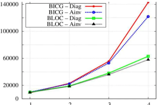
First, we compare performances of the bloc iterative solver (BLOC) to the classical BiCG iterative solver with particular matrix vector product for one position of probe inside the tube (we chose the position 16). With the BiCG solver, the whole
linear system (11) is considered during the iterative proces. In the case of the BLOC solver, at each iteration, P linear systems of size NxN are solved (see (16)). Two preconditioners are retained for the comparison: Diag for the Jacobi preconditioner and Ainv for the preconditioner based on the approximation of inverse of the matrix A0. As reported in Fig. 2, the number of matrix vector products of size N (N is equal to spatial degrees of freedom) of the bloc iterative solver increases linearly with the number of random variables (number of stochastic dimensions), whereas, this number with the BiCG increases exponentially. Notice that the Ainv preconditioner contributes slightly to the acceleration of the two solvers due to singularity and bad conditioning of the linear system resulting from A-ϕ potential formulation.
Fig. 2. Number of matrix vector product of size N (same as deterministic system) of the preconditioned BiCG and Bloc iterative solver for different numbers of random variables
In the second step, the SSFEM and the NISP methods are applied for all probe positions inside the tube. The chosen solver for the SSFEM is the bloc iterative one with global stopping criterion (20) equal to 10-9 and a local stopping criterion (21) equal to 10-6. The stopping criterion of the adaptive anisotropic procedure in the NISP has been chosen equal to 10-7 and 10-9. The computation cost of the SSFEM, reported in Fig.3, is almost the same for the whole positions of the probe. By contrast, computational costs of the NISP method are higher between the positions 10 and 25. It depends on the position probe, where the variability of the control signal is primarily located [7]. Furthermore, it can be observed that performances of the NISP are closely related to the prior stopping criterion. Both method leads to very close statistical moments on the variation of the flux. The statistical moments of the random SAX ratio obtained with the SSFEM and with a NISP (ε=10-9) are given in Table II. In that case, relative errors of 10%, 30% and 28% are obtained respectively on the standard deviation, the skewness and the kurtosis of the imaginary part of the random SAX ratio. According the size of the problem and the high sensitivity of the ratio SAX, the error between the two methods is acceptable.
V. CONCLUSION
In this paper, the SSFEM is developed in order to propagate uncertainties on the input data through an eddy current
problem. A bloc iterative method based solver is proposed to solve the resulting linear system. The SSFEM computational time and the statistical moments of the solution are compared to those given by the anisotropic adaptive NISP method. The large-scale application confirms the success of the proposed iterative solver to reduce the SSFEM computational complexity. The solver can be certainly improved by applying an efficient preconditioner to solve the multiple right hand side linear system.
Fig. 3. Number of matrix vector product of size N of the SSFEM and the NISP for each probe position. The SSFEM is equipped with bloc iterative solver (BLOC) and the NISP is equipped with adaptive anisotropic sparse grid with two stopping criteria.
TABLEII
STATISTICAL MOMENTS OF THE IMAGINARY PART OF THE SAX RATIO,
COEFFICIENT OF VARIATION AND THE NUMBER OF MATRIX-VECTOR PRODUCT OF THE SSFEM AND THE NISP
Mean S-dev. Skewness Kurtosis CV Mat-vec NISP 0.598 0.093 -0.871 2.761 15% 5.900.000 SSFEM 0.595 0.103 -1.185 3.539 17% 7.300.000
VI. REFERENCES
[1] R. Ghanem, P. Spanos. Stochastic finite elements: a spectral approach. Springer-Verlag, Berlin, 1991
[2] M. Herzog, A. Gilg, M. Paffrath, P. Rentrop and U. Wever, Intrusive
versus Non-intrusive methods for stochastic finite elements, Springer
Berlin Heidelberg, pp 161-174, 2008
[3] K. Beddek, S. Clénet, O. Moreau, V. Costan, Y. Le Menach and A. Benabou, Adaptive method for Non-Intrusive Spectral Projection -
Application on eddy current NDT, IEEE Trans. Mag.,48(2), 2012, pp.
759-762.
[4] D. Cung, M. Gutierrez, L. Graham-Brady, F. Lingen. Efficient numerical
strategies for spectral stochastic finite element models. Int. J. Numer.
Meth. Engng. 64 (2005), pp. 1334–1349.
[5] A. Bossavit: "Whitney forms: a class of finite elements for three-dimensional computations in electromagnetism", IEE Proc., 135, Pt. A, 8 (1988), pp. 493-500.
[6] N. Wiener, The Homogeneous Chaos, American Journal of Mathematics 60:897-936, 1938.
[7] D. Xiu and G. Karniadakis, The Wiener-Askey polynomial chaos for stochastic differential equations, SIAM J.Sci. Comput. 24(2), 619-644, 2002.
[8] O. Moreau, K. Beddek, S. Clenet and Y. Le Menach, Stochastic Non
Destructive Testing simulation: sensitivity analysis applied to material properties in clogging of nuclear power plant steam generators, CEFC
2012, Nov. 2012, Oita (Japan)
[9] K. Beddek, S. Clenet, O. Moreau, and Y. Le Menach, , Spectral stochastic finite element method for solving 3D stochastic eddy current problems, International Journal of Applied Electromagnetics and Mechanics, Vol. 39, Issue 1-4, 2012, pp 753-760