HAL Id: hal-01144143
https://hal-imt.archives-ouvertes.fr/hal-01144143
Submitted on 30 Jun 2015
HAL is a multi-disciplinary open access
archive for the deposit and dissemination of
sci-entific research documents, whether they are
pub-lished or not. The documents may come from
teaching and research institutions in France or
abroad, or from public or private research centers.
L’archive ouverte pluridisciplinaire HAL, est
destinée au dépôt et à la diffusion de documents
scientifiques de niveau recherche, publiés ou non,
émanant des établissements d’enseignement et de
recherche français ou étrangers, des laboratoires
publics ou privés.
Impact of Mobility on QoS in Heterogeneous Wireless
Networks
Mikaël Touati, Jean-Marc Kélif, Marceau Coupechoux
To cite this version:
Mikaël Touati, Jean-Marc Kélif, Marceau Coupechoux. Impact of Mobility on QoS in Heterogeneous
Wireless Networks. IEEE International Conference on Communications, International Workshop on
Small Cell and 5G Networks (ICC Workshops), Jun 2015, London, United Kingdom. pp.1-6.
�hal-01144143�
Wireless Networks
Mikael Touati, Jean-Marc Kelif
Orange Labs, Issy-Les-Moulineaux, France, {mikael.touati, jeanmarc.kelif}@orange.com
Marceau Coupechoux
Telecom ParisTech and CNRS LTCI, Paris, France, marceau.coupechoux@telecom-paristech.fr
Abstract—This paper develops a model evaluating the impact of mobility in heterogeneous wireless networks by the way of analytical expressions of the spatio-temporal evolution of QoS indicators. Such formulas are obtained by introducing a multi-user averaged mobility pattern named density of multi-users. Among the set of densities, we use a Gaussian form of this quantity, which results from a modeling method based on the maximum entropy principle. Numerical results show the temporal variations of the QoS indicators and highlight the combined effects of network heterogeneity due to the presence of macro and small cells, and traffic variations due to mobility.
Index Terms—heterogeneous networks, small cells, mobility, performance, quality of service, load and capacity analysis
I. INTRODUCTION
The recent and massive commercial release of wireless network connected advanced terminals and associated applica-tions has changed users way of consuming network services. Customers did not only increase their data traffic and modify their usage, but have also increased their expectations in terms of Quality of Service (QoS) in mobility. This has led Mobile Network Operators (MNOs) to define new network planning strategies, such as the deployment of heterogeneous wireless networks. MNOs evaluate network performance by the way of QoS indicators (such as load, capacity, blocking probability), which can be derived using for example the processor sharing queue assumption with or without admission control [2]. These indicators are commonly derived in static configurations (fixed base stations and users) and temporal variations are usually introduced by the way of a user redistribution in the network following probabilistic or deterministic mobility patterns.
Authors of [4][5] analyzed the LTE wireless network het-erogeneity and proposed a model evaluating the impact on coverage and throughput, showing that QoS criteria can be satisfied with reduced emitted power by the way of a spatial redeployment of stations or densification. The effect of mo-bility on α-fair scheduling policies is evaluated in [3]. In [7], authors assess the problem of mobility in a micro-cell network, each cell being divided in pico-cells. User traffic demands and mobility are defined by a triplet of the form (location of arrival, size file requirement, user velocity), each component being probabilistically distributed. They obtain expressions for some characteristic times, optimal cell sizes and maximum velocities satisfying criteria leading to a successful communication. Au-thors of [9] model mobility in an heterogeneous network (WiFi and HSDPA cells) using migration rates following Markov
Modulated Poisson Process. Using the optimal policy of the association problem, authors show that mobility improves performance under certain assumptions.
One should also mention the huge work on mobility mod-eling in the literature around ad hoc networks. To have an overview of the field one can refer to the survey by Camp and al. [14] on the mobility models commonly used in simulations of ad-hoc networks. They mainly distinguish two kinds of models, the first type being entity mobility models such as random walk, random way point, Gauss-Markov or city section models and the second one being group mobility models such as exponential correlated, nomadic community or pursue mobility models. Authors of [13] evaluate the optimal placement and the optimal number of nodes in massively dense ad-hoc mobile sensor networks. This assumption leading them to describe the nodes distribution with spatial densities.
In this paper, we jointly consider mobility, network het-erogeneity and user traffic, and we introduce a multiple-user mobility pattern based on a dynamic Gaussian user density. Such a quantity allows us to use a deterministic expression of the user spatial distribution with underlying probabilistic mobility patterns. We develop an analytical model leading to simple formulas of the spatio-temporal evolution of QoS indicators. By the way of numerical evaluations, we highlight the impact in time and space of both mobility and network heterogeneity on performance.
Section II introduces the system model, particularly the heterogeneous network model (II-A) in terms of its sub-networks, the mobility model (II-B) consisting in a Gaussian density based mobility pattern and the propagation model (II-C) leading to a simple Signal to Noise plus Interference Ratio (SINR) form (II-D). Section III defines the cell-type dependent indicators (loads, maximum throughputs, capacity) formulas. Section IV presents numerical results and gives an interpretation (IV-B) of the temporal evolution of the QoS indicators. Section V concludes the paper.
II. SYSTEMMODEL
A. Network Model
We consider a finite set M of omni-directional macro-cell base stations (MBSs) deployed on a hexagonal network made of several rings surrounding a central cell (see figure 1). Let Rc
be the half-distance between two neighboring MBSs, ρm the
2
Fig. 1. Heterogeneous network obtained by the superposition of a macro-cell base stations network and a small-cell base stations network.
macro-cell, n small-cell base stations (SBSs) are deployed with a regular pattern. Let N be the set of all SBSs of the network. Let Rn be the average half-distance between two
neighboring SBSs1, ρ
n the SBS density and Pn their common
transmit power. The superposition of the MBSs and SBSs networks results in an heterogeneous network. The coverage area of each BS is defined as the set of locations, where users are served by this station. An heterogeneous cell is made of one MBS and all the SBSs deployed in its hexagon. We define the coverage area of an heterogeneous cell as the set of locations, where users are served by the MBS or any of the SBS of the concerned heterogeneous cell. We focus our analysis on the downlink.
B. Mobility Model
In any real system, the user spatial distribution at a given in-stant can be seen as the realization of a random point process. The temporal evolution of this distribution follows however hardly identifiable mobility patterns. The group behavior of these users may be such that, in average, the number of users per unit surface is given by a density npr, tq (users{m2). Such a quantity is commonly used in physics, where systems may be described at microscopic scale (atoms, molecules) or at a larger scale while considering fluid particles whose properties result from the statistical averaging of microscopic behaviors. In this paper, we focus on this larger scale and thus do not specify any individual mobility scheme, such as random way point, random-walk or Gauss-Markov model. In other words, we consider a quantity resulting from individual mobility patterns but at a larger scale than the user point process. With this approach, we can use deterministic formulas resulting from underlying probabilistic processes. Depending on the scenarios, many forms of densities may be used.
In this paper, we will concentrate on a Gaussian density of users. With this model, the user density npr, tq has the following form:
npr, tq “ A expp´pr ´ µptqq
2
2σ2 q, (1)
where r “ pr, θq is a position vector in polar coordinates, A and σ are constants and µptq is a function of time.
A mathematical argument for this choice is provided in Appendix. It uses the maximum entropy principle that allows
1In the sense of Voronoi cells.
Fig. 2. Spatio-temporal diffusion of the Gaussian density of users in the plane. Left is at t=0s and right at t=300s.
to derive the user distribution that maximizes uncertainty, when only the mean and the variance of the radial mobility pattern are known. In addition, it is interesting to focus on such a Gaussian density due to its symmetry property and the convenience it induces in terms of interpretations. Another qualitative argument in favor of this kind of density can be provided by the way of the following example. When going out of a subway entrance, users diffuse in the plane. It seems reasonable to consider in this case an average pedestrian speed of diffusion and an isotropic radial diffusion.
To give more intuition on the model, we consider here a kind of user ”wave” spreading isotropically in a given area (figure 2). In such a case, the density goes through the cell at a velocity given by the temporal evolution of its mean µptq. The spatial extension of the distribution of users is given by the parameter σ. The total amount of users in a given area is obtained by spatial integration of the density. The previously mentioned symmetric diffusion in every angular direction of the plane allows us to locate those users of the distribution who generate a non-negligible proportion of the load. Most of the users concentrate around the mean (roughly in the interval rµ ´ 3σ; µ ` 3σs) and the spatial extension allows to catch the spreading trend. The slowest users locate at the back of the wave and the fastest ones locate at the front of the wave. Both cases are however less probable than the heights of the wave.
C. Propagation Model
We assume that the path-gain gjpuq between a station j
transmitting at power Pj and a user u only depends on the
distance rjpuq between j and u. The power, Pj,u, received by
a mobile u from j can be written: Pj,u“ PjKjr
´ηj
j puq (2)
where Kj and ηj denote the path-loss propagation coefficients
of station j. We assume constant coefficients for all stations of the same type2: K
j “ Km, ηj “ ηm @j P M and Kj“ Kn,
ηj “ ηn @j P N .
Let define Cprq as the peak data rate practically obtained in r in the absence of any other user in the cell [2]. The analytical
2For the sake of simplicity and because we focus on the mobility effect,
we ignore in this paper shadowing. We will take it into account in a future work.
by simulations of the LTE RF chain and consists in a simple fitting of obtained curves by a modified Shannon’s formula [1] of the form:
Cprq “ aW log2p1 ` bγprqq (3)
where a “ 0.6, b “ 1 and γprq is the Signal to Interference plus Noise Ratio (SINR) in r. The dependency of the system performance on the environment and on user mobility is taken into account by their impact on the SINR, which is detailed in the next section.
D. SINR
We assume that every user u is attached to its best server, i.e., the station providing the highest received signal power, u is thus served by j if and only if3:
Pjgjpuq ě Pigipuq @i P M Y N . (4)
Let now define k˚
u P M and l˚uP N the closest MBS and SBS
respectively to u. We can rewrite the previous association rule as follows. BS j is serving u is given by:
j “ k˚ if Pk˚gk˚puq ě Pl˚gl˚puq, (5)
j “ l˚ if P
k˚gk˚puq ď Pl˚gl˚puq, (6)
where we have removed the u subscript in k˚
u and l˚u for a
reason of simplicity. Finally, we can write the worst-case SINR (all stations interfering except the serving station) as:
γpuq “PmKmr ´ηm k˚ 1tj“k˚u` PnKnrl´η˚n1tj“l˚u INpuq ` IMpuq ` Nth (7) where: INpuq “ ÿ lPN ztl˚u KnPnr´ηl n` PnKnrl´η˚n1tj“k˚u (8) IMpuq “ ÿ kPMztk˚u KmPmr´ηk m` PmKmr´ηk˚m1tj“l˚u, (9) and Nthis the thermal noise power. In numerical
implementa-tions presented in section IV use the fluid model [6] to simplify the calculations of (8) and (9). We now derive in the next section the QoS indicators of the heterogeneous network.
III. PERFORMANCES
Let dSprq be an elementary surface located at r “ pr, θq. The total number of users in dSprq at t is given by:
npdSprq, tq “ npr, tq ˆ dS (10) We assume that the traffic demand is independently and identically distributed (i.i.d) among users and arrives as a Poison process of intensity λu. Flows sizes are i.i.d and given
by the random variable σf. We define the traffic density as
the average number of bits per unit of time and surface: ρpr, tq “ npr, tqλuErσfs bits{s{m2 (11)
3Indetermination is solved at random.
at t is given by:
dρdSpr, tq “ npdSprq, tqλuErσfs bits{s (12)
A. Cell load
Based on [2], we define the total load generated by a domain Dr“ Dθˆ DR served by a unique station:
ρDrptq “ ż DθˆDR dρdSpr, tq Cprq “ λuErσfs ż Dθ ż DR npr, tq Cprq dr (13) Introducing (3) in (13), we obtain a general formula giving the instantaneous load of a bi-dimensional domain Drwith users
density npr, tq: ρDrptq “ λuErσfs aW ż Dθ ż DR npr, tq log2p1 ` bγprqq dr (14)
We now detail this load formula (14) for SBSs and MBSs. 1) Small-cell load: Let Dl“ Dθlˆ DRl be the coverage
area of SBSl. In a polar coordinate system centered on SBSl,
we define the angular and radial domain such that:
Dθl“ r0; 2πs DRlpθq “ rRN0; rmaxpθqs, (15)
where RN0 denotes the minimal distance between users and
a SBS (red circles in figure 1). The extremum rmaxpθq of the
radial domain is the solution of (6), i.e., the maximum distance such that in the angular direction θ, the power received by any user from SBSl is greater than the power received from MBS
k˚. Assuming equality of the path-loss coefficients (η
m “
ηn “ η), we obtain a simple analytical expression of rmaxpθq:
rmax,lpθq “ rk˚lrcospθ ´ θk˚lq ´ a cos2pθ ´ θ k˚lq ´ As A (16) with A “ p1 ´ pPnKn PmKmq ´η{2q and pr k˚l, θk˚lq the coordinates
of MBS k˚ in the polar coordinate system centered on SBS l.
We can thus write the load generated by users in the coverage area of SBSl: ρlptq “λuErσfs aW ż2π θ“0 żrmax,lpθq r“RN0 npr, tq log2p1 ` bγprqq rdrdθ (17) 2) Macro-cell load: We now focus on the load ρkptq generated by the area covered by a macro-cell base station MBS k. To simplify its calculation, we subtract from the total load ρmk generated by the hexagon cell, the load ρml associated to the area covered by every SBS of the heterogeneous cell. We thus obtain the following formula:
ρkptq “ ρmk ptq ´ n´1 ÿ l“0 ρml ptq (18) The load ρm
k involves a numerical integration over a convex set
(the hexagon), while loads ρm
l involve numerical integrations
similar to (17), i.e., over convex sets. The serving area of a MBS is a priori non-convex. On the contrary, the right hand side of (18) involves only numerical integrations over convex areas, which makes easier the load computation.
4
B. Cell capacity
Capacity may admit many definitions. We consider the one given in [2]. It is defined as the maximum average value of total traffic in bits/s (reached at the limit of overload, i.e., when load tends to 1). We have previously defined the demand of an area as the one resulting from the activity of users distributed according to a spatial density. Thus, we first define the maximum throughput per user of a MBS or a SBS as the maximum average value of individual traffic (bits/s/user) knowing that the service is uniformly distributed among all users. In case of heterogeneous cells, we define the capacity as the maximum total average traffic (bits/s), still knowing that the service is uniformly distributed among all users.
1) Small-cell maximum throughput: The maximum throughput per user served by SBSl is given by:
Qpl, tq “ sup ρlă1 λuErσfs “ aW ˜ ż2π θ“0 żrmax,lpθq r“RN0 npr, tq log2p1 ` bγprqq rdrdθ ¸´1 (19) 2) Macro-cell maximum throughput: The maximum throughput per user served by MBS k is given by:
Qpk, tq “ sup ρkă1 λuErσfs “ aW ˆ ż2π θ“0 żRe r“RM0 npr, tq log2p1 ` bγprqq rdrdθ ´ n´1 ÿ l“0 ż2π θ“0 żrmax,lpθq RN0 npr, tq log2p1 ` bγprqq rdrdθ ˙´1 (20) with RM0 the minimal distance between users and any MBS
and Re the radius of the disk equivalent in surface to the
hexagonal coverage of the macro-cell.
3) Heterogeneous-cell capacity: Finally, we define the ca-pacity of an heterogeneous macro-cell as the total number of bits per unit of time that the system is able to transmit to users it is serving. This quantity is obtained by adding all individual maximum throughput: Chpk, tq “ nkptq ˆ Qpk, tq ` n´1 ÿ l“0 nlptq ˆ Qpl, tq (21)
where nkptq denotes the total number of users served by MBS
k, nlptq denotes the total number of users served by SBS l
(lth small-cell station contained in the hexagon of MBS k). Equations (17), (18), (19), (20) and (21) allow us to quickly compute the loads and capacities in a heterogeneous network.
IV. SCENARIO ANDRESULTS
In this section we present the numerical results obtained from the previous analytical approach. Our aim is to show the impact of mobility (due to the spatio-temporal evolution of the density of users) on QoS indicators such as loads or capacity.
−2000 −1500 −1000 −500 0 500 1000 1500 2000 −1500 −1000 −500 0 500 1000 1500
Fig. 3. Network of heterogeneous cells. Macro-stations are identified by the symbol d, small-cell stations by `. The first ring around each ` gives the minimal distance to small-cells. Each small-cell coverage area (given by equation (16)) is in dotted lines.
A. Assumptions
We consider a scenario with two SBSs per heterogeneous cell. The half distance Rc between two MBSs is 866 m and
the distance Rr between any SBS and the MBS at the center
of its heterogeneous cell is 500 m. The minimum distance RM0 to a MBS is 50 m and the minimum distance RN0 to
a SBS is 30 m. The MBS transmitting power Pm is 43 dBm
and the SBS transmitting power Pn is 28 dBm. The path-loss
parameter η is 3.41. The signal bandwidth W “ 10 MHz. There are Ntot“ 30 users initially introduced in every
macro-cell and their individual average traffic intensity λuErσfs is
100 kbits/s.
The network layout is shown on figure 3. All hexagon cells are identical in terms of SBS deployment, we thus focus on the central cell for numerical experimentations.
We propose a Gaussian density of users with mean µptq “ RM0` 3σ ` vt, normalized at any instant to Ntot. The density
goes through the cell in time at velocity v “ 1 m{s (average speed of a pedestrian). Changing the average pedestrian speed v would only induce changes in the time-scales of the temporal variations of the indicators shown in this section (others such as failures if considered may behave differently). The model remains valid for any other density as long as it can be written in the form npr, tq. If the expressions in the paper are analyt-ically tractable then the temporal evolutions are obtained, if not they can be evaluated by numerical computations. B. Results and Interpretation
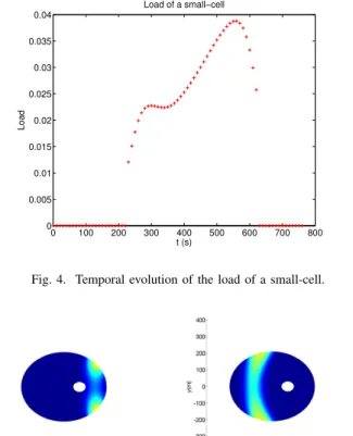
1) Load of a small-cell: Figure 4 shows the time variations of a SBS load. These variations are due to the dispersion of users in the plane via the diffusion of their density. We particularly observe a sudden jump at time t “ 230 s, which corresponds to the first arrival of a user in the small cell coverage area. Then, we can observe the user ”wave” traversing the small cell: the loads reaches a global maximum at t “ 560 s before decreasing to zeros when the last user leaves the serving area.
Interestingly, we observe a local maximum if the load around t “ 300 s. This is due to the fact that after this time
0 100 200 300 400 500 600 700 800 0 0.005 0.01 0.015 0.02 0.025 0.03 0.035 t (s) Load
Fig. 4. Temporal evolution of the load of a small-cell.
Fig. 5. Evolution of the load density in a small-cell coverage area (whithe circle is the SBS location). Left is at t=300s and right at t=520s. Dark shades indicate low values and bright shades indicate higher ones.
instant, the peak number of users served by the SBS is reached and these users start to be in average closer to the base station. They thus tend to obtain higher physical data rates and create less load on the small cell. As the maximum of the wave starts going farther from the base station, data rates decrease and the load increases again. At t “ 560 s, this effect starts to be compensated by the fact that more and more users are leaving the serving area. Figure 5 illustrates this phenomenon by showing the SBS load density at two time instants.
2) Load of a macro-cell: Recall that users diffuse from the central MBS towards the cell edge. This means that the SINR of a user going away from its initial serving MBS decreases due to the weakening of its useful signal (path-loss effect) and the growing interferences. This explains the fact that the macro-cell load is first increasing (see figure 6). At t “ 230 s, the load is a bit stabilizing (at least increases with a lower slope). At this time instant, SBSs are indeed starting serving users, alleviating some load from the MBS. From 470 s to 720 s, we observe again a high load increase. This effect being due to both users going back from small-cell to macro-cell coverage area and the global mobility towards the cell edge. At t “ 720 s, small cells do not serve any user and users start leaving the macro-cell coverage area.
3) Capacity of an heterogeneous-cell: The capacity varia-tions observed on figure 7 result from the users weighted sum (21) of the temporal evolutions of the maximum throughputs of each serving cell (20) (19). These individual variations are
0 100 200 300 400 500 600 700 800 0 0.1 0.2 0.3 0.4 0.5 0.6 t (s) Load
Fig. 6. Temporal evolution of the load of a macro-cell.
0 100 200 300 400 500 600 700 800 0 5 10 15 20 25 20 35 40 45
Capacity of an heterogeneous cell
t(s)
capacity (Mbits/s)
Fig. 7. Temporal evolution of the capacity of an heterogeneous cell.
obtained by inversion of the previously analyzed load varia-tions. The gain in the heterogeneous-cell capacity obtained as a result of the introduction of small-cells is significant. When SBSs start serving (t “ 230 s), we observe an increase of 92% in capacity, rising from 18.6 Mbits/s to 35.7 Mbits/s. Similarly, when the service of SBSs stops (t “ 620 s), the capacity of the heterogeneous cell decreases of 62% from 1.61 Mbits/s to 0.61 Mbits/s.
V. CONCLUSION
In this paper, we developed an analytical model to study the impact of mobility on QoS in heterogeneous wireless net-works. We introduced a multi-user averaged mobility pattern by the way of a quantity named ”density of users”. To illustrate this notion, we have chosen a dynamic Gaussian form. We established simple expressions of the temporal evolution of performance indicators such as load, maximum throughputs or capacity. Numerical results showed this evolution and we gave an interpretation of their variations based on the known dynamic of the Gaussian density of users. We noticed the
6
stabilization of the load of a macro-cell and the significant increase of the capacity of an heterogeneous cell, both induced by the entrance of users in the coverage area of small-cells. Future work may include other forms of user densities and take into account more complex propagation models such as shadowing and fast-fading.
APPENDIX
We propose hereafter a proof justifying the Gaussian form of the density of users we use in the proposed model. This proof includes a modeling method using the maximum entropy principle; see [10], [11], [12] and references therein. Basically, we are looking for the mobility model we are legitimately able to assume when only knowing the mean and variance of the radial mobility pattern of users.
We define r, the matrix containing at row i the two random polar coordinates pri, θiq of user i among Ntotusers and P prq
the joint probability distribution of the random components of matrix r. Let consider the following assumptions:
@i, ż dr r2iP prq “ σ2ri “ σ 2 and ż drP prq “ 1 (22) We are looking for the probability distribution of the coor-dinates of users maximizing uncertainty. Thus, we define the Lagrangian LpP q such that:
LpP q “ ´ ż drP prqlogpP prqq `ÿ i γipσ2´ ż drr2iP prqq ` βp1 ´ ż drP prqq (23) Taking the functional derivative of LpP q with respect to P :
δLpP q
δP “ 0 ô ´1 ´ logpP prqq ´ ÿ
i
γir2i ´ β “ 0 (24)
We obtain the following form for the distribution: P prq “ź i P pri, θiq (25) with: P pri, θiq “ e´pγir 2 i` β`1 Ntotq (26)
Using (22), we evaluate the Lagrange multipliers:
e´pβ`1q“ 1 p2πσ2qNtot2 πNtot and @i, γi“ 1 2σ2 (27) Finally, we have: @i, P pri, θiq “ 1 ? 2πσ2 1 πe ´r2i 2σ2 (28)
Now assuming the knowledge of the mean of each radial component Erris “ µi “ µ and its variance Erpri´µq2s “ σ2,
we obtain (using the same method) the following spatial distribution for the coordinates of user i:
@i, P pri, θiq “ 1 ? 2πσ2 1 πe ´pri´µq2 2σ2 (29)
Let define the average number of users in an elementary surface dSprq (section III) as:
N pdSprqq “ÿ
k
k ˆ P pk users in dSprqq (30) This probability of having k users (among Ntot) in dSprq
being given by the following binomial distribution: P pk users in dSprqq “ ˆ Ntot k ˙ pkp1 ´ pqNtot´k (31)
with p the probability of a user being in dSprq: p “ P pr, θq ˆ dSprq “ ? 1 2πσ2 1 πe ´pri´µq2 2σ2 ˆ dSprq (32)
Knowing the mean of a random variable following a binomial distribution, we obtain: N pdSprqq “ Ntotˆ p “ Ntot 1 ? 2πσ2 1 πe ´pr´µq2 2σ2 ˆ dSprq (33) Defining the density of users as the average number of users per unit area (users{m2), we finally have the Gaussian form
of the expected density of section II-B: nprq “ Ntot 1 ? 2πσ2 1 πexp ´pr´µq2 2σ2 (34) REFERENCES
[1] C.E.Shannon, A mathematical theory of communication, Bell Labs Tech. J., vol.27, pp.379 - 457, 1948.
[2] T. Bonald and A.Proutiere, Wireless downlink data channels: user perfor-mance and cell dimensioning, ACM MobiCom, pp.339 - 352, Sep. 2003. [3] S.C.Borst, N.Hegde, A.Proutiere, Mobility-driven scheduling in wireless
networks, IEEE INFOCOM, pp.1260 - 1268, Apr. 2009.
[4] J-M.Kelif and W.Diego and S.Senecal, Impact of transmitting power on femto cells performance and coverage in heterogeneous wireless networks, IEEE WCNC, pp.2996 - 3001, Apr. 2012.
[5] J-M.Kelif and S.Senecal and M.Coupechoux, Impact of small cells location on performance and QoS of heterogeneous cellular networks, IEEE PIMRC, pp.2033 - 2038, Sep. 2013.
[6] J-M.Kelif and M.Coupechoux and P.Godlewski, A fluid model for per-formance analysis in cellular networks, EURASIP Journal on Wireless Communications and Networking, 2010.
[7] S.Ramanath and V.Kavitha and E.Altman, Spatial queuing analysis for mobility in pico cell networks, WiOpt, May 2012.
[8] P.Barsocchi, Channel models for terrestrial wireless communications: a survey, National Research Council - ISTI Institute.
[9] P.Coucheney and E.Hyon and J-M.Kelif, Mobile association problems in heterogeneous wireless networks with mobility, IEEE PIMRC, pp.3129 -3133 Sept. 2013.
[10] M.Debbah, and R.R.Muller, MIMO channel modeling and the principle of maximum entropy, IEEE Transactions on Information Theory, vol.51, no.5, May 2005.
[11] M.Guillaud and M.Debbah and A.L.Moustakas, Maximum entropy MIMO wireless channel models, arXiv:cs/0612101, 2006.
[12] E.T.Jaynes,Information theory and statistical mechanics, The Physical Review, vol.106, pp.620 - 630, May 1957.
[13] A.Silva and E.Altman and M.Debbah and G.Alfano, Magnetworks: how mobility impacts the design of Mobile Networks, IEEE INFOCOM, Mar. 2010.
[14] T.Camp, J.Boleng, V.Davies, A Survey of mobility models for ad hoc network research, Wireless Communications and Mobile Computing, vol.2, pp.483 - 502, 2002.