Can demography affect inflation
and monetary policy?
Mikael Juselius and Előd Takáts
23 September 2014
Abstract
Several countries are concurrently experiencing historically low inflation rates and ageing populations. Is there a connection, as recently suggested by some senior central bankers? We undertake a comprehensive test of this hypothesis in a panel of 22 countries over the 1955-2010 period. We find a stable and significant correlation between demography and inflation. In particular, a larger share of young or old is correlated with higher inflation, while a larger share of working age cohorts is correlated with lower inflation. The results are robust to different country samples, time periods, control variables and estimation techniques. We also find a significant albeit unstable relationship between demography and monetary policy.
The views expressed here are those of the authors and do not necessarily represent those of the Bank for International Settlements. We are grateful for comments from Claudio Borio, Matthias Drehmann, Andrew Filardo, Enisse Kharroubi, Madhusudan Mohanty, Adrian van Rixtel, Hyun Song Shin, Philip Turner, and Fabrizio Zampolli and from seminar participants at the BIS headquarters and the Asian Office for useful comments. We thank Emese Kuruc for excellent research assistance. All remaining errors are our own.
Motivation
Why was inflation in advanced economies high in the 1960s and 1970s and why is it low today? The conventional view is that central banks made mistakes in the past which allowed inflation to slip higher and higher. Only when they started to combat inflation in the 1980s, did it moderate. However, recently some senior central bank officials have offered an intriguing alternative to this “pure mistake” view, arguing that low-frequency inflation may be linked to demographic change (Bullard et al (2013) and Shirakawa (2011a, 2011b, 2012 and 2013)). Similar arguments also appear in recent IMF working papers by Anderson et al (2014) and Imam (2013). While unconventional, such a hypothesis may deserve closer scrutiny especially in light of the deflationary pressures witnessed today in some ageing advanced economies. Hence, we should not dismiss this hypothesis offhand, but rather subject it to careful empirical testing.
In this paper, we investigate the link between demography and inflation using data from 22 advanced economies over the 1955-2010 period. We find a stable, statistically and economically significant relationship between the age structure of population and inflation. Demography accounts for around one-third of the variation in low-frequency inflation and for the bulk of the inflation deceleration between the late 1970s and early 1990s. Furthermore, our estimates reveal a stable U-shaped pattern: a larger share of young or old is correlated with higher inflation, and a larger share of working age cohorts is correlated with lower inflation. While our benchmark specification controls for real interest rates and output gaps, the results are robust to extensive changes to the specification. Varying the sample, adding controls and using increasingly sophisticated estimations techniques does not change the result. The relationship remains intact if, for instance, the time period is restricted to 1995-2010 or time fixed effects are added. In short, we find a robust empirical link between demography and inflation.
The robust correlation between demography and inflation is puzzling and raises the question of why central banks did not offset it. In order to shed some light on this question we extend our analysis to monetary policy. We also find a significant relationship between demography and monetary policy but, in contrast to inflation, this relationship is not stable over time. In the first half of the sample, before the 1980s, monetary policy reinforced the demographic impact of inflation: real interest rates were low precisely when demographic pressure was high. However, this pattern reversed in the second half of the sample: after the 1980s monetary policy started to lean against the demographic inflationary pressures.
Our findings on inflation are related to some earlier works on inflation forecasting. McMillan and Baesel (1990) used correlation between demographics and inflation in the US context to predict the moderation of inflation in the 1990s. Using data from 20 OECD countries over the 1960-1995 period, Lindh and Malmberg (2000) also found strong correlation between age structure and inflation which they used to forecast inflation rates. In line with our results, both papers report a positive inflationary impact from the young and the old and a negative impact from working age cohorts. However, our paper differs from these papers both in terms of substance and in technical aspects. In terms of substance, we do not remain content with analysing the correlation between inflation and demography but investigate the question in a broader monetary policy setting context. In terms of technical aspects, we use a larger sample and more
sophisticated estimation techniques. In particular, we use population polynomials, first developed in Fair and Dominguez (1991), to efficiently exploit the entire age structure of the population. Moreover, we allow for country heterogeneity and estimate dynamic heterogeneous panels in error correction form to avoid spurious results.
While our main contribution is to carefully document the empirical link between demography, monetary policy and inflation, we also explore potential theoretical explanations for the observed pattern. As we discussed earlier the observed empirical pattern contradicts the conventional view: demography seems to affect inflation even after controlling for real interest rates and output gaps. One potential explanation is that demography affects the equilibrium real interest rate. To formalize the argument, we derive an overlapping generation model with lifecycle that can generate – without central bank action – a similar empirical pattern of inflation and real interest rates that we see in the first half of the sample, i.e. when central banks did not offset demographic pressures on inflation.
While this model might be a useful stepping stone to understand how demographic pressure works, it cannot explain why central banks started to lean against inflationary pressures after the 1980s. Though our research was partly motivated by Bullard et al (2013), the empirical pattern that emerges from our investigation is not fully consistent with the political economy model of central banking: the non-voting young have a sizeable inflationary impact and, perhaps more importantly, the impact of different age cohorts on monetary policy is unstable. Thus, the behavior of monetary policy, and thereby that of inflation, is a puzzle – one that clearly requires a deeper theoretical understanding.
Our results suggest that demography leads to inflationary pressures which affect, at the central banks’ discretion, either inflation or real interest rates. Furthermore, the estimates suggest that the current benign environment of low inflation and low real interest rates is a product of favorable demographic trends. Demographic tailwinds lowered inflation pressures by around four percentage points from 1970 to 2010. However, this benign environment will not last. As populations in all advanced economies will age over the next forty years, the tailwinds are expected to turn to headwinds: demographic inflationary pressures are expected to rise by around four percentage points on average between 2010 and 2050. This implies that central banks might well have to raise real interest rates more aggressively than in the recent past to avoid higher inflation.
The rest of the paper is organized as follows. The next section describes the data that we use in our analysis. The third section establishes the empirical link between inflation and demography and shows that it is robust over several alternative setups. The fourth section investigates how demography affects the conduct of monetary policy. The fifth one introduces a model of demographic demand and evaluates some potential theoretical explanations. The sixth one discusses the findings from different perspectives. The seventh and final section concludes with policy implications.
Data
We include the largest possible available sample. In terms of time coverage, we use almost the full postwar sample: from 1955 to 2010. We do not use the years right after World War 2, because of the impact of the post-war reconstruction - and to a smaller extent that of the Korean war.1 In terms of countries, we cover the 22
advanced economies for which data is available in good quality: Austria, Australia, Belgium, Canada, Switzerland, Germany, Denmark, Spain, Finland, France, Greece, Ireland, Italy, Japan, Korea, the Netherlands, Norway, New Zeeland, Portugal, Sweden, United Kingdom and the United States. In short, our sample covers 22 countries over 55 years.
The main variable of interest is the yearly inflation rate obtained from Global Financial Data and national data sources. Given that we are interested in low frequency inflation dynamics yearly data is sufficient. In the following, we denote yearly inflation as , where j=1,…,N is a country index and t=1,…,T is a time index. A cursory look at the inflation data confirms the substantial variation both across time and countries (left-hand panel, Graph 1). The United States highlights a typical time trend: inflation rose in the late 1960s and started to moderate rapidly after the late 1970s peak (black line). However, there is also substantial heterogeneity across countries (red band): inflation did not always moderate in lockstep with the US and there are many idiosyncratic jumps in many countries.
Inflation and dependency ratio
In per cent Graph 1
Inflation Dependency ratio
The other main variable of interest is demographic data on the age structure of the population obtained from the UN population database. Besides historic data we will also use the median forecasts. The data divides total population (denoted as
1 Technically, observations are available from 1950 onwards. However, many economies, including
the US experienced abnormal hikes in inflation between 1950 and 1955 following the onset of the Korean War. Similarly, we exclude the years following the 2008-09 financial crisis where low growth led to low inflation in a number of countries. However, this sample choice does nor drive our results: using data from the full postwar years yields results both quantitatively and qualitatively similar to using the 1955-2010 sample with the precision of the estimates only marginally reduced.
–5 0 5 10 15 20 1960 1970 1980 1990 2000 2010 United States 20 40 60 80 100 120 1960 1970 1980 1990 2000 2010
for each country and year) into 17 five-year age cohorts (denoted by where = 1, … ,17) where the shows the number of persons in cohorts 0-4, 5-9, 10-14, 15-19, 20-24, 25-29, 30-34, 35-39, 40-44, 45-49, 50-54, 55-59, 60-64, 65-69, 70-74, 75-79, and 80+. We also denote the share of cohort k in the total population,
/ , by . Fur future use we also define the share of young population (0-19 years old population), = ∑ , the share of working population (20-64 years), = ∑ , and the share of old (65 years and older), =
∑ .
The dependency ratio, i.e. the young and old population divided by the working population ( = 100 ∗ ( + )/ ) provides a summary statistic for demographic change. As its name suggests, the dependency ratio approximately captures the share of the population which is economically dependent in the sense that they cannot earn labor income. For example, a value of 50 for this ratio implies that the working population is twice as large as the dependent population. In our dataset, the dependency ratio declined in general as the baby boomers typically had fewer children than their parents. However, there was quite a bit of heterogeneity in this decline (Graph 1, right-hand panel). Interestingly, the United States (black line) has roughly typical dependency ratios in the early part of the sample, by today it has one of the highest rate.
In addition to the inflation rate and the population variables, we use a number of control variables. Given that inflation is a monetary phenomenon, it should also be related to the real interest rate, . In most of our analysis we use the ex-post real interest rate given by = − , where is the nominal overnight interbank interest rate. To get full time coverage, we collect the nominal interest rates from several different sources: national data, Datastream, and Global Financial Data.
One disadvantage of using ex-post rate as an explanatory variable is that inflation appears on both sides of the econometric equation, albeit in constrained form on the right hand side. Aside from obvious endogeneity issues, already the two large outliers associated with the oil crises in the 1970’s, for instance, would generate high significance for this variable. For these reasons we also use one-year ahead inflation forecasts from Consensus Forecasts, , to construct an ex-ante real interest rate, = − . Unfortunately, this ex-ante real interest rate is only available after 1989 in most countries.
Furthermore, standard models would suggest that inflation is related to the output gap, = − ∗, where real GDP ∗ is potential GDP. Given the length
of the sample, we obtain real GDP figures from a variety of sources: national data, OECD Economic Outlook, IMF WEO, Datastream, and Global Financial Data. We then construct a measure for the output gap with full sample coverage, by using the deviations in real GDP from a Hodrick-Prescott filtered trend (with λ is set to 100, the standard value for yearly frequency).
We also use four additional control variables which may be particularly relevant for low-frequency inflation. We examine the growth in the ratio between the broad money stock ( 2 ) and GDP. The statistics on M2 is obtained by combining several sources: national data, the European Central Bank, OECD Economic Outlook, IMF IFS, and Global Financial Data. The time coverage of the money stock varies from country to country, but starts in all but two countries before the 1980s. We also consider the fiscal balance as a share of GDP (denoted as ( − )/ ) that we obtain from IMF WEO. The sample for the fiscal variables starts, at the earliest, in
1980, but some countries do not have any observations before 1995. Finally, we try two measures of asset price inflation; residential property price inflation, , from the BIS Residential Property Price Database, and equity price inflation, from Global Financial Data. They are generally available from 1970 onwards.
Demography and inflation
We provide a comprehensive empirical analysis of the suspected relationship between inflation and demography in this section. We begin by trying a simple univariate measure of the demographic structure, the dependency ratio, as a regressor. We find that it is significant both in statistical and economic terms. Given this finding, we gradually extend the analysis, taking the entire population structure more fully into account, and conduct a number robustness checks to see if we can make the relationship disappear. Among others, we include a number of control variables and time fixed effects, use alternative time periods and country samples, and different estimation techniques. The relationship remains intact regardless of these alterations.
First glance at the data: from graphs to population polynomials
We begin by graphically comparing a common univariate summary measure of the demographic structure – the dependency ratio – with inflation. As the ratio is often used in studies examining the impact of demographic change, it is a good starting point for our investigation.
Graph 2 shows some positive correlation between inflation (scale on left hand axis) and the dependency ratio (scale on right hand axis) for the average of our sample, and separately for five major advanced economies. Interestingly, the correlation seems to be the weakest for Japan, the country for which some policymakers and researchers see demography as a serious potential explanation for inflation. The graph also reveals that both demographic and inflationary time-patterns have been fairly similar across countries even if the magnitudes of the series have differed. This opens up the possibility that the time correlation between the two variables is purely coincidental, with inflation being driven by some common factor across countries. We will address this possibility by providing two estimates for each specification: one without time fixed effects and one with such effects included.
To get a more formal sense of the connection in Graph 2, we regress inflation on the dependency ratio:
= + + + (1)
where is the constant and is a country specific fixed effect. Given that demography is reasonably exogenous to most economic variables, large endogeneity issues should not arise in (1).
The dependency ratio appears to be strongly correlated with inflation (Table 1). Model 1 in the first column shows that the dependency ratio alone explains around 16% of the within variation of low frequency inflation. Controlling for time-fixed
effects (Model 2) leads to a slight drop in the estimated coefficient on the dependency ratio, but it nevertheless remains both economically and statistically significant. In fact, the drop should not be surprising as Model 2 mostly captures cross-country, rather than temporal variation in the data. Taken together, these two results suggest that we cannot immediately reject a relationship between inflation and demography.
Inflation and dependency ratio
In per cent Graph 2
Average United States United Kingdom
France Germany Japan
Next, we allow for slightly more flexible demographic effects. In particular, the dependency ratio implicitly assumes that the young and the old have identical effects and these effects have the opposite sign but the same absolute size as the effect of the working age cohorts. To explore the robustness of this implicit assumption we extend the estimation to allow these three age cohorts to have different effects, ie formally we estimate the below regression:
= + + + + (2)
Notice that equation (3) does not have a constant. The reason is that the three population shares sum to one, hence, they would be perfectly correlated with the constant.
Allowing for more flexibility vis-à-vis the effects of different age groupings does not alter the picture substantially. This can be seen from the Models 3 and 4 in Table 1 which report the estimates of equation (2) with and without time fixed effects, respectively. First, note that the explanatory power hardly increases compared to Models 1 and 2. The likely reason is that the implicit assumption
0 3 6 9 12 60 66 72 78 84 1970 1990 2010 Inflation (lhs) –4 0 4 8 12 60.0 67.5 75.0 82.5 90.0 1970 1990 2010 Dependency ratio (rhs) 0 5 10 15 20 67 70 73 76 79 1970 1990 2010 –5 0 5 10 15 65 70 75 80 85 1970 1990 2010 –2 0 2 4 6 55 60 65 70 75 1970 1990 2010 –6 0 6 12 18 50 60 70 80 90 1970 1990 2010
behind using the dependency ratio is roughly satisfied: the young and the old have approximately the same impact on inflation, and the working age population has the same absolute size impact with the opposite sign. Furthermore, using these population cohorts reveals that the two dependent population categories increase inflation whereas the working age cohorts decrease it – one could see a U-shaped pattern emerge. This cohort specific finding is not visible from the estimation using only the dependency ratio. Adding time effects again reduces significance levels, in particular for the old age category which now becomes statistically insignificant. However, time fixed effects do not eliminate the overall demographic impact.
Demography and inflation
Dependent variable is t Table 1
Model 1 2 3 4 5 6 depr 0.17 (11.16) (4.10) 0.11 n 0.31 (10.61) (3.42) 0.22 n –0.23 (–7.67) (–5.89) –0.14 n 0.31 (4.25) (0.11) 0.01 n (× 1) 1.95 (14.15) (0.87) 0.12 n (× 10) –4.62 (–14.97) (–3.29) –1.09 n (× 10 ) 3.90 (14.62) (4.84) 1.38 n (× 10 ) –1.07 (–13.92) (–5.93) –0.48 const. –12.28 (–11.59) (–7.12) –9.87 NA NA –202.89 (–10.78) (2.49) 46.07
Dem. Insig. F-test 0.000 0.000
Country effects Yes Yes Yes Yes Yes Yes
Time effects No Yes No Yes No Yes
R 0.16 0.57 0.16 0.57 0.30 0.61
Obs. 1276 1276 1276 1276 1276 1276
Max sample 1955-2010 1955-2010 1955-2010 1955-2010 1955-2010 1955-2010
Note: We obtain valid R2 estimates for model 3 and 4 from a model with the constant included and n excluded.
It is possible to go further and allow for an even finer age distribution – notwithstanding the seemingly even effects from the young and old populations. A motivation for such an extension is that the inflationary impact of a person is unlikely to shift dramatically the instant that he moves from young to working age or from working age to old age – but this is what equation (2) implicitly assumes. To address this concern, one would, in essence, need to estimate a regression like:
= + ∑ + (3)
However, estimating equation (3) directly involves three problems. First, if the number of population cohorts is large compared to the number of time periods, as it is in our case, it quickly becomes inefficient to estimate. Second, the finer the division of the total population into different age cohorts, the larger the correlation between consecutive ones becomes. Third and last, the unconstrained coefficient estimates may jump back and forth between close age cohorts in an economically
puzzling fashion. For instance, the estimates could show cohort 30-34 and 40-44 highly deflationary, while cohort 35-39 inflationary.
A clever way of overcoming the three estimation problems related to equation (3) is suggested by Fair and Dominguez (1991) and applied later by Higgins (1998) and more recently by Arnott and Chaves (2012). The idea is to limit the differences between the estimated effects of consecutive age cohorts by restricting the population coefficients, , to lie on a P:th degree polynomial (P < K) of the form
= ∑ (4)
where the gammas are the coefficients of the polynomial. We show in the Appendix that (3) and (4) together with the restriction ∑ = 0, which removes the perfect collinearity between the constant and the age shares, yields
= + + ∑ + (5)
where = ∑ − /17 . Once estimates of the coefficients have been obtained, the coefficients can be directly obtained from (4). In addition, since the :s are linear transforms of the :s, their standard errors can be calculated using standard formulas (see the Appendix for a formal derivation).
Allowing different age cohorts to have different effects through a population polynomial substantially increases the explanatory power of demography. Estimating equation (5) almost doubles the explained variation from 16% to 30% - a respectable number for a large country panel (Model 5, Table 1). Moreover, the polynomial terms are highly significant, both individually (as the t-tests show) and even more importantly jointly (as the F-test shows). As before, the inclusion of the time fixed effects weakens the estimated demographic impact somewhat, but does not remove it (Model 6).
Both Model 5 and 6 are based on a fourth degree polynomial which we found to produce the best fit. The results from fitting second, third or even fifth degree polynomials yield similar population impacts to those reported here, apart from the very young or the very old age cohorts. The estimates for these categories are less precise and more dependent on the degree of the polynomial, probably due to lower child mortality and increased old age life expectancy as we discuss later in the next section. Given this good general fit we will also use fourth degree polynomials in the subsequent analysis.
Benchmark model
The obvious concern with the results in the previous section is that they do not control for real interest rates and the business cycle. For instance, central banks persistently kept real interest rates low in many countries throughout the 1970’s – and this could have, in principle, generated high inflation. Similarly, if central banks do not take into account output gaps correctly that could also affect inflation – though higher frequency business cycles are less likely to be able to explain low frequency inflation movements.
In order to control for these two variables, we augment equation (5) with the real interest rate and an output gap. Furthermore, we add two dummy variables,
d74, and d80, to the model to account for the impact of the two oil crises in the
70’s.2 These modifications yield our benchmark specification:
= + + ∑ + + + 74 + 80 + (6)
The estimation results show that, while the real interest rate and, to some extent, the output gap contain important information about movements in inflation, they do no remove the demographic impact. In fact, their effects seem more complementary as demography remains a key driver of low frequency inflation (Table 2). We first establish that adding the two impulse dummies does not alter our previous results: the variation explained by demographics remains roughly the same as before (Model 7).
Demography, inflation, real interest rates and the output gap
Dependent variable is t Table 2
Model 7 8 9 10 11 12 n (× 1) 1.72 (12.68) (18.43) 1.91 (5.38) 0.66 (3.15) 0.61 n (× 10) –4.10 (–13.49) (–17.66) –4.16 (–7.58) –2.11 (–4.07) –1.56 n (× 10 ) 3.46 (13.21) (16.01) 3.26 (8.70) 2.11 (4.52) 1.37 n (× 10 ) –0.95 (–12.59) (–18.13) –0.84 (–9.28) 0.63 (–4.71) –0.39 r –0.56 (–14.46) (–17.59) –0.63 (–18.13) –0.59 (–17.82) –0.63 y 0.08 (1.78) (2.49) 0.12 (0.153.94) (3.65) 0.15 (7.38) 0.25 r 0.14 (3.01) D 6.95 (6.45) (8.89) 4.79 (2.373.49) D 5.36 (6.07) (11.20) 6.67 (3.875.56) const. –177.86 (–9.58) (0.87) 0.21 (–4.88) –1.83 (–219.56–16.10) (–1.74) –27.86 (–1.53) –47.59
Dem. Insig. F-test 0.000 0.000 0.000 0.000
Country effects Yes Yes Yes Yes Yes Yes
Time effects No No Yes No Yes No
R 0.36 0.39 0.76 0.62 0.80 0.27
Obs. 1276 1232 1232 1232 1232 343
Max sample 1955–2010 1955–2010 1955–2010 1955–2010 1955–2010 1989–2010
Next, we add the real interest rate and the output gap and remove the demographic terms. Without time fixed effects the real interest rate is very
2 These crises are associated with huge positive outliers in the ex-post inflation rate, but not in the
nominal interest rate. These large outliers imply that the real ex-post interest rate would be negatively correlated with inflation if these outliers are not blocked.
significant, but the output gap is not (Model 8). The two economic variables jointly explain around one-third of the total variation – which is around the ballpark of what demography explains (Model 7). With time fixed effects the output gap also becomes significant and now over two-thirds of the variation in the data is accounted for (Model 9).
The estimates the of benchmark specification (Equation 6) show that the population polynomial, real interest rates, and the output gap contain complementary information for inflation (Model 10). Strikingly, both the output gap and the real interest rates become even more significant when the population polynomial is added. Demography taken together with the two economic variables explains almost two-thirds of the variation. That is, adding demography increases explanatory power by almost one-quarter of the total variation (to see this compare Model 10 with Model 8).
In the following we will use Model 10 as our benchmark specification when discussing additional robustness tests. Having such a benchmark makes it easier to assess the value added of the large number of different alternative specifications that we try below. Moreover, since model 10 accounts for a large fraction of the variation in the data, as well as the most standard monetary policy variables, only alterative specifications that truly matter will be able to improve upon it.
As final checks of the benchmark model, we add time fixed effects (Model 11) and use the ex-ante real interest rate in place of the ex-post one (Model 12). These modifications do not change the outcome: demography remains a highly significant driver of low frequency inflation. The result is particularly remarkable in the case of Model 12, because the ex-ante real interest rate is not available before 1989. Hence, the demographic effect seems to be in the data even when the high inflation periods in the 1960’s and 1970’s are excluded. This is an issue that we will investigate it more detail when discussing robustness in different periods.
Age cohort effects on inflation
In percent Graph 3
Model 10 Model 11
When we compute from the population polynomial the impact of each age cohorts on inflation a U-shaped relationship appears - when we abstract from the two tails of the age distribution. In particular, the young and the old age cohorts have positive impact on inflation, whereas the working age population has a negative impact (Graph 3). This is true irrespective whether one excludes time fixed
–1.5 –1.0 –0.5 0.0 0.5 0–4 5–9 10–14 15–19 20–24 25–29 30–34 35–39 40–44 45–49 50–54 55–59 60–64 65–69 70–74 75–79 80+ +/-2 standard deviation –1.5 –1.0 –0.5 0.0 0.5 0–4 5–9 10–14 15–19 20–24 25–29 30–34 35–39 40–44 45–49 50–54 55–59 60–64 65–69 70–74 75–79 80+
effects (left-hand panel) or includes them (right-hand panel). The relationship is also robust for using the ex-ante relationship in the 1989-2010 period (available upon request).
In our discussion we abstract from the very young and the very old, because the estimates for these cohorts are less robust. The estimates shift partly due to the population polynomial technique, where the shape of the polynomial can drive the two endpoints. Perhaps even more importantly, the data might be noisier at the endpoints: increased longevity is likely to affect the very young and very old particularly. First, the reduction in infant mortality affects the estimates on the 0-4 age cohorts. Second, longer lifespans imply that the population share of the old increases throughout the sample – and the share of the really old, i.e. 80 years and older, virtually explodes. These effects explain why we focus on the inner age cohorts in our analysis and do not consider the more M-shaped form of the full age cohort distribution.
Actual inflation and estimated demographic impact
Benchmark specification: Model 10, in per cent Graph 4
Average United States United Kingdom
France Germany Japan
The fitted demographic effects are normalized to have the same mean as actual inflation.
The estimated demographic effects from the benchmark model explain the low-frequency evolution of inflation well, not only on the average, but even in individual country cases (Graph 4). This is quite remarkable because we have used the panel coefficients to calculate the estimated demographic impact on inflation in each individual country. The graph shows this impact for the average of the 22 countries in the panel and for the same five individual countries that appeared in Graph 2 (the remaining countries appear in Graph A1 of the Appendix). As can be
–5 0 5 10 15 20 1970 1990 2010 Inflation –5 0 5 10 15 20 1970 1990 2010 Estimated inflation –5 0 5 10 15 20 1970 1990 2010 –5 0 5 10 15 20 1970 1990 2010 –5 0 5 10 15 20 1970 1990 2010 –5 0 5 10 15 20 1970 1990 2010
seen, the fitted demographic effects align surprisingly well with actual inflation in most cases, both in terms of pattern and magnitude.
In contrast, the fitted demographic effects from the model with fixed time effects (Model 11) are, on their own, less well aligned with actual inflation (see Graph A2 in the Appendix). This is hardly surprising given that the time fixed effects remove much of the common time variation from the data. In other words, if part of the low-frequency dynamics in inflation is related to demography, it cannot be fully revealed from cross-country variation alone.
The estimated demographic impact is also highly significant economically. Demography accounts on average for around five percentage point reduction in the rate of inflation from the late-1970s to the early-2000s, ie explain around half of the total average reduction in inflation from its peak (upper left-hand panel, Graph 4). The strength of the impact is particularly strong in the United States: demography accounts for around six percentage point reduction in the inflation rate (upper middle panel).
Robustness tests
We undertake extensive sensitivity tests to ensure that the puzzlingly strong relationship between demography and inflation did not arise because of some overlooked factors. First, we restrict attention to various sub-periods, including those after 1980 and after 1995. Second, we add a large number of additional control variables. Third, we add dynamic structure to the model. Last but not least, we replicate the results for individual countries. None of these robustness tests rejects the demographic impact.
Different time periods
An obvious concern is that our result is specific to a particular time period. For example, most countries experienced high inflation in the 1970s: might it be a coincidence that demographics shifted at the same time? If so, the effects should disappear in later samples. While time fixed effects should have at least partially taken care of the problem, in this section we examine the relationship in different subperiods explicitly.
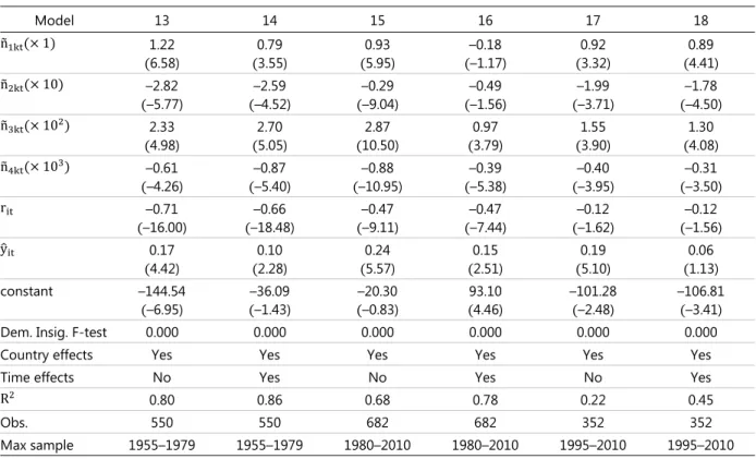
The demographic impact is present in all three subsamples (Table 3). The demographic effect is clearly present in the 1955-1979 subsample, both when estimating it without (Model 13) and with time fixed effects (Model 14). More interestingly, the demographic effect is present in the 1980-2010 subsample (Models 15 and 16) and even in the 1995-2010 subsample (Models 17 and 18). Though the estimated coefficients and the explanatory power of the benchmark regression decline somewhat in newer subsamples, the demographic effect remains very significant both statistically and economically.
It is not only impossible to get rid of the demographic effect, but even the age cohort specific effect is similar to the benchmark model (Graph A3 in the Appendix). The benchmark model (left-hand panel) and the 1995-2010 subsample (right-hand panel) show the same U-shape pattern for the inner age cohorts. As expected, the statistical significance is slightly weaker in the shorter subsample. Perhaps due to
this decreased precision the economic impact is also slightly lower. In any case, demography remains both statistically and economically highly significant.
Demography and inflation – robustness over time
Benchmark model, dependent variable is t Table 3
Model 13 14 15 16 17 18 n (× 1) 1.22 (6.58) (3.55) 0.79 (5.95) 0.93 (–1.17) –0.18 (3.32) 0.92 (4.41) 0.89 n (× 10) –2.82 (–5.77) (–4.52) –2.59 (–9.04) –0.29 (–1.56) –0.49 (–3.71) –1.99 (–4.50) –1.78 n (× 10 ) 2.33 (4.98) (5.05) 2.70 (10.50) 2.87 (3.79) 0.97 (3.90) 1.55 (4.08) 1.30 n (× 10 ) –0.61 (–4.26) (–5.40) –0.87 (–10.95) –0.88 (–5.38) –0.39 (–3.95) –0.40 (–3.50) –0.31 r –0.71 (–16.00) (–18.48) –0.66 (–9.11) –0.47 (–7.44) –0.47 (–1.62) –0.12 (–1.56) –0.12 y 0.17 (4.42) (2.28) 0.10 (5.57) 0.24 (2.51) 0.15 (5.10) 0.19 (1.13) 0.06 constant –144.54 (–6.95) (–1.43) –36.09 (–0.83) –20.30 (4.46) 93.10 –101.28 (–2.48) –106.81(–3.41)
Dem. Insig. F-test 0.000 0.000 0.000 0.000 0.000 0.000
Country effects Yes Yes Yes Yes Yes Yes
Time effects No Yes No Yes No Yes
R 0.80 0.86 0.68 0.78 0.22 0.45
Obs. 550 550 682 682 352 352
Max sample 1955–1979 1955–1979 1980–2010 1980–2010 1995–2010 1995–2010
Note: The estimates for the two oil crisis dummies in Model 13 are available upon request
Additional controls
The previous subsection demonstrated that the demographic impact remains robust to the choice of sample period. However, questions remain whether demography picks up the impact of some other observable variables. In order to control for such factors, we expand the benchmark model (equation 6) with additional variables and obtain the below specification:
= + + ∑ + + + 74 + 80 + + (7)
where is a vector that collects the controls.
Table 4 shows the results for four additional control variables. The first column (Model 19) just replicates the benchmark model for comparison. The first variable to add to the benchmark model is the growth in broad money (M2) relative to GDP, i.e. the change in the Marshallian K (Model 20). Importantly for our interest the demographic coefficients remain robust. The coefficient on money growth, however, is negative, suggesting that rapid monetary growth periods were associated with relatively low inflation, suggesting that the low inflation - high credit growth of the early-2000s might not have been unique. Second we add fiscal balance relative to GDP (Model 21). While the demographic impact remains robust, the fiscal balance also becomes statistically significant. The negative sign is also intuitive: higher fiscal deficits, after controlling for demography and real interest rates, are associated with higher inflation.
Demography and inflation – adding controls
Benchmark model, dependent variable is t Table 4
Model 19 20 21 22 23 24 (× 1) 1.91 (18.43) (11.19) 1.28 (6.69) 1.04 (6.24) 0.98 (7.52) 1.07 (0.21) 0.03 (× 10) –4.16 (–17.66) (–11.19) –2.80 (–9.37) –2.98 (–7.66) –2.35 (–9.86) –2.74 (–1.97) –0.06 (× 10 ) 3.26 (16.01) (10.26) 2.17 (10.30) 2.73 (8.03) 1.99 (10.43) 2.33 (3.21) 0.84 (× 10 ) –0.84 (–18.13) (–9.14) –0.55 (–10.26) –0.79 (–7.91) –0.55 (–10.06) –0.64 (–3.99) –0.30 –0.59 (–18.13) (–11.08) –0.46 (–7.86) –0.39 (–6.16) –0.30 (–6.64) –0.29 (–7.03) –0.38 0.15 (3.94) (3.99) 0.17 (6.09) 0.27 (6.01) 0.21 (8.31) 0.27 (4.72) 0.25 ∆( 2 / ) –0.06 (–2.48) (–0.32) –0.01 ( − )/ –0.07 (–2.74) (–0.65) –0.01 –0.00 (–0.02) (–1.72) –0.02 –0.01 (–2.70) (–3.42) –0.01 (0.31) 0.00 2.37 (3.49) (4.42) 3.01 (2.79) 223 3.87 (5.56) (5.40) 3.73 (5.56) 1.96 (3.82) 2.90 (2.90) 2.30 . –219.56 (–16.10) –129.81 (–3.60) (–1.52) –36.26 (–3.29) –82.94 –62.78 (2.73) (2.15) 48.45
Dem. Insig. F–test 0.000 0.000 0.000 0.000 0.000 0.000
Country effects Yes Yes Yes Yes Yes Yes
Time effects No No No No No Yes
0.62 0.56 0.69 0.68 0.65 0.79
Obs. 1232 981 603 740 556 784
Max sample 1955–2010 1955–2010 1980–2010 1970–2010 1980–2010 1970–2010
Finally, we include asset price inflation, ie residential property price growth and equity price growth, to implicitly account for wealth transfers between population cohorts. The inclusion of these variables is complicated by the fact that demography, more precisely the age structure of the population, might also drive real asset prices (Takáts, 2012). In principle, they could pick up the demographic impact even when demography is a driver of inflation. However, the inclusion of the two asset price growth rates leaves the demographic impact intact (Model 22). In fact, only equity price inflation comes out significant with a slightly surprising negative sign: ie stock market booms are associated with lower inflation. Again, these results suggest that the United States’ experience in the early-2000s, with booming stock markets and low inflation, were not entirely unique. The strength of equity price inflation in explaining consumer goods inflation is confirmed when all four control variables are included at the same time (Model 23). In this case only the equity price inflation variable remains significant. However, the significance of equity price inflation disappears when time fixed effects are added to the model (Model 24). This implies that although equity prices might be relevant for explaining
inflation, the cross-country variation in equity price dynamics cannot meaningfully explain the evolution of inflation.
In sum, the additional control variables confirm the robustness of the demographic impact: in all specification the population polynomial remained statistically and economically significant. Furthermore, the estimated U-shape pattern across age cohorts has also remained stable.
Model dynamics
Given that we are matching frequency variation in inflation with equally low-frequency demographic movements, it is reasonable to check that the correlations presented are not spurious. We show in this subsection that demography remains statistically and economically significant after allowing for dynamics and transforming the data to stationarity.
To address concerns of spurious regression, we add lags of inflation, real interest rate and output gap to the right-hand side of the benchmark model (equation 6), lag the polynomial terms by one period, and rewrite the result in error correction form:
∆ = + + ∆ + ∆
− ( , − , − , − ∑ , ) + (8)
The term in parenthesis captures deviations from an empirical steady-state relationship between inflation and the real interest rate, the output gap and the population polynomial. This part of the equation has the same interpretation as the specifications that we have so far been estimating. The adjustment coefficient describes how fast deviations from the estimated steady-state translate into inflation growth. The remaining terms capture short-run dynamics. Note that we do not allow the population terms in (8) to have any short-term effects since we did not add lags of the population polynomial to the equation.
The benefit of the specification in (8) is that the left-hand side variable is now clearly stationary. Consequently, only stationary right-hand side variables can be relevant for explaining it. For example, if it turns out that the regressions that we have so far conducted were spurious, the steady-state deviations would be non-stationary and, hence, should be zero.
Using the dynamic fixed effects (DFE) specification in (8) does not change the estimated demographic impact meaningfully (Table 5). Model 25 shows the estimates without time fixed effects and Model 26 with time fixed effects. The coefficient estimates for the polynomial terms are highly significant and are still very much in line with the benchmark results. Adding time fixed effects also has approximately the same effects as before, i.e. somewhat weakening but not eliminating the demographic impact. Moreover, in both cases the adjustment coefficient is both significant and negative, indicating that deviations from the long-run equilibrium error correct into inflation movements and that the errors are mean reverting. Taken together, these results imply that the population effects are not spurious.
However, the large coefficients on the output gap in models 25 and 26 might be puzzling at first glance. There are two relevant considerations for this impact. First, the magnitude of the effect on per-period inflation growth should be multiplied with : this multiple is much smaller and much more in line with what we
had before. Second and more importantly, the output gap captures cyclical fluctuations of a much higher frequency than demography or low-frequency inflation. Consequently, the high coefficient value probably indicates that the output gap does not belong in the long-run relationship. In other words, the swings in the output gap are so fast that the estimated large long-run effect never has time to materialize. Further reinforces this argument the fact that the coefficients on the output gap in Models 25-30 seem to fluctuate inversely with the adjustment coefficient .
Country heterogeneity
An additional concern is whether the homogeneity assumptions underlying the panel regressions are approximately satisfied. To dispel these concerns we show that country heterogeneity does not meaningfully affect the demographic impact. We first allow all short-run coefficients and the adjustment coefficient to vary with the country index, i.e. we estimate these models by the pooled mean group (PMG) estimator derived in Pesaran and Smith (1995). We then allow for full heterogeneity with respect to all the coefficients, i.e. we use the mean group (MG) estimator derived in Pesaran et al (1999).
Demography and inflation: dynamics and heterogeneity
Benchmark model, dependent variable: t Table 5
Model 25 26 27 28 29 30
Estimator DFE DFE PMG MG PMG PMG
(× 1) 2.17 (7.22) (1.15) 0.31 (8.36) 1.86 (2.55) 1.95 (4.24) 4.15 (10.82) 2.16 (× 10) –5.16 (–6.25) (–3.07) –1.53 (–8.01) –4.24 (–2.02) –4.24 (–4.41) –9.80 (–10.14) –4.98 (× 10 ) 4.35 (5.46) (4.26) 1.72 (7.23) 3.43 (1.37) 2.83 (4.13) 8.06 (9.13) 4.13 (× 10 ) –1.20 (–4.89) (–4.08) –0.57 (–6.51) –0.91 (–0.80) –0.53 (–3.69) –2.15 (–8.29) –1.12 –0.72 (–5.18) (–8.97) –0.66 (–10.18) –0.63 (–4.83) –0.72 (–5.05) –1.77 (–6.02) –0.41 1.68 (4.07) (6.84) 0.85 (9.47) 1.57 (5.22) 0.99 (3.78) 3.22 (9.06) 1.20 − –0.16 (–3.73) (–5.45) –0.24 (–13.28) –0.19 (–11.40) –0.46 (–6.32) –0.07 (–10.58) –0.26 ∆ –0.66 (–20.67) (–21.10) –0.66 (–15.97) –0.59 (–12.55) –0.57 (–12.44) –0.70 (–10.83) –0.53 ∆ 0.21 (5.63) (2.88) 0.09 (7.64) 0.25 (4.44) 0.18 (3.02) 0.22 (7.16) 0.26 . –34.46 (–4.04) (–4.04) –34.46 (–13.29) –35.28 (–1.65) –63.05 (–6.37) –29.34 (–10.63) –59.68 Dem. Insig. F–test 0.000 0.000 0.000 0.000 0.000 0.000
Country effects Yes Yes NA NA NA NA
Time effects No Yes NA NA NA NA
0.73 0.81 NA NA NA NA
Obs. 1232 1232 1232 1232 448 784
Max sample 1955–2010 1955–2010 1955–2010 1955–2010 1955–2010,
The demographic impact remains both statistically and economically significant after adding country heterogeneity (Models 27 and 28, Table 5). Again the coefficients are similar to those of the benchmark model and are highly significant. Moreover, the PMG estimator generates a very similar U-shaped age cohort effect on inflation as the benchmark model (left-hand panel, Graph A4 in the Appendix). The basic U-shape pattern also remains in the MG estimator, but the form moves closer to a second order polynomial (right-hand panel). However, one should treat this result somewhat cautiously because the impact of the very young and the very old cohorts drive the pattern, which are potentially imprecisely estimated.
One benefit of the MG estimator is that it produces country specific estimates of the steady-state as a byproduct. This allows us to check how individual countries behave in the panel. Put it differently, if the estimates of the steady-state coefficients vary a lot across countries, then a different country grouping might overturn the results.
The individual country estimates of the benchmark model reveal a surprising degree of homogeneity with respect to the long-run relationship (Table 6). To see this, note that two general patterns go through the estimates. First, going from the lower order polynomial terms to the higher order ones, the coefficients tend to alternate in sign. In the vast majority of countries, the first coefficient is positive, the next negative and so on. The pattern is reversed in five countries (Denmark, Japan, Korea, the Netherlands and Spain),3 whereas the alternation is broken in only two
cases (Finland and Portugal). A second similarity between the countries is that the coefficients on the second and third order terms are approximately twice as large as the coefficients on the first and fourth order terms. The biggest difference between the countries appears to be the relative magnitude of the coefficients, rather than their internal relationship. This suggests that the long-run relationships across countries differ from each other primarily by a constant, possibly negative, scaling factor. This would explain why the panel estimates generated such a good fit when compared to the inflation experiences in the individual countries (Graph 3 and 5).
Table 6 also reveals that the steady-state deviations appear to be significantly mean reverting in most countries. The adjustment coefficients are insignificant in only three countries (Greece, Italy and Portugal) – and even in these cases, it should be kept in mind that the estimates for each country is based on only 55 observations. The population polynomial is only insignificant in the case of Portugal.
Despite the similarities across countries, it might be worthwhile to split the sample and apply the PMG estimator on different groups as an additional robustness check (Models 29 and 30, Table 5). In order to obtain two as different country sets as possible in terms of demographic impact, we split the sample into one group consisting of the countries where the results seem to be the weakest (Greece, Italy, and Portugal) or where the parameter sequence deviates from the dominant pattern (Denmark, Finland, Japan, Korea, the Netherlands and Spain) and another consisting of the remaining countries. That is, we separately estimate the population polynomial for the set of countries where results are likely to be the weakest (Group I – Model 29) and for the set where results can be expected to be
3 The reversal in the alternation of the polynomial coefficients does not appear to change the implied
population coefficients. The MG estimator for these five countries produces the same pattern as in the benchmark model, again except for the very young and the very old.
the strongest (Group II – Model 30). Impressively, the long-run relationship between demographics and inflation appears to be almost identical between the two groups, aside from different scaling. Again, the polynomial coefficients are very significant and show a similar pattern. In sum, re-estimating our regression on the group of countries which are the most different in terms of the population polynomial estimates does not yield meaningfully different results from the benchmark model.
Demography and inflation: country specific estimates Table 6
(× 1) (× 10) (× 10 ) (× 10 ) − F(4,1250) AT 0.02 (0.04) (–0.38) –0.40 (0.36) 0.32 (–0.18) –0.05 (–5.42) –0.66 0.000 AU 5.98 (5.99) (–5.48) –13.82 (5.05) 12.88 (–4.79) –4.05 (–4.90) –0.60 0.000 BE 2.03 (0.88) (–0.83) –4.61 (0.73) 3.80 (–0.65) –1.03 (–3.15) –0.42 0.000 CA 1.25 (1.47) (–0.86) –2.24 (0.39) 1.20 (–0.12) –0.14 (–3.01) –0.40 0.000 CH 1.10 (2.26) (–2.12) –2.35 (1.78) 1.77 (–1.47) –0.44 (–5.17) –0.64 0.000 DE 0.18 (0.31) (–0.49) –0.66 (0.44) 0.53 (–0.32) –0.11 (–4.74) –0.45 0.000 DK –0.66 (–0.81) (0.35) 0.55 (–0.64) –0.86 (1.21) 0.49 (–4.95) –0.76 0.000 ES –0.55 (–0.45) (0.39) 1.29 (–0.86) –3.43 (1.22) 1.83 (–4.37) –0.48 0.000 FI 0.57 (1.04) (–0.15) –0.20 (–0.54) –0.63 (0.87) 0.35 (–3.00) –0.38 0.000 FR 4.26 (1.41) (–1.31) –9.01 (1.20) 7.32 (–1.11) –2.01 (–2.70) –0.34 0.000 GB 2.24 (3.25) (–3.19) –5.00 (2.54) 3.75 (–1.97) –0.90 (–4.25) –0.52 0.000 GR 9.92 (3.19) (–3.71) –29.51 (3.79) 26.82 (–3.66) –7.45 (–1.74) –0.11 0.002 IE 4.41 (1.40) (–1.35) –10.47 (1.24) 9.21 (–1.14) –2.69 (–4.22) –0.54 0.000 IT 8.04 (2.55) (–2.86) –18.05 (2.66) 14.08 (–2.14) –3.53 (–0.99) –0.12 0.037 JP –0.47 (–0.74) (1.19) 1.78 (–1.44) –1.98 (1.56) 0.66 (–3.95) –0.54 0.000 KR –7.67 (–1.70) (1.75) 24.31 (–1.80) –27.45 (1.82) 9.71 (–3.80) –0.33 0.000 NL –1.56 (–1.09) (1.13) 3.72 (–1.28) –4.06 (1.42) 1.48 (–3.34) –0.43 0.000 NO 2.36 (4.35) (–5.13) –4.75 (4.69) 3.42 (–3.74) –0.82 (–4.58) –0.66 0.000 NZ 3.99 (5.10) (–4.48) –8.96 (3.88) 8.18 (–3.46) –2.57 (–5.70) –0.72 0.000 PT 2.86 (0.64) (–0.51) –5.59 (0.09) 1.14 (0.19) 0.95 (–0.98) –0.08 0.211 SE 3.30 (4.03) (–4.89) –6.83 (4.22) 4.67 (–3.08) –1.00 (–3.35) –0.49 0.000 US 1.26 (1.87) (–1.65) –2.41 (1.15) 1.61 (–0.76) –0.35 (–2.58) –0.39 0.000
Demography and monetary policy
The evidence presented so far suggests that demographic change affects low-frequency inflation beyond the impact of other factors, including that of short-term real interest rates. This pattern raises questions about how and through which mechanism age structure could affect inflation.
In order to explore this we investigate whether the age structure is also related to the conduct of monetary policy, i.e. to real interest rate setting and to deviations from Taylor rules. The age cohort impact on these variables can also inform us whether monetary policy leans against inflationary pressures. If, for instance, monetary policy leans against the demographic impact, then one should see a similar U-shape age cohort effect emerge that we have seen with inflation. In other words, when the central bank leans against the demographic inflationary pressure, real interest rates, or deviations from Taylor rules, tend to be higher when the share of young and old is larger - and lower when the share of the working age cohorts is larger. Conversely, if monetary policy exacerbates the inflationary impact of demography one would expect a reverse U-shape pattern to emerge.
Age structure and real interest rates
We first show that the age structure of the population also does affect the short-term real interest rates. Building on the population polynomial setup from the previous section, we estimate the following specification for the ex-post real interest rate:4
= + + ∑ + (9)
The regression results confirm that demography affects the real interest rates (Table 7). The first column, Model 31, shows the results for the full sample. Demography is statistically and economically significant – and it accounts for more than one-eighth of the total variation of low frequency real interest rates.
Naturally, one also would need to control for those factors that monetary policy should have taken into account when setting the interest rates and investigate whether deviations from such an optimal policy are related to demography. For our analysis we will apply versions of the widely used Taylor rule to proxy optimal monetary policy. Furthermore, the Taylor rule is straightforward to calculate and can be used throughout the sample. However, we acknowledge that central bank decision making is complex, and straightforward rules might not be perfect proxies for optimal policies. Investigating the demographic effects on other rules is a natural future extension of our work.
Deviations from Taylor rules are also statistically significantly correlated with demography (Table 7, Models 32-34). We consider three Taylor rules. First, we
4 Adding time fixed effects has similar results as in the case of inflation. In particular, it does not
qualitatively change the demographic impact on real interest rates, but weakens the statistical significance and reduces the economic impact weaker by removing time variation. For the sake of brevity, the results with time fixed effects are not shown here, but are available upon request.
investigate deviations from the normative Taylor rule that Taylor (1993) originally suggested to describe US policy rates (Model 33). Next, we look at deviations from an empirically estimated Taylor-rule. In the first version we estimate a single Taylor rule for all countries in the sample (Model 34), and in the second version we allow the Taylor coefficients to vary across countries (Model 35). When estimating the Taylor coefficients we use the 1985-2010 period when there is more agreement that policy rates roughly followed such rules. Demography is again significant: deviations from normative and estimated Taylor rules all correlate statistically significantly with demography.
Demography, real interest rates and deviations from Taylor rules Table 7
Model 31 32 33 34 Dependent variable − 1.5 − 0.5 − − − − − − (× 1) 0.10 (0.63) (–3.91) –0.88 (–2.54) –0.49 (–2.80) –0.75 (× 10) 0.42 (1.23) (5.71) 2.77 (4.45) 1.83 (4.35) 2.44 (× 10 ) –0.77 (–2.64) (–6.66) –2.76 (–5.58) –1.95 (–5.14) –2.43 (× 10 ) 0.29 (3.55) (7.05) 0.85 (6.12) 0.62 (5.43) 0.74 constant –48.56 (–1.99) (1.55) 50.88 (0.34) 9.94 (0.67) 27.32 Dem. Insig. F–test 0.000 0.000 0.000 0.000
Country effects Yes Yes Yes Yes
Time effects No No No No
0.13 0.13 0.14 0.14
Obs. 1232 1232 1232 1232
Sample 1955–2010 1955–2010 1955–2010 1955–2010
The impact of age structure on real interest rates and deviations of real interest rates from Taylor rules follows an inverse U-shape pattern (Graph 5). The young and the old are associated with lower, while the middle-aged with higher real interest rates (left-hand panel). Similarly, the young and the old are associated with policy rates below the Taylor rule, while the working age population is associated with policy rates above the Taylor rule (right-hand panel). In sum, very similar U-shape pattern arises for real interest rates and deviations from Taylor rules.
Taken together with earlier results, the findings on interest rates suggest that monetary policy reinforced the impact of demography on inflation over the full sample. The reason is that demography drives the real interest down exactly when it drives inflation up (and vice versa). Hence, controlling for real interest rates eliminates an indirect demographic impact on inflation.
However, the conduct of monetary policy seems to have undergone a fundamental change around the mid-1980s. In particular, re-estimating real interest rates and deviations from Taylor rules for the 1955-1984 and the 1985-2010 period yields very different results (Table 8). In the first half of the sample we see the same qualitative picture emerging as for the full sample (Models 35 and 36 respectively). However, this pattern reverses completely in the second half of the sample (1985-2010): the coefficient estimates for both the real interest rate and deviations from the Taylor rule take the opposite sign as in the earlier part of the sample (Models 37
and 39 respectively). Importantly, the results do not disappear in the later period: they remain highly significant statistically – only their sign changes.
Age cohort effects on real interest rates and on deviations from the Taylor rule
1955-2010, in per cent Graph 5
Model 31 Model 34
In the first half of the sample (1955-1984), the demographic impact on monetary policy reinforced the demographic pressures on inflation. The young and the old are associated with lower real interest rates, while the working age with higher real interest rates (left-hand panel, Graph A5 in the Appendix). Similarly, the young and the old are associated with below Taylor rule rates, while the working age with above Taylor rule rates (right-hand panel).
Demographic effects on real interest rates and on deviations from Taylor rules Table 8
Model 35 36 37 38 Dependent variable − − − − − − (× 1) -1.09 (-4.00) (–4.06) –1.87 (7.04) 1.27 (2.70) 0.51 (× 10) 3.20 (4.94) (4.51) 4.91 (-6.73) -2.44 (-2.03) -0.77 (× 10 ) –3.16 (–5.40) (–4.64) –4.53 (5.57) 1.66 (0.93) 0.29 (× 10 ) 0.97 (5.56) (4.57) 1.32 (-4.37) -0.37 (0.05) 0.00 constant 102.05 (2.85) 200.62(3.35) -154.70(-5.33) (-2.10) -63.88 Dem. Insig. F–test 0.000 0.000 0.000 0.000
Country effects Yes Yes Yes Yes
Time effects No No No No
0.05 0.07 0.49 0.27
Obs. 660 660 572 572
Sample 1955–1984 1955–1984 1985–2010 1985–2010
In the second half of the sample (1985-2010), the reversal in estimated coefficients also implies a reversal in the age cohort effects: a U-shaped pattern emerges (Graph 6). In particular, real interest rates are higher when the
–1.0 –0.5 0.0 0.5 1.0 0–4 5–9 10–14 15–19 20–24 25–29 30–34 35–39 40–44 45–49 50–54 55–59 60–64 65–69 70–74 75–79 80+ +/-2 standard deviation –1.0 –0.5 0.0 0.5 1.0 0–4 5–9 10–14 15–19 20–24 25–29 30–34 35–39 40–44 45–49 50–54 55–59 60–64 65–69 70–74 75–79 80+
demographic pressure on inflation is strong and lower when the demographic pressure is weak, i.e. the young and old are associated with higher real rates and the working age with lower real rates (left-hand panel). The deviations from the Taylor rule follow a similar pattern: the young and the old are associated with higher real interest rates, while the working age with lower real interest rates (right-hand panel). In sum, central banks seem to have started to lean against demographic inflationary pressures in the 1980s.
Age cohort effects on real interest rates and on deviations from the Taylor rule
1985-2010, in per cent Graph 6
Model 37 Model 38
Potential drivers: modelling demographic pressures
Our empirical analysis shows a robust and stable empirical link between demography and inflation – and similarly a robust though unstable link between demographic structure and real interest rates. In this section, we first summarize the relevant empirical findings and then explore a theoretical model could explain them. Last, we discuss how to interpret the findings.
Stylised facts and theories
Our results show a robust and consistent correlation between demography and inflation and a shifting correlation between demography and monetary policy (Graph 8). As for the relationship between demography and inflation the same stable U-shaped pattern arises irrespective of the precise period or empirical technique chosen (black line): the young and the old are associated with higher rate of inflation, while the working age cohorts are associated with lower inflation rates.
As for monetary policy, we have seen a major shift between the first and second half of the sample - irrespective whether we measure monetary policy by real interest rates or by deviations from a Taylor rule. In the earlier part of the sample (1955-1984) monetary policy reinforced the demographic impact: central banks lowered the real interest rate when the demographic pressure was strong and increased the rate when the pressure was weak (left-hand panel, Graph 7).
–1.0 –0.5 0.0 0.5 1.0 0–4 5–9 10–14 15–19 20–24 25–29 30–34 35–39 40–44 45–49 50–54 55–59 60–64 65–69 70–74 75–79 80+ +/-2 standard deviation –1.0 –0.5 0.0 0.5 1.0 0–4 5–9 10–14 15–19 20–24 25–29 30–34 35–39 40–44 45–49 50–54 55–59 60–64 65–69 70–74 75–79 80+
Conversely, the pattern reversed in the second half of the sample during 1985-2010: monetary policy started to counter demographic pressures (right-hand panel).
Age cohort effects on inflation Graph 7
Taken at face value these empirical correlations are inconsistent with the textbook New Keynesian model. One problem, that we have already discussed, is the persistence of deviations from their explicit or implicit targets: making mistakes in 20 countries over 20 years stretches credibility. A deeper issue arises because our empirical analysis reveals that demography is correlated with inflation even after controlling for real interest rates and economic cycles: this suggests that inflation has an additional structural driver. One potential explanation is that demography drives the equilibrium real interest rate, i.e. the interest rate that stabilizes inflation – though even this explanation requires central banks to make consistent mistakes extremely persistently.
In order to better understand this issue we introduce a straightforward alternative model of demographic demand in the following subsection.
A model of demographic demand
Setup
The model combines lifecycle theory, dating back to Brumberg and Modigliani (1954) and Ando and Modigliani (1963), with overlapping generation, dating back to following Allais (1947), Samuelson (1958) and Diamond (1965). The model abstracts away from the actions of the central bank and uses an exogenously given money supply. As we show, the model can replicate the same pattern that we see in the early half of the dataset, i.e. when central banks did not offset the inflationary pressure from inflation. In particular, the young and the old are inflationary while the working age cohorts are deflationary. Furthermore, the young and the old raise the real interest rates, while working age cohorts reduce it.
In the economy, there is a continuum of overlapping generations. Agents live for three periods: young, working age, and old. The young and the old do not work, while the working age agents work and receive exogenous wage in perishable consumption goods (w). –1.0 –0.5 0.0 0.5 0–4 5–9 10–14 15–19 20–24 25–29 30–34 35–39 40–44 45–49 50–54 55–59 60–64 65–69 70–74 75–79 80+ Inflation (1955–2010, model 10)
Real interest rate (1955–1984, model 35)
–1.0 –0.5 0.0 0.5 0–4 5–9 10–14 15–19 20–24 25–29 30–34 35–39 40–44 45–49 50–54 55–59 60–64 65–69 70–74 75–79 80+ Inflation (1955–2010, model 10)
We focus on demographic change and we capture this change via the variable
k, which denotes the number of children each working age agent has (k>0). For
analytic simplicity we do not constrain k to be a natural number. Each working age person values the utility of their k children similarly to they own though with some discount (0<<1). The children consume only the transfers from their parents. Working age people also value their old age consumption with some time discount (0<<1) and save money to purchase perishable consumption goods later in old age. The stock of the total amount of money in the economy is set exogenously.
Finally, the long-term real return from holding money (r) is the relative price difference between consumption today and tomorrow. Agents’ utility function is logarithmic for analytic simplicity. Formally, at time t a working age agents utility maximization problem looks as follows:
max ln + ln + βE[ln ] (1)
where cY, cW and cO are young age, working and old age consumption,
respectively. E[.] denotes expectations. The utility maximization is subject to the individual budget constraint:
+ + ≤ (2)
Solution
Solving the individual problem can be done in two steps. First, we recognize that the ratio of marginal utilities between young and working age consumption equals with the ratio of relative prices, and the latter comes from (2) directly:
=
Notice that as the number of children (k) increases the model predicts that individual utility of each children decreases compared to that of the working age adult. This result arises due to the convexity of the utility function. Using this result we can obtain the ratio of young and working age consumption:
=
This expression, together with recognizing that the budget constraint always binds, allows rewriting the maximization problem as a function of cW only:
max ln + ln + βln (1 + )[ − (1 + ) ]
Taking the first order condition yields - after straightforward algebra - working age consumption:
= (3)
Substituting in yields young and old age consumption:
= (4)
[ ] = ( ) (5)
Old age consumption implies that saving for old age is
= (6)
The results show that agents spend a share of their wage income on children, themselves and on saving for old age. As under logarithmic utility the price and
income effects of real return (r) cancel each other out, the shares dedicated to these three categories do not depend on real interest rates.5 Consequently, rising wages
(ie working age income) affect young, working age and old age consumption the same way. Further comparative statics are also intuitive: having more children (larger k) results in less working age consumption, smaller savings for old age and smaller consumption by each individual child (cY) – but more consumption by all
children in the household (kcY). Stronger preference for the consumption of one’s
children () increases the consumption of children, but decreases both working age consumption and savings for old age.
We can also derive the price of consumption goods. Let’s introduce M as the exogenous stock of money, which equals in equilibrium with aggregate nominal savings, i.e. real savings multiplied with the price level p:
=
where is the number of working age individual whose individual savings are obtained from equation (6). Thus, the price level is given by:
= (7)
The impact on the price level is the opposite on the impact on money demand: larger working age groups or higher wages increase the price level and more children decrease the price level.
Steady state
Consider first the steady state economy where all generation at all times are of size
n and all k=1. Resource constraint (2) can then be written without the expectation
term formally as
+ + ≤
which yields – after simplifying with n and k=1 and substituting in consumption solutions (3), (4) and (5) – to the following formula:
(1 + (1 + ) + ) =
It is clear that r=0 represents the only solution for >0. Thus, in the steady state the real long-term rate of return is zero (r*=0).
The steady state price level follows from equation (7):
∗=
5 Technically, the fact that savings is independent of the interest rate simplifies the solution of the
model. We can take the solution from equations (3), (4) and (6) and directly plug the results back to the resource constraint. This yields the ex-post equilibrium real interest rate r in each period. Importantly, this implies that the expectations formed at each period about the real interest rate would not affect the optimization problem. Consequently, the solution to the problem is not dependent on whether the demographic change is expected or not.