Asset Pledgeability and
Endogenously Leveraged Bubbles
Julien Bengui
aToan Phan
b,cJune 18, 2018
a Université de Montréal & CIREQ, Canada b Federal Reserve Bank of Richmond, U.S.A. c VCREME, Vietnam
Emails: [email protected], [email protected]
Abstract
We develop a simple model of defaultable debt and rational bubbles in the price of an asset, which can be pledged as collateral in a competitive credit pool. When the asset pledgeability is low, the down payment is high, and bubble investment is unleveraged, as in a standard rational bubble model. When the pledgeability is high, the down payment is low, making it easier for leveraged borrowers to invest in the bubbly asset. As loans are packaged together into a competitive pool, the pricing of individual default risk may facilitate risk-taking. In equilibrium, credit-constrained borrowers may optimally choose a risky leveraged investment strategy – borrow to invest in the bubbly asset and default if the bubble bursts. The model predicts joint boom-bust cycles in asset prices and securitized credit.
Keywords: rational bubbles, collateral, credit pool, household debt, equilibrium default.
JEL codes: E12; E24; E44; G01
1
Introduction
This paper develops a tractable model of endogenously leveraged asset bubbles. The model aims to address several policy-relevant question for economic theory: Under what conditions might risky asset bubbles and risky debt end up on the balance sheets of agents who are
more likely to default? Under what conditions do asset bubbles become leveraged (i.e., in-vestment in the bubbly asset is financed by credit)? How do leveraged bubbly episodes differ from unleveraged ones? These questions are motivated by a concern among economists and policymakers that the boom and bust of leveraged asset bubbles can have serious macroe-conomic consequences (see, e.g., Mishkin, 2008, 2009; Rajan, 2011; Greenspan, 2013; Mian and Sufi, 2014; also see Jordà et al., 2015 for historical evidence supporting this notion).
To address these questions, we develop a simple model of leveraged bubbles, based on the rational bubble framework à la Samuelson (1958), Diamond (1965), and Tirole (1985). We introduce two types of households: borrowers and lenders. Households can extend credit to each other. However, borrowers cannot commit to future repayment and thus need to post collateral. If a borrower defaults, she loses fraction φ of the holding of the bubbly asset that she pledged as collateral and a fraction of her endowment (as in the case of recourse loans). Following many papers in the recent macro-finance literature (e.g., Boz and Mendoza, 2014 and Caballero and Farhi, 2015), we view an exogenous increase in this fraction φ as a parsimonious representation of the consequence of the recent financial developments that increased households’ ability to borrow against their housing wealth.
To capture the main features of a securitized debt market, we impose an assumption that the borrowing and lending takes place via a competitive credit pool (Dubey et al., 2005). Debt issued by different borrowers is pooled together and sold as shares to lenders. By buying shares of the pool, lenders receive a pro rata share of the aggregated repayments (or garnishments in the case of default) by borrowers, in a manner similar to an investor in the securitized mortgage market. We assume that the pool is large so that individual borrowers and lenders take the debt price and delivery rate as given.
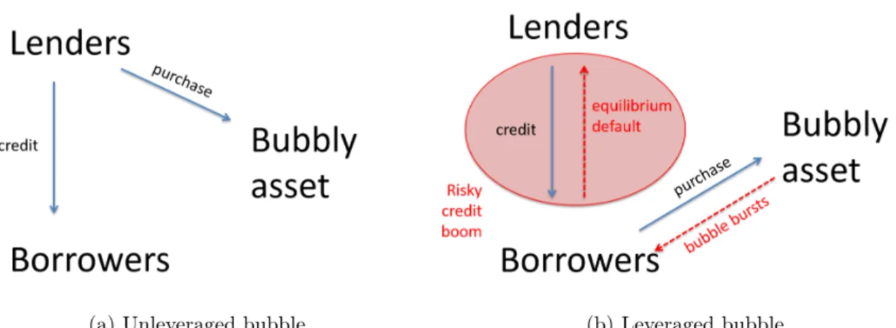
Our results point to a strong role of asset pledgeability and credit pooling in shaping the existence and characteristics of bubbly equilibria. When asset pledgeability is limited (φ is small), any equilibrium bubble is unleveraged: lenders buy the bubbly asset using their own funds, and the bubbly episode is not associated with a credit boom, as in a standard rational bubble model. Figure 1a illustrates an unleveraged bubbly equilibrium.
A contrasting set of results prevails when the bubbly asset is highly pledgeable (φ is high). In that scenario, any equilibrium bubble must be leveraged, as borrowers find an attractive return from leveraged investment (i.e., buying the bubbly asset using debt that is backed by the asset itself). The high pledgeability reduces the down payment for borrowers and the opportunity to default when the bubble bursts allows borrowers to shift some of the downside risk of bubble investment to lenders. In a standard bilateral loan contract, the price of debt (or equivalently, the interest rate) would internalize this shifting of risk. However, when loans are packaged together into a competitive credit pool, individual default
(a) Unleveraged bubble. (b) Leveraged bubble.
Figure 1: Bubble market participation and credit market interactions.
risks are also pooled together, facilitating the shifting of risk from borrowers to lenders. In fact, we show that when the pledgeability of the bubbly asset is high, any bubbly episode in equilibrium must be associated with leveraged investment and an expansion of lending in the credit pool. Hence, a distinguishing characteristic of leveraged bubbly episodes is that they come with default risk: when the bubble collapses, it is optimal for debtors to default, because then the value of their collateral falls below the face value of their debt. Figure 1b illustrates a leveraged bubbly equilibrium.
Our results also imply that the upper bound on the risk of bursting for a bubble to exist in equilibrium is more relaxed when the asset pledgeability is high. In other words, our model predicts that leveraged bubbles can be riskier than unleveraged ones. It also predicts that very risky bubbles can only exist if they are leveraged.
Our theory thus predicts that the combination of credit pools and a high degree of bub-bly asset pledgeability can facilitate the emergence of highly risky bubble episodes. One interpretation of the implication is that “easy credit,” loosely defined as lax down payment requirements combined with the packaging of risky loans into securitized credit pools, not only facilitates asset bubbles and credit booms, but can also change the nature of asset bub-bles from unleveraged to leveraged. Furthermore, in a leveraged bubbly episode, the risky bubbly asset ends up in the hands of agents who are prone to defaulting (the borrowers in our model). These predictions are qualitatively consistent with the narratives of the recent leveraged bubble episode in the U.S., which experienced a boom in securitized mortgage and debt-financed homeownership, following a period of drastic financial innovation and deregu-lation (Cooper, 2009 and Mian and Sufi, 2011, 2014). When asset prices began to falter in 2006, the credit boom turned into a bust, with widespread default and foreclosures (Mian and Sufi, 2009 and Barlevy and Fisher, 2011). Other leveraged bubble episodes in recent
history that began with periods of easy credit and ended with financial crises include those in Japan in the 1980s and early 1990s, in East Asian economies in the period leading up to the East Asian crisis, and in Ireland in the 2000s.1
Related literature. Our paper mainly relates to the literature on rational bubbles, which builds on the seminal contributions of Samuelson (1958), Diamond (1965), and Tirole (1985). It relates in particular to the modeling of stochastic bubbles by Weil (1987).2 Most relevant
is the recent stream of rational bubble models with financial frictions, such as Kocherlakota (2009), Miao et al. (2011; 2014; 2015), Arce and López-Salido (2011), Farhi and Tirole (2012), Martin and Ventura (2012; 2016), Aoki and Nikolov (2015), Zhao (2015), Basco (2016), and Hirano et al. (2015; 2016). Our work is closest to Miao and Wang (2011) and Martin and Ventura (2016), who also consider the possibility that bubbly assets provide collateral value to credit-constrained agents. Unlike us, however, they do not allow for equilibrium default, which plays a key role in shaping the difference in characteristics between leveraged and unleveraged bubbles in our framework. Furthermore, while they focus on the effects of bubbles on aggregate investment and activity, we focus on the effects of asset pledgeability on the existence of bubbles and on the profile of bubbly asset holders.
Existing papers that study leveraged bubbles and emphasize the role of risk shifting include Allen and Gorton (1993), Allen and Gale (2000), Barlevy (2014), and Ikeda and Phan (2016). A common assumption in these papers is that bubbly asset purchase is financed by credit. Therefore, in these papers, bubbles are leveraged by construction and risk shifting always occurs in equilibrium. In contrast, in our model, whether bubbles are leveraged and whether risk shifting occurs are endogenous outcomes of the interaction between the asset and credit markets and crucially depend on the degree of pledgeability of the bubbly asset. This endogeneity allows us to jointly analyze and compare leveraged versus unleveraged bubbly episodes.
To the best of our knowledge, our paper is the first to combine the rational bubbles framework with the general equilibrium framework with default and credit pool as developed by Dubey and Geanakoplos (2002) and Dubey et al. (2005). This combination allows our paper to analyze the interaction between asset price bubbles and securitized debt.
1See Hunter et al. (2005) and Shioji (2013). See also Herring and Wachter (1999) for a narrative of the
role of financial deregulation in the boom-bust cycles of collateralized lending and asset prices in Japan and Thailand. See Kelly (2009) and Connor et al. (2012) for narratives of the Irish bubble, including the role of loose credit conditions (including to some extent securitization and loose regulations of banks) that may have facilitated risky credit pools.
2For recent surveys of the literature, see Barlevy (2012), Miao (2014), and Martin and Ventura (2017).
For complementary approaches to rational bubbles, see Abreu and Brunnermeier (2003), Doblas-Madrid and Lansing (2014) and references therein.
Our paper borrows insights from the macroeconomic literatures on financial frictions (Bernanke and Gertler, 1989; Kiyotaki and Moore, 1997; Aiyagari and Gertler, 1999). We exploit the idea, notably present in Kiyotaki and Moore (1997), that limited enforcement and collateral constraints can generate a feedback loop between credit and asset prices. The main difference is that our model features equilibrium default. Our modeling of collateral constraints with equilibrium default is related to the models of collateral general equilibria (Geanakoplos, 1997; Geanakoplos and Zame, 2002; Simsek, 2013), except that we allow for recourse loans. Our paper can also be related to several papers that study how an asset’s pledgeability affects its market value (see, inter alia, Cipriani et al., 2012; Fostel and Geanakoplos, 2012).
Finally, our paper provides a leveraged bubble theory that is motivated by and is largely consistent with the empirical findings on bubbles and crises. Kindleberger and Aliber (2005) and Mian and Sufi (2014) argue that asset price booms depend on the growth of credit, and Jordà et al. (2015) find that leveraged bubbles in asset prices are more likely to be associated with financial crises than unleveraged ones.
The rest of the paper is organized as follows. Section 2 lays out the environment. Section 3 analyzes the bubbleless benchmark. Section 4 studies the unleveraged bubbly equilibrium, while Section 5 studies the leveraged bubbly equilibrium. Section 6 provides discussions and extensions, and Section 7 concludes. Proofs and detailed derivations are provided in the appendix.
2
Environment
Agents and endowment: Consider an economy with overlapping generations and perfect information. Time is discrete and infinite, denoted by t “ 0, 1, 2 . . . . There is a single per-ishable consumption good. Each generation consists of a continuous unit mass of individuals, whom we label borrowers (B), and a continuous unit mass of individuals, whom we label lenders (L). Agents live for two periods, labeled young age and old age. Each agent of type j P tB, Lu receives an endowment of ej0 when young and ej1 when old. We assume that lenders can commit to repaying debt in the future, but borrowers cannot. Thus, borrowers are naturally more prone to defaulting. (We relax this assumption in Section 6.)
Parametrization: An agent’s expected lifetime utility is given by EtrU pcj0,t, c
j
1,t`1qs “ Etrlnpcj0,tq ` lnpc j 1,t`1qs,
factor has been normalized to unity. For simplicity, we assume endowment profiles given by eB
0 “ 0, eB1 “ 1 and eL0 “ 1, eL1 “ 0. This parametrization is a simple way to generate a
strong motive for borrowing and lending and allows for tractable closed-form solutions.3
Agents can trade in two markets: the bubbly asset market and the credit market. We describe each of them below.
Bubbly asset market: We model bubbles in asset prices by following the conventional approach of the rational bubble literature. We assume that there is a competitive market where agents can trade (but cannot short-sell) a perfectly divisible and durable asset that is available in a fixed unit supply. The asset is bubbly in the sense that it pays no dividend but it may be traded at a positive price in equilibrium. As is standard in the literature (e.g., Kocherlakota, 2009; Martin and Ventura, 2012; Miao et al., 2014), we interpret the bubble as representing the difference between the market price of an asset, such as land and housing, and what could be considered its fundamental value, such as the net present value of land or housing rents (see Section 6.2.2 for an extension that formalizes this point).
Bubbles are inherently fragile as they require a coordination in expectations across agents: an agent is willing to buy the bubbly asset only if she expects to be able to resell it to someone else in the future. To model this fragility, we follow Weil (1987) and assume that in each period, the price of the bubbly asset can exogenously and permanently collapse to zero with a constant probability π P p0, 1q. Formally, we denote the price of one unit of the bubbly asset in period t by
˜
Pt” ξtPt,
where Ptis the bubble price conditional on the bubble having not collapsed, and tξtu8t“0 is a
process of binary random variables representing whether the bubble persists (ξt“ 1) or has
collapsed (ξt“ 0), which satisfies:
Prpξt`1“ 0|ξt“ 1q “ π
Prpξt`1“ 0|ξt“ 0q “ 1.
The first equation states that if the bubble has not collapsed in period t, then it will collapse in period t ` 1 with probability π. The second equation states that once the bubble has collapsed, agents expect that it will not reemerge. In each period t, agents trade the asset after learning the ξt shock. In each period, we call the state where the bubble persists the
good state and the state where it collapses the bad state. For simplicity, the bubble risk is the only source of risk in the model. As is standard, we assume that all of the bubbly asset
3For more general parametrizations, our results can be obtained numerically. What is essential is that the
belongs to the old generation at t “ 0.
Competitive credit pool: One of our main goals is to study the interaction between secu-ritized debt and asset price bubbles, which arguably played an important role in the 2007 financial crisis. To model the pool of securitized debt, we follow the seminal approach of Dubey et al. (2005). We think of mortgages as promises that borrowing homeowners sell to banks, who then sell the promises to investors through mortgage pools in the financial market. Banks play an intermediary role in verifying the credit limit of borrowers according to the eligibility criteria specified by the pool and in collecting and transferring payments from borrowers to shareholders of the pool. As in Dubey and Geanakoplos (2002) and Dubey et al. (2005), we abstract away from this intermediary role of banks and instead focus on the largely anonymous market interactions between the buyers (lenders) and sellers (borrowers) through the credit pool.
Formally, we assume that borrowers and lenders cannot trade bilaterally but can trade through an anonymous competitive credit pool. The pool is characterized by (i) a competitive price, (ii) a garnishment rule, and (iii) a credit limit.
(i) Competitive price: A young borrower i can borrow by selling di ě 0 units of debt into the pool, with each unit representing a promise to repay one unit of the consumption good in the subsequent period (when she is old). A lender i can lend by buying li units of promises from the pool. All trades take place in a competitive market where individual buyers and sellers are so small that they take as given the market price q of each unit of debt (or equivalently, the face-value interest rate 1{q). Of course, in equilibrium, the price that clears the market will incorporate the credit limit, the default risk, and the garnishment rule (specified below).
Note that this credit pool setup is very different from a setup in which borrowing takes place via a bilateral interaction between a borrower and a lender, where the price of debt (or equivalently, the face-value interest rate on a loan) is an explicit function of the amount that the borrower borrows. This implies that the default risk of a borrower is not individually priced but is instead priced only after it is pooled with the default risks of other borrowers in the market. With this price-taking assumption, we have in mind situations where home-owners can take out mortgages at interest rates that are relatively inelastic in the amount of debt, as long as the amount conforms with the credit limit specified by the credit pool (see point (iii) below). In Section 6.1, we show how the results change if instead borrowing takes place via bilateral interaction and prices are elastic in the amount of debt (as in, for example, the sovereign debt literature).
(ii) Garnishment rule: A borrower may choose to default on her promise. In the case of default, we assume that a fraction D P p0, 1q of the borrower’s old-age endowment (which was
normalized to one) and a fraction φ P r0, 1s of her holding of the bubbly asset are garnished and distributed proportionally to the buyers of the promise. Thus, the actual repayment in period t ` 1 of di
t promises that are issued in period t by a borrower is a random variable
that depends on the price of the bubbly asset and is given by: ˜
δt`1i “ mintdit, D ` φ ˜Pt`1aitu. (1)
Each buyer of promises in the credit pool receives a pro rata share of aggregated repay-ments/garnishments. The delivery rate at t ` 1 on a unit of debt issued at t is thus given by: ˜ ∆t`1 “ ş iPIB ˜δ i t`1 ş iPILl j t . (2)
Given this delivery rate, lenders who buy into the credit pool do not need to know the identity of the borrowers nor the quantities of their sales.
Remark: The fact that D ą 0 means debt has recourse, i.e., in the case of default, borrowers lose not only the collateral, but also some of their income. This assumption will be relevant in the leveraged bubbly equilibrium, as it implies that lending in the credit pool and investing in the bubbly asset yield different payoff structures – the former still yields a positive payoff in the state where the bubble collapses and borrowers default, while the latter does not. The assumption is also consistent with the fact that much of mortgage debt in the U.S. comes with recourse, as documented by Ghent and Kudlyak (2011).
(iii) Credit limit: We assume that each individual borrower i who participates in the credit pool is subject to a credit limit:
ditď D ` φ maxt ˜Pt`1uait,
or equivalently:
dit ď D ` φPt`1ait, (3)
where recall that Pt`1is the price of the bubble conditional on having not collapsed. Lenders
know that each individual borrower is subject to this credit limit. One can interpret this credit limit as being set by a regulator and being enforced by banks, which play the inter-mediary role of buying promises from borrowers and then selling to investors but are not modeled explicitly here. This credit limit rules out pathological equilibria in which borrowers incur so much debt that they will always default in equilibrium. The assumption that agents are subject to a credit limit while taking the price of debt as given is standard in the general equilibrium models with credit pool of Dubey and Geanakoplos (2002) and Dubey et al.
(2005). With this assumption, we have in mind, for example, the credit limits on conforming mortgage loans.
Note that in the polar case where φ “ 0, the credit limit (3) reduces to the simple debt limit in the standard general equilibrium models with incomplete markets of Bewley (1977), Huggett (1993), and Aiyagari (1994). In the other polar case where φ “ 1 and D “ 0, the credit limit corresponds to the credit limit on non-recourse loans that are often analyzed in the collateral equilibrium literature (e.g., Geanakoplos, 2010; Geanakoplos and Zame, 2014). Optimization problems: Taking prices as given, each borrower i chooses a portfolio of bubbly asset holding and debt to solve:
max aB,it ě0,ditě0 EtrU pc B,i 0,t, c B,i 1,t`1qs (4)
subject to budget constraints: cB,i0,t ` ξtPtaB,it “ qtdit cB,i1,t`1 “ 1 ` ξt`1Pt`1a B,i t ´ mintd i t, D ` φξt`1Pt`1a B,i t u,
and the credit limit (3).
Taking prices and the delivery rate as given, each lender j chooses a portfolio of bubbly asset holding and lending to solve:
max aL,it ě0,ljtě0 EtrU pc L,i 0,t, c L,i 1,t`1qs (5)
subject to budget constraints:
cL,i0,t ` ξtPtaL,it ` qtltj “ 1 cL,i1,t`1 “ ξt`1Pt`1a L,i t ` ˜∆t`1l j t.
Note that we have implicitly assumed in problem (4) that borrowers do not lend and in problem (5) that lenders do not borrow. This is without loss of generality, because under the parametrization of the endowment paths that we consider, borrowers never want to lend and lenders never want to borrow in equilibrium.
Since our analysis focuses on symmetric and stationary equilibria featuring time-invariant prices and symmetric allocations, we omit time subscript and individual superscripts from this point onward.4
4As the model does not feature a state variable (like capital in the model of Tirole, 1985), the transitional
Definition 1. A (stationary) competitive equilibrium consists of (time-invariant) portfolio choices aB, aL, d, l, a price q per unit of debt in the credit pool, a delivery rate ˜∆, and a price
P of the unburst bubbly asset, which satisfy:
• Taking prices and delivery rate as given, the allocations (aB, d) and (aL, l) solve
opti-mization problems (4) of borrowers and (5) of lenders, correspondingly. • Trades in the bubbly asset market clear: aB
` aL“ 1 if P ą 0; • Trades in the credit pool clear: d “ l;
• Trades in the consumption good market clear: cB
0 ` cB1 ` cL0 ` cL1 “ 2;
• The delivery rate satisfies (2);
The equilibrium is called bubbleless if P “ 0 and is called bubbly if P ą 0.
3
Benchmark: Bubbleless equilibrium
It is useful to start with the bubbleless benchmark. There always exists a bubbleless equi-librium, where the price of the bubbly asset is P “ 0. In this equiequi-librium, as there is no bubble, the credit limit for borrowers is simply d ď D and debt is thus risk-free. There are two cases, depending on whether the borrowers’ credit limit binds.
3.1
Unconstrained borrowers
First, suppose that the recourse D is large enough that the borrowers’ credit limit does not bind. Then it is straightforward to see that in the bubbleless equilibrium, lenders and borrowers achieve perfect consumption smoothing: cB
0 “ cB1 “ 1{2 “ cL0 “ cL1. The
bubbleless economy thus achieves the first-best allocation. The (risk-free) interest rate is 1{q “ u1pcL
0q{u1pcL1q “ 1. The conjecture that the borrowers’ credit limit does not bind
is only verified if D ě 1{2. Hence, under that condition, since the economy exhibits dy-namic efficiency, reflected in the fact that the interest rate is equal to the growth rate of endowments, bubbly equilibria cannot exist.
3.2
Constrained borrowers
Next, suppose that the recourse D is small enough that the credit limit binds in equilibrium. In particular, suppose that
D ă 1
2. (6)
Then it is straightforward to see that in equilibrium, the consumption profiles of lenders and borrowers are given by:
cB0 “ qD, cB1 “ 1 ´ D,
and
cL0 “ 1 ´ qD, cL1 “ D, where the price of debt q solves the Euler equation of lenders:
1 q “ u1pcL 0q u1pcL 1q .
This equation yields a unique solution, given by qnb “ 1{2D, where the subscript stands for
“no bubble.” Equivalently, the (risk-free) interest rate in the bubbleless equilibrium is given by:
Rnb ”
1 qnb
“ 2D. (7)
For the remainder of the paper, we will maintain assumption (6) so that the borrowers’ credit limit binds in the bubbleless equilibrium. Under this assumption, the credit limit lowers the interest rate below the growth rate of the economy, thus enabling the possibility of bubbles.5
4
Unleveraged bubbly equilibrium
We now study the possibility of a bubbly equilibrium where only lenders invest in the bubbly asset. We call such a bubbly equilibrium unleveraged, as it is characterized by self-financed investment in the bubbly asset by lenders. In an equilibrium of this kind, the bubbly asset plays the standard role of an investment vehicle for agents who have a large demand for savings (lenders in our model), as in Samuelson (1958), Diamond (1965), and Tirole (1985). In the absence of bubbles, the supply of assets comes from borrowers, who issue debt through the credit market. However, the presence of the credit limit constrains borrowers’ ability to supply assets. The ensuing shortage of assets enables bubbles, which can arise to meet the
5In other words, the presence of credit limit can facilitate the existence of bubbles in economies that are
otherwise dynamically efficient. This is similar to the result in recent rational bubbles models, such as Miao and Wang (2011), Martin and Ventura (2012), Farhi and Tirole (2012), and Hirano and Yanagawa (2016).
savers’ excess demand for assets.
In the following, we construct an unleveraged equilibrium and argue that such an equi-librium exists when (a) the interest rate in the bubbleless economy (Rnb from the previous
section) is sufficiently low, and (b) the pledgeability parameter φ of the bubbly asset in the credit limit (3) is not too large, so that the bubbly asset has a low collateral value.
Since only lenders hold the bubbly asset in an unleveraged equilibrium, bubbly asset holdings by borrowers and lenders must respectively be given by:
aB “ 0, aL “ 1. (8)
Hence, borrowers’ credit limit (3) reduces to d ď D. Under assumption (6), this credit limit must bind.6 Equilibrium borrowing and lending must therefore be respectively given by:
d “ D, l “ ´D. (9)
Given the claimed bubbly asset and credit positions, the consumption profiles of borrowers and lenders are respectively given by:
cB0 “ qD, cB1 “ 1 ´ D. (10) cL0 “ 1 ´ P ´ qD, cL1 “ $ & % cL 1,h ” P ` D if bubble persists, cL1,l” D if bubble bursts. (11)
It is apparent from these consumption expressions that the risk associated with the bursting of the bubble is entirely held by lenders.
Since in an unleveraged bubbly equilibrium, lenders are the marginal holders of both the credit security and the bubbly asset, the equilibrium prices q and P are determined by their Euler equations. More precisely, they solve the system consisting of lenders’ Euler equation for lending via the (risk-free) credit pool and lenders’ Euler equation for the (risky) bubbly asset holdings: qu1 pcL0q “ p1 ´ πqu1pcL1,hq ` πu1pcL1,lq (12) P u1 pcL0q “ p1 ´ πqP u 1 pcL1,hq. (13)
Given the logarithmic utility function, equations (12) and (13) yield the following unique
6If the credit limit did not bind, the borrowers’ unconstrained Euler equation for loans would require
solution: P “ PU ” 1 ´ π 2 ´ D, (14) q “ qU ” 1 ` π 2D, (15)
where the subscript U stands for ‘unleveraged.’
For these allocation and prices to indeed constitute a bubbly equilibrium, two conditions need to be satisfied. First, the bubbly asset price PU must be positive. Second, individual
borrowers must not face an incentive to unilaterally deviate from their conjectured equi-librium choices by leveraging up to purchase the bubbly asset. While the first condition is familiar from the existing rational bubble literature, the second condition is novel and results from the combination of credit pools and the possibility to pledge the bubbly asset as collateral. We discuss these two conditions below.
First, from expression (14), PU is positive if and only if D ă p1 ´ πq{2. From equation
(7), this condition is equivalent to Rnb ă 1 ´ π. In other words, for an unleveraged bubbly
equilibrium to exist, the bubbleless economy must feature a sufficiently low interest rate – lower than the growth rate of the economy adjusted by the bubble’s risk of bursting. Intu-itively, for the such an equilibrium to arise, lenders must face a sufficiently severe shortage of investment opportunities in the bubbleless world, where credit market frictions prevent borrowers from fully absorbing the economy’s demand for savings. Equivalently, the condi-tion places an upper bound on how risky an unleveraged bubble can be, i.e., π ă 1 ´ Rnb.
This is because if the bubble is too risky, then it is not attractive as a savings vehicle for lenders and thus cannot arise in equilibrium.
Second, for the allocations and prices above to constitute an equilibrium, it must be that any individual borrower does not have an incentive to unilaterally deviate from the equilibrium strategy by investing in the bubbly asset market. To see why this possibility matters, despite borrowers having a steeper endowment path than lenders, it is useful to introduce the notion of the “leveraged return” from bubble speculation. Assuming that a borrower exhausts her credit limit in young age and invests in the bubbly asset, it is optimal for her to default in old age whenever the bubble collapses. For this borrower, a unit of bubble investment therefore entails a down payment of p1´φqUqPU in young age and delivers payoffs
of p1 ´ φqPU in the good state and 0 in the bad state in old age. Thus, conditional on the
bubble surviving, the borrower enjoys a leveraged return of p1 ´ φq{p1 ´ φqUq, which is
always strictly larger than the unleveraged return of PU{PU “ 1, given that qU ą 1 from
(15). If φ ă 1{qU, then the leveraged return is increasing in φ and is strictly larger than
unleveraged return, as the down payment is negative while the expected gain is positive. The difference between the return rates of leveraged and unleveraged bubble investment is a consequence of the credit pool: the (risky) debt issued by the deviating leveraged borrower is pooled together with the (risk-free) debt issued by other unleveraged borrowers, who are following the equilibrium strategy. Thus, the deviating borrower benefits from an “under-pricing” of default risk.7 This may incentivize the borrower to follow the deviation strategy
if φ is sufficiently large.
Formally, using hats to denote deviation strategies and assuming a binding credit limit ˆ
d “ D ` φPUˆa, an individual borrower’s deviation payoff is given by:
ˆ v ” max ˆ aą0 u pqlooooooooooooomooooooooooooonUD ´ p1 ´ φqUqPUˆaq ˆ cB 0 `p1 ´ πqu p1 ´ D ` p1 ´ φqPUˆaq looooooooooooomooooooooooooon ˆ cB 1,h `πu p1 ´ Dq looomooon ˆ cB 1,l .
This compares with an equilibrium borrower payoff of:
vB ” upqUDq ` up1 ´ Dq. (16)
In the appendix, we show that ˆv is increasing in the pledgeability parameter φ, and vB ě ˆv
if and only if φ ě φ, where:8
φ ” D p2 ´ πq p1 ´ 2Dq ` π
2
p2D ` πq p1 ´ 2D ` πDq. (17) We thus have the following result:
Proposition 1.
1. Any unleveraged bubbly equilibrium (i.e., a bubbly equilibrium where only lenders invest in the bubble), if it exists, is uniquely characterized by equations (8) to (15).
2. The unleveraged bubbly equilibrium exists if and only if two conditions are satisfied: (a) the bubbleless interest rate is sufficiently low:
2D loomoon
Rnb
ă 1 ´ π (18)
7The under-pricing is relative to the benchmark where loans are not pooled (Section 6). 8As long as the low interest rate condition R
nb ă 1 ´ π is satisfied, it is straightforward to verify that
(b) and the pledgeability parameter of the bubbly asset is not too high:
φ ď φ, (19)
where φ is defined in (17). Proof. Appendix A.1.
Remark 1. For simplicity, we have assumed that the shares of lenders and borrowers are equal. It would be straightforward to allow for these shares to be given by θ P p0, 1q and 1 ´ θ, respectively. In this case, the condition Rnb ă 1 ´ π would still apply, but the
equilibrium bubbleless interest rate would be given by Rnb “ 2θ{p1 ´ θq. A higher θ would
imply a higher demand for assets (supply of savings) in the bubbleless equilibrium, leading to a lower interest rate and thus an environment that is more prone to the existence of bubbles.
5
Leveraged bubbly equilibrium
We now analyze the possibility of an equilibrium where borrowers also invest in the bubbly asset (aB ą 0). We call this bubbly equilibrium leveraged, as it is characterized by the
investment in the bubbly asset by borrowers that is (in parts) financed by credit.
The following result establishes that in a leveraged bubbly equilibrium, borrowers’ credit limit must bind. The intuition is that, given the steep endowment path of borrowers and the assumption that the fundamental collateral D is small (D ă 1{2), it would be suboptimal for a borrower to buy the bubbly asset but not take advantage of its collateral service. Lemma 1. In any bubbly equilibrium where aB ą 0, the credit limit (3) must bind for borrowers.
Proof. Appendix A.2.
In the following, we construct a leveraged equilibrium, and argue that such an equilibrium exists when (a) the interest rate in the bubbleless economy is sufficiently low, and (b) the pledgeability parameter φ of the bubbly asset in the credit limit (3) is large enough, so that the bubbly asset has a high collateral value.
Given Lemma 1, the representative borrower’s equilibrium debt position is given by
d “ D ` φP aB, (20)
where P again denotes the equilibrium price of the bubbly asset in the good state where the bubble persists. Equation (20) necessarily implies that there must be default in equilibrium.
This is because the collapse of the bubble precipitates non-repayment from “underwater” borrowers, who find the face value of their debt d exceeding the cost of default D.
Market clearing conditions imply that the representative lender’s bubbly asset holding and net lending position are given by:
aL “ 1 ´ aB, l “ ´d. (21)
Given the portfolios and default decisions, the consumption profiles of borrowers and lenders are respectively given by:
cB0 “ qd ´ P aB, cB1 “ $ & % cB 1,h ” 1 ` P aB´ d cB 1,l” 1 ´ D (22) cL0 “ 1 ´ P aL´ qd, cL1 “ $ & % cL1,h ” P aL` d cL 1,l ” ∆l d (23)
where the delivery rate on debt ∆ is 100 percent in the good state and only partial in the bad state due to default:
∆ “ $ & % ∆h ” 1 if bubble persists ∆l ” Dd if bubble bursts . (24)
Hence, unlike in the unleveraged bubbly equilibrium, the risk associated with the bursting of the bubble is held by both lenders and borrowers.
By substituting the expression for debt (20), the consumption for borrowers in (22) can be rewritten as: cB0 “ qD ´ p1 ´ φqqP aB, cB1 “ $ & % cB 1,h “ 1 ` p1 ´ φqP aB´ D cB 1,l “ 1 ´ D . (25)
The borrowers’ first-order condition with respect to the bubbly asset holding is thus: p1 ´ φqqP u1pcB0q “ p1 ´ πqp1 ´ φqP u
1
pcB1,hq.
Intuitively, under the leveraged investment strategy, the down payment per unit of asset for borrowers is p1 ´ φqqP . In the good state where the bubble persists (which happens with probability 1 ´ π), the marginal payoff net of debt repayment is p1 ´ φqP . However, in the bad state where the bubble collapses (which happens with probability π), borrowers
default and get a marginal payoff of zero. Note that if borrowers could not default, then the marginal payoff in the bad state would be ´φP . By canceling P from both sides of the equation above, we get a simpler first-order condition:
p1 ´ φqqu1pcB0q “ p1 ´ πqp1 ´ φqu 1
pcB1,hq. (26)
On the other hand, the first-order condition with respect to lending of the lenders is: u1 pcL0q “ 1 q “ p1 ´ πqu1pcL1,hq ` πu 1 pcL1,lq‰ , (27)
and their first-order condition with respect to the bubbly asset holding, along with the complementary slackness condition on aL
ě 0, is: u1 pcL0q ě p1 ´ πqu 1 pcL1,hq, “ if a L ą 0. (28)
When (28) holds with strict inequality, only borrowers hold the bubbly asset in equi-librium (aB “ 1, aL “ 0). We call a bubbly equilibrium fully leveraged if this is the case. Otherwise, when (28) holds with equality, both borrowers and lenders hold the bubbly asset. We call a bubbly equilibrium partially leveraged if this is the case.
By substituting the consumption profiles into the three first-order conditions (26), (27), and (28), we get a system of three equations that determine the three unknown prices and quantity P, q, and aB.
When do the allocations and prices above constitute a bubbly equilibrium? As in the unleveraged case, there are two necessary and sufficient conditions. The first is a condition for P ą 0, which requires the bubbleless interest rate to be sufficiently low. In the appendix, we show that this condition is:
Rnb ă φ ` p1 ´ φqp1 ´ πq
D 1 ´ D.
The second is a condition on the pledgeability parameter φ. Intuitively, for the borrowers to take on the leveraged investment strategy, the down payment 1 ´ φq must be sufficiently low. In fact, we can show that their holding of the bubbly asset aB is an increasing function of φ, and aB is positive if and only if φ is above the threshold φ, as defined in equation (17)
of the unleveraged equilibrium section.
In the appendix, we show that as long as the two conditions above are satisfied, then each borrower does not have an incentive to unilaterally deviate from the equilibrium strategy of
leveraged investment. To see the intuition, suppose on the contrary that a certain borrower i were to make a unilateral deviation and choose a portfolio such that she has no incentive to default even in the bad state where the bubble collapses. Then, her individual borrowing is effectively free from the risk of default. In a bilateral loan contract, the price of debt issued by borrower i would rise relative to the prevailing equilibrium price (or equivalently, the interest rate would decrease relative to the equilibrium interest rate) to reflect the lower individual default risk. However, under the competitive credit pool, borrower i’s debt is pooled together with the risky debt of the other borrowers and is thus given the same equilibrium price. In other words, the safe debt unilaterally issued by borrower i is “under-priced” by the credit pool, leading to a disincentive for the borrower to follow this deviation strategy. Hence, in equilibrium, it is individually optimal for each borrower to follow the leveraged investment strategy.
The existence conditions are formalized in the following proposition: Proposition 2.
1. Any leveraged bubbly equilibrium (i.e., a bubbly equilibrium where aB ą 0), if it exists, is uniquely characterized by equations (20) to (28).
2. The leveraged bubbly equilibrium exists if and only if two conditions are satisfied: (a) the bubbleless interest rate is sufficiently low:
2D loomoon
Rnb
ă φ ` p1 ´ φqp1 ´ πq D
1 ´ D. (29)
(b) and the pledgeability parameter of the bubbly asset is sufficiently high:
φ ą φ, (30)
where φ is defined in (17). Proof. Appendix A.3.
Remark 2. In Appendix A.3, we further show that there exists φ such that when φ ě φ, the bubbly equilibrium is fully leveraged (aB “ 1, aL “ 0), and when φ ă φ ă φ, the bubbly equilibrium is partially leveraged (0 ă aB, aLă 1). We will revisit this in the next section.
5.1
Comparison of bubbly equilibria and comparative statics
As a corollary of proposition 2, we can show that the price of the bubbly asset, the amount of debt, and the interest rate the amount of debt in a leveraged bubbly equilibrium are necessarily higher than their counterparts in the unleveraged bubbly equilibrium. This is because there is a stronger aggregate demand for the bubbly asset and for debt in the leveraged bubbly equilibrium.
Corollary 1. Suppose that Rnb ă 1 ´ π, so that PU ą 0 and an unleveraged equilibrium
can exist for φ ă φ. Then a leveraged bubbly equilibrium (which exists for φ ą φ) features (i) a higher bubble price, (ii) a larger level of credit, and (iii) a higher interest rate than an unleveraged bubbly equilibrium (which exists for φ ď φ).
Proof. Appendix A.3.1.
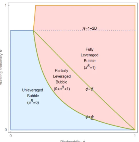
Figure 2: Existence regions
Several interesting comparative statics results arise from Propositions 1 and 2. First, we focus on parameter regions where bubbly equilibria exist. Figure 2 illustrates the regions
in the φ and π plane where unleveraged bubbly equilibria exist and where leveraged bubbly equilibria exist. These non-overlapping regions correspond to the set of parameters such that φ ď φ and Rnb ă 1 ´ π for the existence of the unleveraged bubbly equilibrium (Proposition
1), and for the set of parameters such that φ ą φ and Rnb ă φ ` p1 ´ φqp1 ´ πqD for the
existence of the leveraged bubbly equilibrium (Proposition 2). Figure 2 also shows how the existence region for the leveraged bubbly equilibrium consists of two sub-regions: the region above the curve φ “ φ that corresponds to the existence region for the fully leveraged bubbly equilibrium, and the region below the curve that corresponds to the existence region for the partially leveraged bubbly equilibrium (recall Remark 2).
Also as seen from the figure, for a fixed risk of bursting π, the leveraged bubbly equi-librium exists if and only if the pledgeability parameter φ is sufficiently large. Similarly, a larger φ is associated with a larger interval for π such that the leveraged bubbly equilibrium exists.
An interesting observation is that leveraged bubbles can be riskier than unleveraged ones. In particular, if π ą π ” 1 ´ Rnb, then there does not exist any unleveraged bubbly
equilibrium, but there can be a leveraged bubbly equilibrium as long as φ is sufficiently large. Intuitively, in the unleveraged equilibrium, the investors in the bubbly asset market internalize all the risk of the bubble, as the investment is financed by their own funds. On the other hand, in the leveraged equilibrium, the leveraged investors do not fully internalize all of the risk of the bubble, because their investment is financed with defaultable debt. We summarize the discussion above as follows:
Corollary 2 (Existence regions).
1. For each vector of exogenous parameters, a bubbly equilibrium, if it exists, is unique. If φ ď φ (low pledgeability), then the bubbly equilibrium is unleveraged (aB “ 0). If φ ą φ (high pledgeability), then the bubbly equilibrium is leveraged (aB
ą 0).
2. Leveraged bubbles tend to be riskier than unleveraged bubbles, in the sense that for each φ, any bubbly equilibrium where the risk of bursting π exceeds π ” 1 ´ Rnb “ 1 ´ 2D
must be leveraged.
Proof. Immediate corollary of Propositions 1 and 2.
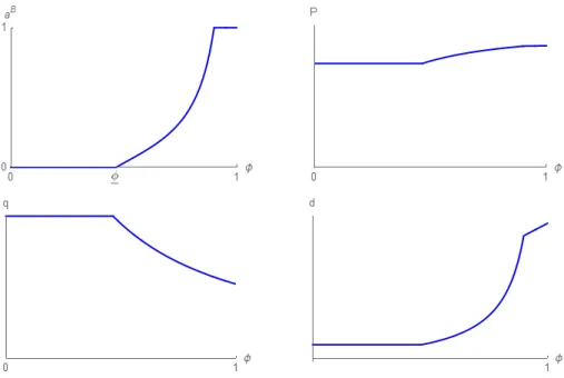
Going beyond existence conditions, Figure 3 provides numerical comparative statics of equilibrium prices and quantities in the bubbly equilibrium when the pledgeability parameter φ is allowed to vary. We set parameter values for π and D such that a bubbly equilibrium always exists for any φ P r0, 1s.9 Recall from Corollary 2 that the bubbly equilibrium is
9In particular, we set parameters so that R
Figure 3: Equilibrium quantities and prices as functions of φ
unique, allowing us to plot endogenous variables aB, P , q, and d in the stationary equilibrium as functions of the exogenous parameter φ.
As seen in the first panel, when φ is small, the bubbly equilibrium is unleveraged (aB “ 0), but when φ is large, the bubbly equilibrium becomes leveraged (aB
ą 0), and in general the bubbly asset position of the representative borrower aB is weakly increasing in φ. The
borrowers’ higher demand for the bubbly asset at higher φ is associated with a higher price of the bubbly asset, a higher level of debt, and a lower price of debt (or equivalently, a higher face-value interest rate). As the figure shows, P and d are weakly increasing and q is weakly decreasing in φ.10
6
Discussion and extensions
6.1
Individual-specific debt pricing
We have shown the main result that equilibria with risky leveraged bubbles can emerge when individual debt contracts are pooled. In this section, we show how this result crucially depends on the assumption of the credit pool.
Recall that under pooling, the market price of debt q (or equivalently the interest rate 1{q) only reflects the aggregated default risk across all borrowers. Now, we remove this
10When φ ă φ, the bubbly equilibrium is unleveraged, and a change in φ has no effect on equilibrium
assumption and instead assume that when an individual borrower i issues dB,i units of debt that are backed by ai units of the bubbly asset, she faces a price of debt qpdB,i, aB,i
q (or equivalently an interest rate 1{qpdB,i, aB,i
q) that reflects the individual default risk of this agent, as in the case of a bilateral loan contract between a bank and a borrower.11 The
competitive price of debt is given by:
qpdB,i, aB,iq “ $ & % qrf ” p1 ´ πqΛ h` πΛl if 0 ď dB,i ď D
p1 ´ πqΛh` πΛldDB,i if D ă dB,i ď D ` φP aB,i
, (31)
where Λh and Λl are the stochastic discount factors of the lenders in equilibrium. In the first
case, debt is fully backed by the fundamental collateral and there is no risk of default; hence the price of debt is given by the risk-free price qrf. In the second case, debt is backed by the bubbly collateral and there will be default when the bubble collapses; hence the price of debt is given by p1 ´ πqΛh` πΛldDB,i, where D{d
B,i is the recovery rate in the case of default. We
continue to impose the assumption that the promised repayment is bound by the maximum value of the collateral asset plus recourse: dB,i
ď D ` φP ai.
The definition of an equilibrium is similar to before, except that the price of debt is given by the expression above, and the optimization of the representative borrower takes into account the effects of her choice of debt and asset holding on the price of debt:
max
aB,it ě0,dB,it ě0
ErU pcB,i0,t, cB,i1,t`1qs,
subject to: cB,i0,t ` ξtPta B,i t “ qtpd B,i t , a B,i t qd B,i t
cB,i1,t`1 “ 1 ` ξt`1Pt`1aB,it ´ mintdit, D ` φξt`1Pt`1aB,it u
dit ď D ` φPt`1aB,it .
We will show that under this setup, the leveraged bubbly equilibrium will not exist except when φ “ 1 (maximum pledgeability). When φ “ 1, the leveraged bubbly equilibrium is payoff equivalent to the unleveraged bubbly equilibrium.12
Proposition 3 (No credit pool).
11This pricing of debt is also similar the pricing of debt issued by governments in the sovereign debt
literature.
12This result is related to Fostel and Geanakoplos (2015), who find that in a similar environment where
1. Suppose φ ă 1. Then there is a unique bubbly equilibrium. This equilibrium is unlever-aged, as borrowers do not buy the bubbly asset (aB
“ 0).
2. Suppose φ “ 1. Then there exist two bubbly equilibria: an unleveraged equilibrium where aB
“ 0, and a leveraged equilibrium where aB “ 1. The two equilibria are payoff equivalent, i.e., they yield the same consumption profiles for borrowers and savers. Proof. Appendix A.4.
In other words, this result shows that the existence of the leveraged bubbly equilibrium crucially depends on the assumption of the credit pool. Without the credit pool, the price of debt reflects the default risk of each individual borrower’s portfolio. This effectively rules out the incentive for borrowers to undertake the leveraged investment strategy.
Similarly, our leveraged bubbly equilibrium results would not arise under a richer asset market structure allowing for multiple credit pools with different credit limits. Intuitively, multiple credit pools would allow a sorting of borrowers similar to that induced by the bilateral loan contracts analyzed in this section, thus eliminating the under-pricing of safe debt characteristic of our single credit pool framework. This suggests that the pooling of different types of credit risks is important for the existence of leveraged bubbles.
6.2
Extensions
6.2.1 Lenders can default
So far, we have assumed that lenders can perfectly commit to not defaulting. We relax this assumption in this section and show that as long as the savings of lenders can be seized in the case of default, then it is never optimal for lenders to default in equilibrium. Intuitively, unlike borrowers, lenders have high endowment when young but low endowment when old, and thus they have a high marginal utility of consumption in old age. Should a lender default in the bad state, as her savings will be seized, the consumption would be very low, generating a very low utility.
Formally, we assume that in the case where lenders default, a fraction φs of their savings
(in addition to a fraction φ of their bubbly asset holdings and a fraction D of their old age income) can be garnished. Below, we show that as long as φs is sufficiently high, lenders
will not have an incentive to default in any equilibrium. In particular, if we set φs “ 1, then
lenders would never want to default.
Taking prices as given, each young lender chooses a portfolio consisting of a units of the bubbly asset, l shares of the credit pool (savings), and d units of debt issuance into the credit pool (borrowing). Her borrowing is subject to the following credit limit: d ď φP a ` φsl. Let
∆l denote the recovery in the bad state when the bubble collapses.13 Then the associated
consumption profile is given by:
cL0 “ 1 ` qd ´ pP a ` qlq cL1,h “ P a ` l ´ d
cL1,l “ ∆l¨ l ´ mintd, φs∆l¨ lu
Consider the option of defaulting in the bad state for a lender. Her consumption in that state would be cL
1,l “ p1 ´ φsq∆l¨ l. Thus, a higher pledgeability of savings φs would mean
a lower consumption in the bad state. A sufficiently high φs would substantially lower the
period utility lnpcL
1,lq. In particular, if we set φs “ 1, then the lender would never want to
default, as the utility function severely punishes a zero consumption level.14
It is then straightforward to show that, given lenders’ endowment path and without the incentive to default, lenders would choose their borrowing to be zero. Hence, their optimization problem effectively reduces to the optimization problem (5) as described in the main text.
6.2.2 Bubble attached to asset with fundamental value
In the main model, we have assumed for simplicity that the bubbly asset does not pay any dividend. It is straightforward to extend the model to allow for a bubbly asset that is attached to an asset with a fundamental value. We have in mind the case of a bubble attached to a housing asset, which yields utility dividend. Our approach of modeling the bubble attached to an asset with a fundamental value is similar to the standard approach developed by Blanchard and Watson (1982). We acknowledge that while this approach is tractable and appropriate for our analysis, it abstracts away from other important aspects of housing bubbles, such as the distortions in factor allocations resulting from the construction of additional dwellings during a housing bubble episode.
We continue to assume that there is a fixed unit supply of a perfectly divisible housing asset. Each agent i derives additive utility from owning ai units of the asset: the agent’s
utility over consumption and asset holding is U pci0, ci1q`vpaiq, where for simplicity we assume
that v is a linear utility function. Appendix B.1 provides the derivations of the unleveraged and leveraged bubbly equilibria, in a similar manner to that in Sections 4 and 5. As in the main Propositions 1 and 2, it also derives the main implication that the bubbly equilibrium
13The recovery rate is 1 in the good state when the bubble persists, as under the credit limit above, it is
never optimal for lenders to default in the good state.
14More generally, the argument applies for φ
is unleveraged if the pledgeability parameter φ is low and is leveraged if it is high. 6.2.3 Investment
We have focused so far on an endowment economy. However, our main result about how the credit pool facilitates leveraged bubbles applies to environments with investment as well. In this section, we provide a simple modification of the current model to allow for investment. The endowment profiles are as in the main model. However, assume for simplicity that agents consume only in old age and are risk neutral. When young, agents can invest in a production function f pkq. For tractability, we assume f pkq ” Akpζ ´ kq, where A is a constant TFP term and ζ ą 2 is a constant. It is immediate that f is strictly increasing and strictly concave for k P r0, 1s.
Instead of problem (4), the optimization problem of a representative borrower is given by:
max
aB tě0,dtě0
EtrcBt`1s
subject to budget constraints:
ktB` ξtPtaBt “ qtdt
cBt`1 “ 1 ` ξt`1Pt`1atB´ mintdt, D ` φξt`1Pt`1aBt u
and subject to the credit limit (3): dtď D ` φPt`1aBt .
And instead of problem (5), the optimization problem of a representative lender is: max
aL tě0,ltě0
EtrcLt`1s
subject to budget constraints:
ktL` ξtPtaLt ` qtlt “ 1
cLt`1 “ ξt`1Pt`1aLt ` ˜∆t`1lt,
where the delivery rate in equilibrium is given by (2).
Appendix B.2 provides (analytical) solutions to the model. It also shows that in the unleveraged bubbly equilibrium, the bubble crowds out aggregate output, as some resources are diverted away from productive investment and into bubble speculation. This is similar to the crowd-out effect in standard rational bubble models à la Tirole (1985). On the other hand, in the leveraged bubbly equilibrium, the bubble also has a crowd-in effect. This is because the pledgeable bubbly asset allows borrowers to increase their borrowing and
hence crowd-in their productive investment. This is similar to the crowd-in effect of bubbles in recent models (see, e.g., Miao and Wang, 2012; Martin and Ventura, 2012; Hirano and Yanagawa, 2016). There are parameter conditions under which the crowd-in effect dominates the crowd-out effect. In this sense, among the two types of bubbly equilibria that can arise in our model, the leveraged bubbly equilibrium appears to be more consistent with the stylized observation that most bubble episodes are associated with investment booms.
7
Conclusion
We have presented a simple tractable general equilibrium model of endogenously leveraged bubbles. The theory predicts that a high pledgeability of bubbly assets and the packaging of debt into a competitive credit pool facilitates leveraged bubble episodes. In a leveraged bubble episode, borrowers finance their purchase of risky bubbly assets with collateralized loans from savers. When a leveraged bubble bursts, borrowers find themselves “underwater” and optimally choose to default. Throughout history, the collapses of leveraged bubbles, such as those experienced by Japan in the 1990s and the U.S. in the 2000s, have often been associated with default and crises (e.g., Kindleberger and Aliber, 2005; Jordà et al., 2015). The model presented in this paper provides a tractable framework in which the precursors and consequences of such leveraged bubble episodes can be analyzed.
Acknowledgements
We thank Xavier Vives (editor), an anonymous associate editor, two anonymous referees, as well as David Andolfatto, Vladimir Asriyan, Kartik Athreya, Roland Bénabou, Matthias Doepke, Oded Galor, Lutz Hendricks, Anton Korinek, Kiminori Matsuyama, Alberto Martin, Pietro Peretto, Gilles Saint-Paul, Juan Sanchez, Jaume Ventura, Fabrizio Zilibotti, and con-ference/seminar participants at Amherst College, Barcelona Summer Forum, Duke’s TDM workshop, FRB of St. Louis, FRB of Richmond, IMF, Kobe University, McGill, NBER EFBGZ, RIDGE, UNC, Université de Montréal, and University of Washington in Seattle for helpful comments and suggestions. Bengui is grateful to the Social Sciences and Humanities Research Council of Canada for funding this research under grant 430-2013-000250. Phan ac-knowledges the partial funding by Vietnam National Foundation for Science and Technology Development (NAFOSTED) under grant number 502.01-2017.12. This paper previously cir-culated under the title “Inequality, Financial Frictions, and Leveraged Bubbles.” The views expressed herein are those of the authors and not necessarily those of the Federal Reserve Bank of Richmond or the Federal Reserve System.
References
Abreu, D. and Brunnermeier, M. K. (2003). Bubbles and crashes. Econometrica, 71(1):173– 204.
Aiyagari, S. R. (1994). Uninsured idiosyncratic risk and aggregate saving. Quarterly Journal of Economics, 109(3):659–684.
Aiyagari, S. R. and Gertler, M. (1999). “overreaction” of asset prices in general equilibrium. Review of Economic Dynamics, 2(1):3–35.
Allen, F. and Gale, D. (2000). Bubbles and crises. The Economic Journal, 110(460):236–255. Allen, F. and Gorton, G. (1993). Churning bubbles. The Review of Economic Studies,
60(4):813–836.
Aoki, K. and Nikolov, K. (2015). Bubbles, banks and financial stability. Journal of Monetary Economics, 74:33–51.
Arce, Ó. and López-Salido, D. (2011). Housing bubbles. American Economic Journal: Macroeconomics, 3(1):212–241.
Barlevy, G. (2012). Rethinking theoretical models of bubbles. New Perspectives on Asset Price Bubbles.
Barlevy, G. (2014). A leverage-based model of speculative bubbles. Journal of Economic Theory, 153:459–505.
Barlevy, G. and Fisher, J. (2011). Mortgage choices and housing speculation. Technical report, Federal Reserve Bank of Chicago Working Paper.
Basco, S. (2016). Switching bubbles: From outside to inside bubbles. European Economic Review, 87:236–255.
Bernanke, B. and Gertler, M. (1989). Agency costs, net worth, and business fluctuations. The American Economic Review, 79(1):14–31.
Bewley, T. (1977). The permanent income hypothesis: A theoretical formulation. Journal of Economic Theory, 16(2):252–292.
Blanchard, O. J. and Watson, M. W. (1982). Bubbles, rational expectations and financial markets.
Boz, E. and Mendoza, E. G. (2014). Financial innovation, the discovery of risk, and the U.S. credit crisis. Journal of Monetary Economics, 62:1–22.
Caballero, R. J. and Farhi, E. (2015). The safety trap. Working Paper.
Cipriani, M., Fostel, A., and Houser, D. (2012). Leverage and asset prices: An experiment. Working paper.
Connor, G., Flavin, T., and O’Kelly, B. (2012). The US and Irish credit crises: Their distinctive differences and common features. Journal of International Money and Finance, 31(1):60–79.
Cooper, D. (2009). Impending U.S. spending bust? The role of housing wealth as borrowing collateral. Federal Reserve Bank of Boston Public Policy Discussion Paper, 9(9).
Diamond, P. A. (1965). National debt in a neoclassical growth model. The American Economic Review, 55(5):1126–1150.
Doblas-Madrid, A. and Lansing, K. (2014). Credit-fuelled bubbles. Working paper.
Dubey, P. and Geanakoplos, J. (2002). Competitive pooling: Rothschild-Stiglitz reconsid-ered. The Quarterly Journal of Economics, 117(4):1529–1570.
Dubey, P., Geanakoplos, J., and Shubik, M. (2005). Default and punishment in general equilibrium. Econometrica, 73(1):1–37.
Farhi, E. and Tirole, J. (2012). Bubbly liquidity. The Review of Economic Studies, 79(2):678– 706.
Fostel, A. and Geanakoplos, J. (2012). Tranching, CDS, and asset prices: How financial innovation can cause bubbles and crashes. American Economic Journal: Macroeconomics, 4(1):190–225.
Fostel, A. and Geanakoplos, J. (2015). Leverage and default in binomial economies: a complete characterization. Econometrica, 83(6):2191–2229.
Geanakoplos, J. (1997). Promises, promises. In Arthur, W., Durlauf, S., and Lane, D., editors, The Economy as an Evolving Complex System, II, pages 285–320. Addison-Wesley. Geanakoplos, J. (2010). The leverage cycle. In NBER Macroeconomics Annual 2009,
Geanakoplos, J. and Zame, W. R. (2002). Collateral and the enforcement of intertemporal contracts. Cowls Foundation Working Paper.
Geanakoplos, J. and Zame, W. R. (2014). Collateral equilibrium, I: A basic framework. Economic Theory, 56(3):443–492.
Ghent, A. C. and Kudlyak, M. (2011). Recourse and residential mortgage default: evidence from us states. The Review of Financial Studies, 24(9):3139–3186.
Greenspan, A. (2013). Bubbles and leverage cause crises: Alan Greenspan; CNBC interview with Matthew Belvedere. http://www.cnbc.com/id/101135835. Accessed: 2017-10-18. Herring, R. J. and Wachter, S. (1999). Real estate booms and banking busts: An
interna-tional perspective. Technical report, Wharton School Center for Financial Institutions, University of Pennsylvania.
Hirano, T., Inaba, M., and Yanagawa, N. (2015). Asset bubbles and bailouts. Journal of Monetary Economics, 76:S71–S89.
Hirano, T. and Yanagawa, N. (2016). Asset bubbles, endogenous growth, and financial frictions. The Review of Economic Studies, 84(1):406–443.
Huggett, M. (1993). The risk-free rate in heterogeneous-agent incomplete-insurance economies. Journal of Economic Dynamics and Controls, 17:953–969.
Hunter, W. C., Kaufman, G. G., and Pomerleano, M. (2005). Asset price bubbles: The implications for monetary, regulatory, and international policies. MIT press.
Ikeda, D. and Phan, T. (2016). Toxic asset bubbles. Economic Theory, 61(2):241–271. Jordà, Ò., Schularick, M., and Taylor, A. M. (2015). Leveraged bubbles. Journal of Monetary
Economics, 76:S1–S20.
Kelly, M. (2009). The Irish credit bubble. Journal of Finance, 61(5):2511–2546.
Kindleberger, C. and Aliber, R. (2005). Manias, Panics, and Crashes: A History of Financial Crises, 5th edition. Hoboken, NJ: John Wiley & Sons.
Kiyotaki, N. and Moore, J. (1997). Credit cycles. The Journal of Political Economy, 105(2):211–248.
Kocherlakota, N. (2009). Bursting bubbles: Consequences and cures. Unpublished manuscript, Federal Reserve Bank of Minneapolis.
Martin, A. and Ventura, J. (2012). Economic growth with bubbles. American Economic Review, 102(6):3033–3058.
Martin, A. and Ventura, J. (2016). Managing credit bubbles. Journal of the European Economic Association, 14:753–789.
Martin, A. and Ventura, J. (2017). The macroeconomics of rational bubbles: a user’s guide. Working paper.
Mian, A. and Sufi, A. (2009). The consequences of mortgage credit expansion: Evidence from the U.S. mortgage default crisis. The Quarterly Journal of Economics, 124(4):1449–1496. Mian, A. and Sufi, A. (2011). House prices, home equity–based borrowing, and the U.S.
household leverage crisis. The American Economic Review, 101(5):2132–2156.
Mian, A. and Sufi, A. (2014). House of Debt: How They (and You) Caused the Great Recession, and How We Can Prevent It from Happening Again. University of Chicago Press.
Miao, J. (2014). Introduction to economic theory of bubbles. Journal of Mathematical Economics, 53:130–136.
Miao, J. and Wang, P. (2011). Bubbles and credit constraints. Working Paper.
Miao, J. and Wang, P. (2012). Bubbles and total factor productivity. American Economic Review, Papers and Proceedings, 102(3):82–87.
Miao, J. and Wang, P. (2015). Banking bubbles and financial crises. Journal of Economic Theory, 157:763–792.
Miao, J., Wang, P., and Zhou, J. (2014). Housing bubbles and policy analysis. Working Paper.
Mishkin, F. (2009). Not all bubbles present a risk to the economy. Financial Times, 9. Mishkin, F. S. (2008). How should we respond to asset price bubbles? Banque de France,
Financial Stability Review, 12:65–74.
Rajan, R. G. (2011). Fault Lines: How hidden fractures still threaten the world economy. Princeton University Press.
Samuelson, P. A. (1958). An exact consumption-loan model of interest with or without the social contrivance of money. The Journal of Political Economy, 66(6):467–482.
Shioji, E. (2013). The bubble burst and stagnation of Japan. Routledge Handbook of Major Events in Economic History, page 316.
Simsek, A. (2013). Belief disagreements and collateral constraints. Econometrica, 81(1):1–53. Tirole, J. (1985). Asset bubbles and overlapping generations. Econometrica, 53(6):1499–
1528.
Weil, P. (1987). Confidence and the real value of money in an overlapping generations economy. The Quarterly Journal of Economics, 102(1):1–22.
Zhao, B. (2015). Rational housing bubble. Economic Theory, 60(1):141–201.
A
Appendix: Proofs
A.1
Proof of Proposition 1
We start by proving the first claim. An unleveraged bubbly equilibrium by definition requires aB
“ 0 and aL “ 1 (equation (8)). Since borrowers do not hold the bubbly asset, the security pool is safe and the delivery rate is equal to 1 regardless of the state. Borrowers’ credit constraint d ď D must bind, for if it did not, their unconstrained Euler equation for borrowing would require d ě 1{2 ą D. Equilibrium borrowing and lending must thus be given by d “ D and l “ ´D (equation (9)). Given the portfolio positions, equilibrium consumption must be given by the expressions in (11) and (10). Since lenders are the marginal buyers of both the security and the bubbly asset, their Euler equations (12) and (13) have to hold with equality. It is then straightforward to verify that with upcq “ lnpcq, the system of equations (12)-(13) admits the unique solution provided in (14)-(15).
We now turn to the second claim. From the uniqueness derived in the first claim, it follows that an unleveraged bubbly equilibrium exists if and only if the specified allocations and prices constitute an equilibrium. This is the case if and only if two conditions are satisfied.
First, by definition, the bubbly asset price must be positive, i.e., PU ą 0. From (14),
that this is the case if and only if D ă 1´π2 , i.e., condition (18).
Second, for the conjectured equilibrium to be valid, it must be that there exists no profitable deviation for agents. There is by construction no profitable deviation for lenders, since lenders’ optimality conditions are satisfied at the conjectured equilibrium. We therefore
derive a condition such that there is no profitable deviation for borrowers either. A borrower’s equilibrium payoff is given by
vB “ upqUDq ` up1 ´ Dq.
Meanwhile, a borrower’s deviation payoff is given by ˆ vBpφq ” max ˆ aě0, ˆdďD`φPUaˆ u ´ qUd ´ Pˆ Uˆa ¯ ` p1 ´ πqu ´ 1 ` PUˆa ´ ˆd ¯ ` πu ´ 1 ´ mint ˆd, Du ¯ .
We now proceed to show that we can assume without loss of generality that the borrower’s credit constraint binds at an optimum, i.e., that ˆd “ D ` φPUˆa. To this end, we consider
two related sub-problems. In the first sub-problem, we constrain a borrower to issue debt in the safe region (0 ď ˆd ď D). In the second sub-problem, we constrain a borrower to issue debt in the risky region (D ď ˆd ď D ` φPUˆa). In the first case, we will argue that the
optimal choice is ˆa “ 0 and ˆd “ D, which coincides with the conjectured equilibrium choice and hence does not give rise to a profitable deviation. In the second case, we will argue that the optimal choice necessarily features ˆd “ D ` φPUˆa.
The first sub-problem is given by: max ˆ aě0, ˆdďD u ´ qUd ´ Pˆ Uˆa ¯ ` p1 ´ πqu ´ 1 ` PUa ´ ˆˆ d ¯ ` πu ´ 1 ´ ˆd ¯ .
The FOCs, which are necessary and sufficient for an optimum, are given by 1
qUd ´ Pˆ Uˆa
ě p1 ´ πq 1 1 ` PUa ´ ˆˆ d
, (A.1)
where the condition holds with equality if ˆa ą 0, and by qU qUd ´ Pˆ Uˆa ě p1 ´ πq 1 1 ` PUˆa ´ ˆd ` π 1 1 ´ ˆd, (A.2) where the condition holds with equality if ˆd ă D. To show that an optimum necessarily requires ˆa “ 0, suppose instead that ˆa ą 0, seeking a contradiction. In this case, the borrower’s Euler equation for the bubbly asset in (A.1) must hold with equality, which
requires15 ˆ a “ r1 ` p1 ´ πq qUs ˆd ´ 1 r1 ` p1 ´ πqs PU ď “1 ` p1 ´ πq `1 ` π 2D˘‰ D ´ 1 r1 ` p1 ´ πqs PU ď D ` 1 2 `1 2 ` D ˘2 ´ 1 r1 ` p1 ´ πqs PU ă 0,
a contradiction. It follows that ˆa “ 0. Next, to show that an optimum requires ˆd “ D, suppose instead that ˆd ă D, seeking a contradiction. In this case, the borrower’s Euler equation for the debt security in (A.2) must hold with equality, which requires ˆd “ 1{2, a contradiction with the credit constraint ˆd ď D ă 1{2. It follows that ˆd “ D. Hence, the solution to the first sub-problem is ˆa “ 0 and ˆd “ D, which coincides with the conjectured equilibrium choice and thus does not give rise to a profitable deviation.
The second sub-problem is given by: max ˆ aě0,Dď ˆdďD`φPUˆa u ´ qUd ´ Pˆ Uˆa ¯ ` p1 ´ πqu ´ 1 ` PUa ´ ˆˆ d ¯ ` πu p1 ´ Dq .
The FOCs, which are necessary and sufficient for an optimum, are given by: 1
qUd ´ Pˆ Uˆa
ě p1 ´ πq 1 1 ` PUa ´ ˆˆ d
,
where the condition holds with equality if ˆa ą 0, and by: qU
qUd ´ Pˆ Uˆa
£ p1 ´ πq 1 1 ` PUa ´ ˆˆ d
,
where the condition holds with ď if ˆd “ D, with “ if D ă ˆd ă D ` φPUa, and with ě ifˆ
ˆ
d “ D ` φPUˆa. To show that an optimum necessarily requires ˆa “ D ` φPUˆa, we observe
that qU qUd ´ Pˆ Uˆa ą 1 qUd ´ Pˆ Uˆa ě p1 ´ πq 1 1 ` PUˆa ´ ˆd (A.3) where the first inequality follows from the fact that qU ą 1. Therefore, a borrower’s deviation
15To establish the second inequality, we note that the numerator of the expression in the second line is