Science Arts & Métiers (SAM)
is an open access repository that collects the work of Arts et Métiers Institute of
Technology researchers and makes it freely available over the web where possible.
This is an author-deposited version published in:
https://sam.ensam.eu
Handle ID: .
http://hdl.handle.net/10985/19580
To cite this version :
Faissal CHEGDANI, Mohamed EL MANSORI, Amen-Allah CHEBBI - Numerical modeling of
micro-friction and fiber orientation effects on the machinability of green composites - Tribology
International - Vol. 150, p.106380 - 2020
https://doi.org/10.1016/j.triboint.2020.106380
Finite element modeling Machining
Microscale friction
and the components of the composite structure. A 2D micromechanical model for orthogonal cutting of flax fibers reinforced polylactic-acid (PLA) composites is considered in this study at different orientation of fibers. Results show that the numerical thrust forces are significantly affected by the variation of the micro-friction in the model. An optimized value of the micro-friction coefficient has been found to fit with the experimental results. The FE model provides the ability to calculate with good accuracy the effect of fiber orientation on the machinability of flax/PLA composites.
1. Introduction
Natural fiber reinforced polymer (NFRP) composites are nowadays used in different industrial sectors thanks to many technical, economic, and ecological advantages comparing to glass fiber reinforced polymer (GFRP) composites [1,2]. NFRP composites mean polymer composites that are reinforced with natural fibers, especially plant fibers (flax, hemp, jute …). When the polymer matrix is also bio-based, the resulting NFRP composites can be called green composites. These kinds of eco-friendly materials are biodegradable and recyclable which contrib-utes to a circular economy and a sustainable development [3–5].
Machining operations on NFRP composites generate many issues related to the cutting behavior of plant fibers within the composite [6–9]. Indeed, due to the complex cellulosic structure of natural fibers based on cellulose microfibrils toward the fiber axis, plant fibers are characterized by a high transverse elasticity that favors the fibers deformation and, consequently, avoids an efficient fiber shearing during the cutting processes [10]. This makes the machining of NFRP com-posites highly sensitive to the process parameters. Moreover, the natural fibrous reinforcement is characterized by a multiscale structure starting from the microscopic scale of the elementary fibers, then the mesoscale of the fibers bundle (the technical fiber), and the macroscale of the composite structure [10]. This multiscale structure makes the machin-ability analysis of NFRP composites highly sensitive to the analysis scale,
typically for the investigation of the machined surfaces [10]. To resolve this issue, a new multiscale approach has been developed for the ex-amination of the machinability of the NFRP composites. This approach postulates that the machinability analysis of NFRP composites requires the selection of the relevant scale which corresponds to the size of the natural fibrous reinforcement [11]. Therefore, before starting the anal-ysis of the machined surfaces of NFRP composites, the natural fibrous reinforcement should be analyzed to measure the size of the considered fibrous structure (elementary fibers, technical fibers, fiber yarns …). The topographic image size should correspond to the considered fibrous structure size in order to get an efficient discrimination of the effects of the different process parameters.
The new multiscale approach has shown its effectiveness on the machinability analysis of NFRP composites through an industrial application [11]. However, its application still encounters some limi-tations. Indeed, it is well known that the size of the natural fiber rein-forcement shows a high variability due to the random size and shape of natural fibers within the same bundle [12], which is due to some envi-ronmental factors (pluviometry and sunshine) and mechanical factors of the extraction processes. Therefore, for the same fibers type that are grown in the same location, the relevant scale could be different from one harvest to another since the fibrous structure size may vary signif-icantly. For these reasons, the multiscale approach should be re-applied to each fibers harvest, which is time and cost consuming.
* Corresponding author.
To avoid this issue, developing a numerical model for machining of NFRP composites could reduce considerably the time and the cost of the machinability analysis during the experimental validation of new NFRP composite products. For this aim, the authors have developed in a pre-vious work a 2D finite element model at microscale to simulate the orthogonal cutting behavior of natural flax fibers reinforced poly-propylene composites [13]. Unlike synthetic fibers (glass and carbon), flax fibers were modeled using an elastoplastic law and a ductile damage criterion. The finite element (FE) micromechanical model can reproduce qualitatively the cutting behavior of natural fibers during the machining operation at different cutting speed values. Quantitatively, the cutting forces are well reproduced by the FE model in terms of trend and magnitude. For the thrust forces, the trends are well reproduced by the FE model but there is a factor of ~3 for magnitude between FE results and experimental outputs [13]. The same phenomenon has been observed for the FE modeling of the machining of synthetic fiber com-posites [14,15]. The magnitude difference in thrust force results be-tween the FE model and the experiments has been explained by the fibers spring back that is not considered in the numerical model. Nevertheless, no theoretical or experimental evidence can confirm this hypothesis.
A different approach is investigated in this paper to address the issue of the thrust force correlation in the FE modeling of NFRP machining. This approach is based on the machining tribology, especially the micro- friction between the composite and the cutting tool. The micro-friction means the local friction between the cutting tool and each composite phase component at microscale (elementary natural fibers and polymer matrix). The considered investigation is motivated by previous authors works on the local micro-friction on NFRP composites by scratch-test
experiments [16,17]. Indeed, the first scratch-test experiments were done with a diamond Berkovich tip indenter and the friction coefficient has been found around 0.4 for polypropylene (PP) matrix and around 0.5 for flax fibers [16]. These values were used in the previous FE model of machining [13]. However, the following scratch-test experiments were done with a Sapphire Berkovich tip indenter and the friction co-efficient has been found around 0.2 for both PP matrix and flax fibers at the same scratching conditions as the experiments with the diamond indenter [17]. This indicates that the tool material causes a significant modification of the frictional properties in the case of NFRP composites. Therefore, the values of the micro-friction used in the previous FE machining model may be not appropriate because the experimental machining tests were performed by a carbide cutting insert. This could be the origin of the magnitude difference in the thrust forces of the FE machining model.
In this paper, the FE micromechanical model for machining of NFRP composites is used to investigate the effect of the micro-friction on the machining forces at different values of fiber orientation. A green com-posite is considered in this study and it is composed of flax fibers embedded in a natural polymer matrix of polylactic-acid (PLA). More-over, the FE cutting behavior of flax fibers is compared to that observed with scanning electron microscope (SEM) on the experimental machined surfaces for each fiber orientation.
2. Finite element modeling
2.1. Geometrical setup
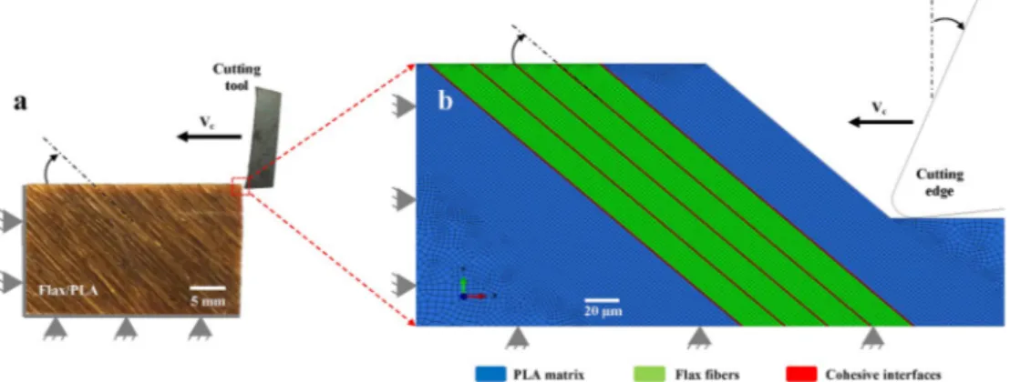
The FE model developed in Ref. [13] has been considered in this Fig. 1. (a) Image of the orthogonal cutting configuration at the real experimental scale. (b) Image of the 2D micromechanical cutting model showing the three
composite components and the fiber orientation.
study to investigate the effect of the micro-friction between the cutting tool and each component of the composite. FE simulations are carried out using ABAQUS/Explicit software (version 6.11-2) [18]. Fig. 1 shows the transition from the real macroscopic scale of the experimental orthogonal cutting operation (Fig. 1(a)) to the finite element model developed at microscale with consideration of the fiber orientation (Fig. 1(b)).
The microscopic-based model consists of a bundle of four elementary flax fibers embedded in a natural polymer of polylactic-acid (PLA). As shown in Fig. 1(b), the interfaces between fibers and matrix are modeled with cohesive elements that have a thickness of 1 μm. Each elementary fiber has a diameter of 15 μm. The cutting tool is considered as an analytical rigid body where the movement is controlled by a reference point. Flax fibers are oriented with an angle “θ” from the cutting di-rection. A plane stress analysis, which is more suitable for FEM cutting of composites [15], is considered in this numerical investigation. Both flax fibers and PP matrix are meshed with 4-node bilinear plane stress quadrilateral elements (CPS4R) and 2 μm of mesh size. Cohesive in-terfaces are meshed with a 4-node two-dimensional cohesive element (COH2D4) and 1 μm of mesh size.
As for synthetic fiber composites, the thermal effect is not considered in this micromechanical study because the heat generation in orthogonal cutting requires a large cutting length [19,20]. The cutting length in the current model does not exceed 200 μm.
In the present model, five fiber orientations are considered (θ ¼ 0�, θ
¼25�, θ ¼ 45�, θ ¼ 65�, and θ ¼ 90�) as shown in Fig. 2. Only the positive
fiber orientations range (from 0�to 90�with respect to the cutting
di-rection) is considered because the negative fiber orientations range (from 90� to 180� with respect to cutting direction) lead to poor
machinability of composites with a high delamination rate due to the torn-off of fibers [21].
For θ ¼ 0�, the cutting edge is considered to be firstly in contact with
the matrix before getting into contact with the cross-section of an elementary flax fiber (Fig. 2(a)) and the removed material across the cutting depth is supposed to contain a bundle of three elementary flax fibers embedded in the PLA matrix.
2.2. Micromechanical modeling
Unlike synthetic fibers such as glass or carbon, the cellulosic struc-ture of natural plant fibers generates an elastoplastic behavior that is due to the rearrangement of cellulosic microfibrils toward the fiber axis [22–25] as shown in Fig. 3(a). The PLA matrix generates an elastoplastic behavior [26] that is well-known for the thermoplastic polymers as shown in Fig. 3(b).
The cellulosic structure of natural plant fibers gives them an aniso-tropic behavior where the privileged direction is toward the fiber axis. The behavior of PLA is assumed isotropic. The considered values of elastic properties of both flax fibers and PLA are presented in Table 1. It’s important to notice that the mechanical properties of flax fibers show a high variability [27]. Therefore, the mechanical inputs of Table 1
are chosen to be as closer as possible to those of flax fibers used in the experimental validation.
The longitudinal plastic behavior of flax fibers is implemented using 30 points on the yield stress versus plastic strain curve from Fig. 3(a) with a maximum yield stress of 750 MPa. For the PLA, the plastic behavior is also implemented using 20 points on the yield stress versus strain curve from Fig. 3(b).
To model the anisotropic plasticity-based failure for flax fibers, the Hill’s potential function is used [28]. Hill’s potential function is a simple extension of the Mises function, which can be expressed in terms of rectangular Cartesian stress components (σij) as following [18,29]: f ðσÞ¼
ffiffiffiffiffiffiffiffiffiffiffiffiffiffiffiffiffiffiffiffiffiffiffiffiffiffiffiffiffiffiffiffiffiffiffiffiffiffiffiffiffiffiffiffiffiffiffiffiffiffiffiffiffiffiffiffiffiffiffiffiffiffiffiffiffiffiffiffiffiffiffiffiffiffiffiffiffiffiffiffiffiffiffiffiffiffiffiffiffiffiffiffiffiffiffiffiffiffiffiffiffiffiffiffiffiffiffiffiffiffiffiffiffiffiffiffiffiffiffiffiffiffiffiffiffiffiffiffiffiffiffiffiffiffi Fðσ22 σ33Þ2þGðσ33 σ11Þ2þHðσ11 σ22Þ2þ2Lσ232 þ2Mσ231þ2Nσ212
q
(1) Where F, G, H, L, M and N are constants defined as following:
F ¼ðσ 0Þ2 2 � 1 σ2 22 þ 1 σ2 33 þ 1 σ2 11 � ¼1 2 � 1 R2 22 þ 1 R2 33 þ 1 R2 11 � (2) G ¼ðσ 0Þ2 2 � 1 σ2 33 þ 1 σ2 11 1 σ2 22 � ¼1 2 � 1 R2 33 þ 1 R2 11 1 R2 22 � (3)
Fig. 3. Typical stress/strain curves of (a) elementary flax fiber (adapted from Ref. [25]) and (b) PLA matrix (adapted from Ref. [26]).
Table 1
Main mechanical properties used in the FE model.
Material Property Direction Value Unit Reference
Flax fibers Stiffness E11 50 GPa [13,29]
E22 ¼E33 12 G12 ¼G13 ¼G23 3.4 Poisson ratio ν12 0.178 – ν13 ¼ν23 0.2 Strength S11 750 MPa S22 ¼S33 150 S12 ¼S13 ¼ S23 20 Fracture
energy Gf 132 KJ/ m2 Calculated from data of [13,29]
PLA matrix Stiffness E 1.4 GPa [26]
Poisson ratio ν 0.35 – Strength S 64 MPa Fracture energy Gf 5 KJ/ m2 Cohesive zone Stiffness Knn ¼Kss ¼ Ktt Kns ¼Knt ¼ Kst 38
0 GPa/ mm Calculated from data of [36]
Strength t0
n¼t0s ¼t0t 18 MPa [36,37]
Fracture
energy G
H ¼ðσ 0Þ2 2 � 1 σ2 11 þ 1 σ2 22 1 σ2 33 � ¼1 2 � 1 R2 11 þ 1 R2 22 1 R2 33 � (4) L ¼3 2 � τ0 σ23 �2 ¼ 3 2R2 23 (5) M ¼3 2 � τ0 σ13 �2 ¼ 3 2R2 13 (6) N ¼3 2 � τ0 σ12 �2 ¼ 3 2R2 12 (7) where each σij is the measured yield stress value when σij is applied as
the only nonzero stress component, τ0¼σ0ffiffi
3
p where σ0 is the reference
yield stress which is set to be equal to σ11in this case; Rij are anisotropic
yield stress ratios that are needed to implement the Hill’s potential function in the FE model [18] and are defined as follows where the considered strength values are provided in Table 1:
R11¼σ11 σ0 (8) R22¼σ22 σ0 (9) R33¼σ33 σ0 (10) R12¼σ12 τ0 (11) R13¼ σ13 τ0 (12) R23¼ σ23 τ0 (13)
A ductile criterion [30] is considered to model the failure of both flax fibers and PLA. The ductile criterion is based on a fracture diagram which gives the equivalent plastic strain at fracture as a function of the stress state. The model assumes that the equivalent plastic strain at the onset of damage is a function of stress triaxiality and strain rate. The criterion for damage initiation is met when the following condition is satisfied [30]: Z ε** eq 0 dεeq ε** eqðη; _ε plÞ¼1 (14)
where εeq is the equivalent plastic strain, ε**eq is the equivalent plastic
strain at fracture, _εpl is the equivalent plastic strain rate, and η is stress
triaxiality that can be calculated by the following equations [31]:
η¼σm
σeq (15)
Here σm denotes the hydrostatic stress and σeq is the Von Mises
equivalent stress that can be calculated by the following equations:
σm¼σ11 þσ22þσ33 3 (16) σeq¼ ffiffiffiffiffiffiffiffiffiffiffiffiffiffiffiffiffiffiffiffiffiffiffiffiffiffiffiffiffiffiffiffiffiffiffiffiffiffiffiffiffiffiffiffiffiffiffiffiffiffiffiffiffiffiffiffiffiffiffiffiffiffiffiffiffiffiffiffiffiffiffiffiffiffiffiffiffiffiffiffiffiffiffiffiffiffiffiffiffiffiffiffiffiffiffiffiffiffiffiffiffiffiffiffiffiffiffiffiffiffiffiffiffiffiffiffiffiffiffiffiffiffiffiffiffiffiffiffiffiffi 1 2½ðσ11 σ22Þ 2þ ðσ 22 σ33Þ2þ ðσ33 σ11Þ2þ6ðσ212þσ223þσ231Þ� r (17) As for the Hill’s potential function, the stress triaxiality criterion is calculated using the strength values of Table 1.
The damage evolution law describes the rate of degradation of the material stiffness once the corresponding initiation criterion has been reached. For elastoplastic materials, the damage evolution is carried out
in two forms: softening of the yield stress and degradation of the elas-ticity [18]. The damage evolution law can be specified either in terms of fracture energy per unit area (Gf) or the equivalent plastic displacement
(upl) which is related to the equivalent plastic strain (εpl) by the
following equation [32]: upl¼L
eεpl (18)
Leis a characteristic length related to the element. The definition of the
characteristic length depends on the element geometry and formulation: it is a typical length of a line across an element for a first-order element, and it is half of the same typical length for a second-order element [18]. The equivalent plastic displacement at failure is computed following the equation (19) where σy0is the value of the yield strength [18,32]. uplf ¼
2 Gf
σy0 (19)
In the FE model, the damage evolution is modeled using the fracture energy per unit area (Gf). This parameter is available in literature for
PLA. For flax fibers, the value used for Gfis estimated based on the
Griffith theory for ductile materials [33] using the equation (20) where
σf is the tensile strength, E is the Young modulus and a is the cracking
length that has been assumed to be equal to the elementary fiber diameter.
Gf¼
σ2
fπa
4E (20)
Interfaces are modeled using the cohesive zone model (CZM). The elastic behavior of the CZM is modeled using a linear elastic traction- separation behavior. It assumes initially linear elastic behavior fol-lowed by the initiation and evolution of damage. The elastic behavior is written in terms of an elastic constitutive matrix that relates the nominal stresses to the nominal strains across the interface following the equa-tion [18]: 8 < : tn ts tt 9 = ;¼ 2 4EEnnns EEnsss EEntst Ent Est Ett 3 5 8 < : εn εs εt 9 = ; (21)
Where tn, ts and tt are the nominal stresses in the normal, shear and
tangential directions, respectively. Eij are the components of the
elas-ticity matrix. εn, εs and εt are the nominal strains in the normal, shear and
tangential directions, respectively. The corresponding separations are denoted by δn, δs and δt and are defined as following, where T0 is the
initial thickness of the cohesive element [18]:
εn¼ δn T0 (22) εs¼ δs T0 (23) εt¼ δt T0 (24)
In Abaqus software, the penalty stiffness parameter (Kij) is
imple-mented to model the rigidity of the cohesive zone [34,35] and it is defined by the following equation:
8 < : tn ts tt 9 = ;¼ 2 4KKnnns KKnsss KKntst Knt Kst Ktt 3 5 8 < : δn δs δt 9 = ; (25)
Damage of cohesive zones is assumed to initiate when a quadratic interaction function involving the nominal stress ratios reaches a value of one. This criterion can be represented as following [18,29]: � htni t0 n �2 þ � ts t0 s �2 þ � tt t0 t �2 ¼1 (26)
t0
n, t0s and t0t are the peak values of the nominal stress components in the
normal, shear and tangential directions, respectively. The symbol 〈 〉 in the equation (26) represents the Macaulay bracket which is used to signify that a pure compressive deformation or stress state does not initiate damage [18].
2.3. Friction modeling
Friction is one of the most important phenomena that should be considered to model the machining operations. The significance of friction in machining is due to the high stresses and velocities generated during the tool-material contact. However, modeling friction in machining is a complicated task because it should consider different factors related to the contact geometry, especially the geometrical pa-rameters of the cutting tool edge such as the rake angle, the clearance angle and the cutting edge radius.
In metal cutting, it is usual to consider the tool as infinitely sharp, so the tool-material contact is along a perfect straight rake face [38]. Ac-cording to that assumption, and if the tool has not been subjected to wear (fresh tool), the whole pressure at the cutting contact has a con-stant direction and can be summed up in one resultant force in the same direction. Therefore, the cutting friction coefficient is constant along the tool face and can be calculated using the following equation derived from Merchant model [38].
μ¼FtþFctanðγÞ
Fc FttanðγÞ (27)
Where Fc is the cutting force (in the feed direction), Ft is the thrust force
(normal to the feed direction), and γ is the rake angle of the tool. If the process parameters (cutting speed and depth) are kept constant, the
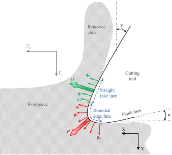
friction coefficient will depend highly on the rake angle of the tool. Nevertheless, the fact that the cutting tools have a rounded edge cannot be ignored for machining of fiber composites because this geometrical parameter has a significant impact of the cutting behavior of fibers [10,39,40], especially when machining natural fiber compos-ites that are highly sensitive to the small variations of the cutting edge radius [10]. In the following, the cutting friction is discussed by considering the rounded cutting edge.
As illustrated in Fig. 4, when considering a fresh tool with a rounded edge, two contact regions can be defined. The first contact region is between the removed chip and the straight rake face. The tool-material contact in this region is similar to that described with Merchant model [38]. The resultant contact force (Q in Fig. 4) is obtained by summing the infinitesimal forces along the straight rake face (q1, q2, …, qn in
figure) that are in the same direction. Stick and slip conditions of friction are assumed in this contact region [41].
The second region is between the uncut chip and the rounded edge face. The infinitesimal contact force components (p1, p2, …, pn in Fig. 4)
change the direction according to the cutting edge curvature. Therefore, the resultant contact force (P in Fig. 4) along the rounded edge face depends on the cutting edge radius [42]. In this contact region, when the chip slides along the tool face, the material in front of the rounded edge face is ploughed and pressed into the chip surface. Ploughing condition of friction are thus assumed in this contact region [42]. The cutting friction coefficient in this case is expressed as following:
μ¼ Ft Py � þ ðFc PxÞtanðγÞ ðFc PxÞ Ft Py � tanðγÞ (28)
Where Px and Py are the components of the ploughing force P in X and Y
directions, respectively.
If the hypothesis of sharp cutting edge is assumed, the ploughing force P is neglected and, then, the equation (27) will be equivalent to the equation (28).
It is important to note that, if the cutting tool is suffered from wear, a third contact region between the machined surface and the flank tool face will be activated and will influence the frictional behavior of the cutting operation [41].
To simulate the orthogonal cutting friction with ABAQUS/CAE software in the micromechanical FE model, a penalty contact method is considered to define each contact interaction [18]. This method is based on Coulomb friction law to control the frictional contacts between the cutting tool and the composite. Coulomb friction law assumes that relative motion between the tool and the composite occurs at the contact point when the equivalent shear stress along the tool-material interface (τf) is more than or equal to the critical friction stress as follows [18,43]:
τf�τcrit¼μnp (29)
Where μ is the friction coefficient and np is the normal pressure at the
same point.
Therefore, the notion of friction in the FE model is based on the interaction between the nodes of the too surfaces in contact. Since the developed model is performed at microscale, the friction coefficient considered in the FE model is that generated by the infinitesimal contact forces shown in Fig. 4 (i.e. {q1 – qn} for the straight rake face and {p1 – pn} for the rounded edge face) at each contact node. Thus, the friction coefficient needed for the micromechanical model should be the local friction coefficient at each point of the cutting contact. This local friction will be termed as micro-friction.
The concept of micro-friction is resulting from the scale effect that is related to the anisotropy of the contact between the NFRP and the Cutting tool. Since the cutting edge radius is microscopic (~12 μm), the aim is to define the local friction at the contact tool edge/flax fibers and the contact tool edge/polymer matrix. Thus, the micromechanical model will differentiate two contact pairs with the cutting tool because elementary flax fibers and PLA matrix are modeled separately. Conse-quently, two micro-friction parameters will be considered in this study:
�The micro-friction coefficient of the contact between the cutting tool and flax fibers: μf
�The micro-friction coefficient of the contact between the cutting tool and PLA matrix: μm
As shown in Section 1, μf is found to be equal to 0.5 for a Diamond
tool and 0.2 for a Sapphire tool, while μm is found to be 0.4 for a
Dia-mond tool and 0.2 for a Sapphire tool [16,17]. A high variability of friction coefficient is then induced by the material tool at both flax fibers and PLA matrix and, consequently, these friction coefficient values cannot be used to model the frictional contact of the orthogonal cutting experiments that are performed with a carbide cutting tool. The micro-friction coefficients (μf and μm) related to the contact with a
carbide material are unknown and are not available in literature. Therefore, a large range of micro-friction coefficient values (from 0.1 to 0.5) is investigated in the numerical model in order to determine which values of micro-friction coefficients (μf and μm) will be suitable to
reproduce the experimental outputs.
It can also be noticed that, depending on the tool material, the micro- friction coefficient on flax fibers and polymer matrix (μf and μm) can be
similar or different. Since the micro-frictional behavior of carbide ma-terial tool is unknown, two hypotheses are investigated in this study:
� Hypothesis of isotropic micro-friction: the carbide cutting tool gen-erates similar micro-friction coefficient on both flax fibers and polymer matrix: μf ¼μm
� Hypothesis of anisotropic micro-friction: the carbide cutting tool generates dissimilar micro-friction coefficient on flax fibers and polymer matrix: μf 6¼μm
3. Experimental validation setup
The green composite samples used in this study (Fig. 5(a)) are pro-vided by “Kairos Biocomposites – France”. The samples are manufactured by stacking 10 layers of a non-woven flax fabric and 11 layers of PLA thin films using the thermo-compression technique.
Orthogonal cutting tests are made on a shaper machine (GSP – EL 136) with a carbide cutting insert (Sandvik – TCGX 16 T3 04 – AL H10) as shown in Fig. 5(b). The machining forces are acquired using a piezoelectric dynamometer (Kistler – 9255B). The machined surfaces are then observed at microscale using the scanning electron microscope (SEM) at low vacuum mode (JEOL – 5510LV). To highlight the in-situ chip formation mechanisms during cutting, a fast-camera (FASTCAM SA5 CCD) was used for recording optical frames at an acquisition rate of 20,000 fps. 3D topographic surface variations were measured by a three- dimensional optical interferometer (WYKO 3300NT). Table 2 summa-rizes the machining parameters used for both experimental tests and numerical modeling. For the experimental part, each cutting configu-ration is tested three times to assure the repeatability. Thus, the final outputs from the orthogonal cutting experiments are presented as the mean value of these three repeated tests. Measurement errors are considered as the average of the absolute deviations of data repeatability Fig. 5. (a) Image of flax/PLA samples, (b) Image of the experimental orthogonal cutting setup.
Table 2
Cutting parameters considered for both experimental tests and numerical modeling.
Parameter Value Unit
Tool geometry Rake angle (γ) 20 Degree (�)
Clearance angle (α) 7 Degree (�)
Edge radius (rε) 12 μm
Cutting parameters Depth of cut (ap) 100 μm
Cutting speed (Vc) 50 m/min
tests from their mean.
4. Results and discussion
4.1. Effect of flax fiber orientation on the experimental chip formation
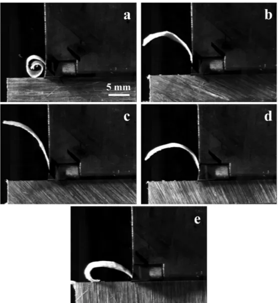
Fig. 6 shows that the removed chip remains continuous regardless of the fiber orientation. However, flax fiber orientation has an obvious effect on the shape of the removed chip, typically the chip curling. The cutting of flax/PLA composites with a fiber orientation of θ ¼ 0�
gener-ates the highest curled chip. Then, the chip curling is reduced when increasing the fiber orientation up to θ ¼ 45�, and it is increased when
increasing the fiber orientation from θ ¼ 45�to θ ¼ 90�.
The fact that the chip remain continuous for all the cutting config-urations reflects the ductile behavior of flax/PLA composites during the machining operation. This behavior is induced by the combination of the well-known ductile properties of thermoplastic polymers and the elasto- visco-plastic behavior of natural flax fibers [23]. The ductile failure mode of this kind of thermoplastic composites avoids the brittle fracture of the chip during its formation [10].
4.2. Experimental and numerical machining behaviors of flax/PLA composites
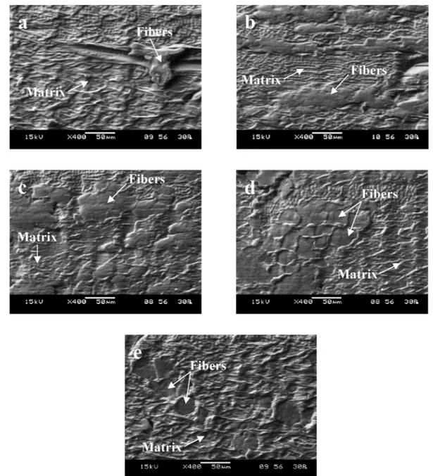
Fig. 7 shows the experimental SEM observations of the machined surfaces of flax/PLA composites at the different considered fiber orien-tations. It can be seen that flax/PLA composites show globally an effi-cient machinability. Indeed, by comparing the microscopic observations of this study and the results of our previous work with flax/poly-propylene (PP) samples [10,13], the fibers shearing of flax/PLA is more efficient with no significant debonding zones. These latter were more important when machining flax/PP and are caused by both the trans-verse deformation of fibers and the failure of the interfaces [10,13]. The main factors that could be behind this behavior are the mechanical and the adhesive properties of the polymer matrices. In fact, when comparing the stress/strain curves of PLA given in Fig. 3(b) and that of PP given in Ref. [13], it is evident that PP matrix exhibits a higher plasticity than that of PLA. Therefore, flax fibers in PP matrix have lower contact stiffness than that of flax fibers in PLA matrix during the cutting operation. The low contact stiffness engenders a high deformation of flax fibers toward the cutting direction which causes an ineffective fiber shearing and, hence, the failure of the interfaces. In the current study, the higher stiffness of PLA matrix, comparing to PP matrix, encounters these issues.
Fig. 6. Fast-cam images of the chip formation during orthogonal cutting of flax/PLA composites at the different considered fiber orientations. (a) θ ¼ 0�, (b) θ ¼ 25�,
It can also be seen that the machined surface with fiber orientation of θ ¼65�(Fig. 7(d)) shows the best fiber shearing since the cross section of
fibers are more obvious than that of the other configurations. This demonstrates that the fiber orientation θ ¼ 65� provides the highest
contact stiffness during the cutting operation which favors the shearing and avoids high plastic deformation. For the fiber orientation θ ¼ 0�,
some detached and torn-off fibers are detected as shown in Fig. 7(a). These phenomena are especially due to the contact location between the cutting edge and the fibers. The fibers oriented toward the cutting di-rection may be sheared, detached or torn-off regarding the location of the cutting edge on the cross-section of each elementary fiber on the fiber bundle.
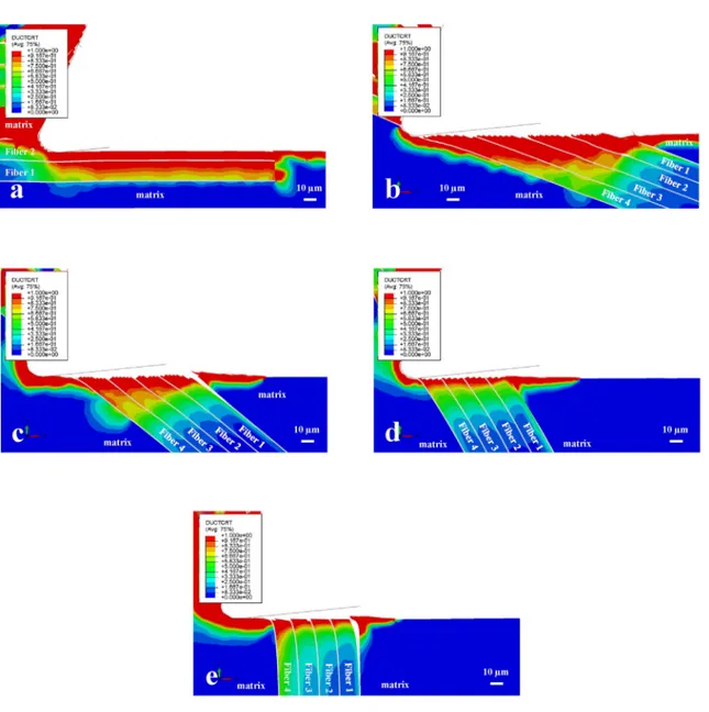
Fig. 8 shows the numerical cutting behavior of the flax/PLA com-posite obtained by the 2D FE micromechanical model. The numerical cutting behavior of flax fibers are similar to that shown in the experi-mental SEM observations. Flax fibers are efficiently sheared without high transverse deformations or high interfaces failure. The micro-mechanical model shows that the orientations θ ¼ 65� generates less
subsurface damages and less interfaces failure. This finding is also
noticed in the SEM observations of Fig. 7(d) where the fibers shape is more obvious than the other configurations. The fact that flax fiber shapes are still obvious in the microscopic observations means that the fibers have not been significantly deformed and damaged during the cutting operation. For θ ¼ 0�, the FE model does not reproduce the
detachment or the torn-off of fibers because the cutting edge has been placed on the middle of the cross section of the fiber 2 in Fig. 8(a). The resulting fiber behavior should be shearing rather than detachment or torn-off.
4.3. Effect of micro-friction coefficient on numerical machining forces 4.3.1. Hypothesis of isotropic micro-friction
Fig. 9 presents the results of numerical cutting and thrust forces at different isotropic micro-friction values in order to compare with the experimental outputs. From the graph of cutting forces in Fig. 9(a), it can be seen that the numerical cutting forces correspond to the experimental results in terms of trend and magnitude. Moreover, the variation of the micro-friction coefficient has not a significant effect on the numerical Fig. 7. Typical SEM images of machined surfaces of flax/PLA composites at the different considered fiber orientations. (a) θ ¼ 0�, (b) θ ¼ 25�, (c) θ ¼ 45�, (d) θ ¼
cutting force results. For the thrust forces presented in Fig. 9(b), the numerical results show a high variation in function of the isotropic micro-friction. At θ ¼ 90�and θ ¼ 65�, the numerical thrust force
de-creases significantly by the increase of the micro-friction from 0.1 to 0.5 to be far from the experimental value. This could explain the difference in magnitude of the thrust forces observed in Ref. [13] since the micro-frictions that were used are μf ¼0.5 and μm ¼0.4. At θ ¼ 45�,
there is no significant effect of the micro-friction on the thrust force. On the other hand, the lowest value of the isotropic micro-friction (μf ¼μm
¼0.1) generates the highest values of the numerical thrust force in the
case of θ ¼ 0�and θ ¼ 25�. Beyond this lowest micro-friction value, the
numerical thrust force increases by increasing the micro-friction at θ ¼ 0� while the effect of the micro-friction is insignificant at θ ¼ 25�.
Consequently, the numerical thrust forces have a good correlation with the experimental results when the value of the isotropic micro-friction is equal to 0.1.
4.3.2. Hypothesis of anisotropic micro-friction
Fig. 10 shows that the numerical cutting forces have a similar behavior as the hypothesis of an isotropic micro-friction presented in Fig. 8. FE model showing the ductile criterion map of the orthogonal cutting of flax/PLA composite at the different considered fiber orientations. (a) θ ¼ 0�, (b) θ ¼
25�, (c) θ ¼ 45�, (d) θ ¼ 65�, and (e) θ ¼ 90�.
Fig. 9(a). The micro-friction between the cutting tool and flax fibers does not affect the numerical cutting forces. However, the value 0.1 of micro- friction between the cutting tool and the PLA matrix leads to decrease slightly the numerical cutting forces at θ ¼ 0�and, then, to get a better fit
with the experimental value as shown in Fig. 10(a).
For the numerical thrust forces, Fig. 11 shows that, at each value of μm, the numerical results present a high variability in function of μf as
the hypothesis of an isotropic micro-friction presented in Fig. 9(b). Moreover, increasing μm leads to an increase of the divergence between
the numerical and the experimental results. Fig. 11(a) reveals that a good agreement between the numerical and the experimental results for thrust forces is reached for an isotropic micro-friction between the cutting tool and the NFRP components where μf ¼μm ¼0.1.
4.4. Effect of fiber orientation on the experimental machined surface topography
To qualify the effect of fiber orientation on the machinability of flax/
PLA composites, optical interferometer has been used to capture the machined surface topography. As explained in section 1, The topo-graphic image size should correspond to the considered fibrous structure size in order to be on the relevant scale for an efficient topographic analysis. The fibrous structure size in the case of the considered flax/PLA composites are continuous unidirectional bundles of flax fibers. The average diameter of the flax fiber bundles in flax/PLA composites is about 150�50 μm. The objective of the interferometer has been adapted
to be as close as possible to this scale range. Therefore, an objective with a magnification of � 20 is used to get topographic images of 153 � 204 μm2. The quantification of these measurements with the arithmetic
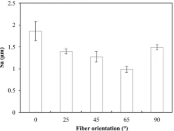
mean of the surface roughness (Sa) is given in Fig. 12.
The cutting behavior of flax fibers within PLA matrix shown in Section 4.2 is accurately quantified by the topographic measurements of
Fig. 12. Indeed, the machined surfaces with θ ¼ 65�generate the lowest
surface roughness thanks to the efficient shearing of flax fibers as clearly shown in the SEM images of Fig. 7. The FE numerical model predicts the same finding where the cutting configuration with θ ¼ 65�produces less
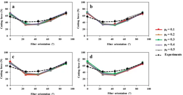
Fig. 10. Comparison between experimental and numerical cutting forces at different values of anisotropic micro-friction. (a) μm ¼ 0.1, (b) μm ¼ 0.2, (c) μm ¼ 0.3, and (d) μm ¼ 0.4.
Fig. 11. Comparison between experimental and numerical thrust forces at different values of anisotropic micro-friction. (a) μm ¼ 0.1, (b) μm ¼ 0.2, (c) μm ¼ 0.3, and
damages in fibers without significant debonding in the interfaces as shown in Fig. 8(d). On the other hand, the random cutting behavior of flax fibers at θ ¼ 0�induces high irregularities on the topographic signals
which induces the highest surface roughness.
5. Conclusions
In this paper, a 2D finite element model for machining of natural fiber composites at microscale has been investigated and optimized in order to reproduce efficiently the machining forces. The optimization approach was based on the investigation of the micro-friction between the cutting tool edge and the two main components of the flax/PLA composite. The following conclusions can be drawn:
�The numerical cutting forces provided by the micromechanical model correspond to the experimental results and are not affected by the variation of the micro-friction between the tool and the com-posite phases.
�The numerical thrust forces provided by the micromechanical model are significantly affected by the micro-friction between the tool and the composite phases.
�The micromechanical model shows that an isotropic micro-friction coefficient of 0.1 between the carbide cutting insert and the com-posite phases allows a good correlation of the thrust forces with the experimental results.
�The micromechanical model can reproduce qualitatively the cutting behavior of natural fibers at different fiber orientations.
�Based on the FE model and the experimental results, the cutting configuration with a fiber orientation of 65�, with respect to the
cutting direction, offers the best surface quality with an efficient shearing of flax fibers and the lowest surface roughness.
Declaration of competing interest
The authors declare that they have no known competing financial interests or personal relationships that could have appeared to influence the work reported in this paper.
CRediT authorship contribution statement
Faissal Chegdani: Conceptualization, Methodology, Writing -
orig-inal draft. Mohamed El Mansori: Conceptualization, Supervision, Writing - review & editing. Amen-Allah Chebbi: Investigation, Validation.
roll bar with particular emphasis on the environment. Int J Precis Eng Manuf Green Technol 2018;5:111–9. https://doi.org/10.1007/s40684-018-0012-y.
[6] Rajmohan T, Vinayagamoorthy R, Mohan K. Review on effect machining parameters on performance of natural fibre–reinforced composites (NFRCs). J Thermoplast Compos Mater 2019;32:1282–302. https://doi.org/10.1177/ 0892705718796541.
[7] Vinayagamoorthy R, Rajmohan T. Machining and its challenges on bio-fibre reinforced plastics: a critical review. J Reinforc Plast Compos 2018;37:1037–50.
https://doi.org/10.1177/0731684418778356.
[8] Lotfi A, Li H, Dao DV, Prusty G. Natural fiber–reinforced composites: a review on material, manufacturing, and machinability. J Thermoplast Compos Mater 2019.
https://doi.org/10.1177/0892705719844546. 089270571984454.
[9] Wang D, Onawumi PY, Ismail SO, Dhakal HN, Popov I, Silberschmidt VV, et al. Machinability of natural-fibre-reinforced polymer composites: conventional vs ultrasonically-assisted machining. Compos Appl Sci Manuf 2019;119:188–95.
https://doi.org/10.1016/J.COMPOSITESA.2019.01.028.
[10] Chegdani F, Mansori M El. Mechanics of material removal when cutting natural fiber reinforced thermoplastic composites. Polym Test 2018;67:275–83. https:// doi.org/10.1016/j.polymertesting.2018.03.016.
[11] Chegdani F, El Mansori M. New multiscale Approach for machining analysis of natural fiber reinforced bio-composites. J Manuf Sci Eng Trans ASME 2019;141: 11004. https://doi.org/10.1115/1.4041326.
[12] Hossain R, Islam A, Vuure A Van, Verpoest I. Processing dependent flexural strength variation of jute fiber reinforced epoxy composites. J Eng Appl Sci 2013;8: 513–8.
[13] Chegdani F, El Mansori M, Bukkapatnam S TS, Reddy JN. Micromechanical modeling of the machining behavior of natural fiber-reinforced polymer composites. Int J Adv Manuf Technol 2019;105:1549–61. https://doi.org/ 10.1007/s00170-019-04271-3.
[14] Arola D, Ramulu M. Orthogonal cutting of fiber-reinforced composites: a finite element analysis. Int J Mech Sci 1997;39:597–613. https://doi.org/10.1016/ S0020-7403(96)00061-6.
[15] Lasri L, Nouari M, El Mansori M. Modelling of chip separation in machining unidirectional FRP composites by stiffness degradation concept. Compos Sci Technol 2009;69:684–92. https://doi.org/10.1016/J.
COMPSCITECH.2009.01.004.
[16] Chegdani F, Wang Z, El Mansori M, Bukkapatnam STS. Multiscale tribo-mechanical analysis of natural fiber composites for manufacturing applications. Tribol Int 2018;122:143–50. https://doi.org/10.1016/j.triboint.2018.02.030.
[17] Chegdani F, El Mansori M, Bukkapatnam STS, El Amri I. Thermal effect on the tribo-mechanical behavior of natural fiber composites at micro-scale. Tribol Int 2019. https://doi.org/10.1016/j.triboint.2019.06.024.
[18] Abaqus analysis user’s manual. Abaqus 6.11 doc. Providence, RI, USA: Dassault Syst�emes Simulia Corp.; 2011.
[19] Nayak D, Singh I, Bhatnagar N, Mahajan P. An analysis of machining induced damages in FRP composites — a micromechanics finite element approach. AIP Conf. Proc. 2004;712:327–31. https://doi.org/10.1063/1.1766545. AIP. [20] Santiuste C, Soldani X, Migu�elez MH. Machining FEM model of long fiber
composites for aeronautical components. Compos Struct 2010;92:691–8. https:// doi.org/10.1016/J.COMPSTRUCT.2009.09.021.
[21] Ghidossi P, El Mansori M, Pierron F. Edge machining effects on the failure of polymer matrix composite coupons. Compos Appl Sci Manuf 2004;35:989–99.
https://doi.org/10.1016/j.compositesa.2004.01.015.
[22] Baley C. Analysis of the flax fibres tensile behaviour and analysis of the tensile stiffness increase. Compos Appl Sci Manuf 2002;33:939–48. https://doi.org/ 10.1016/S1359-835X(02)00040-4.
[23] Charlet K, Baley C, Morvan C, Jernot JP, Gomina M, Br�eard J. Characteristics of Herm�es flax fibres as a function of their location in the stem and properties of the derived unidirectional composites. Compos Appl Sci Manuf 2007;38:1912–21.
https://doi.org/10.1016/j.compositesa.2007.03.006.
[24] Hearle JWS. The fine structure of fibers and crystalline polymers. III. Interpretation of the mechanical properties of fibers. J Appl Polym Sci 1963;7:1207–23. https:// doi.org/10.1002/app.1963.070070403.
[25] Shah DU, Schubel PJ, Licence P, Clifford MJ. Determining the minimum, critical and maximum fibre content for twisted yarn reinforced plant fibre composites. Compos Sci Technol 2012;72. https://doi.org/10.1016/J.
COMPSCITECH.2012.08.005. 1909–17.
[26] Yang J, Pan H, Li X, Sun S, Zhang H, Dong L. A study on the mechanical, thermal properties and crystallization behavior of poly(lactic acid)/thermoplastic poly (propylene carbonate) polyurethane blends. RSC Adv 2017;7:46183–94. https:// doi.org/10.1039/C7RA07424G.
Fig. 12. Arithmetic surface roughness of machined surfaces of flax/PLA
[27] Dittenber DB, GangaRao HVS. Critical review of recent publications on use of natural composites in infrastructure. Compos Appl Sci Manuf 2012;43:1419–29.
https://doi.org/10.1016/j.compositesa.2011.11.019.
[28] Cardoso RPR, Adetoro OB. A generalisation of the Hill’s quadratic yield function for planar plastic anisotropy to consider loading direction. Int J Mech Sci 2017; 128–129:253–68. https://doi.org/10.1016/j.ijmecsci.2017.04.024.
[29] Panamoottil SM, Das R, Jayaraman K. Towards a multiscale model for flax composites from behaviour of fibre and fibre/polymer interface. J Compos Mater 2017;51:859–73. https://doi.org/10.1177/0021998316654303.
[30] Hooputra H, Gese H, Dell H, Werner H. A comprehensive failure model for crashworthiness simulation of aluminium extrusions. Int J Crashworthiness 2004; 9:449–64. https://doi.org/10.1533/ijcr.2004.0289.
[31] Danas K, Ponte Casta~neda P. Influence of the Lode parameter and the stress triaxiality on the failure of elasto-plastic porous materials. Int J Solid Struct 2012; 49:1325–42. https://doi.org/10.1016/J.IJSOLSTR.2012.02.006.
[32] Venu Gopala Rao G, Mahajan P, Bhatnagar N. Machining of UD-GFRP composites chip formation mechanism. Compos Sci Technol 2007;67:2271–81. https://doi. org/10.1016/J.COMPSCITECH.2007.01.025.
[33] Lee J-S, Jang J, Lee B-W, Choi Y, Lee SG, Kwon D. An instrumented indentation technique for estimating fracture toughness of ductile materials: a critical indentation energy model based on continuum damage mechanics. Acta Mater 2006;54:1101–9. https://doi.org/10.1016/J.ACTAMAT.2005.10.033. [34] Park K, Choi H, Paulino GH. Assessment of cohesive traction-separation
relationships in ABAQUS: a comparative study. Mech Res Commun 2016;78:71–8.
https://doi.org/10.1016/J.MECHRESCOM.2016.09.004.
[35] Camanho PP, Davila CG, de Moura MF. Numerical simulation of mixed-mode progressive delamination in composite materials. J Compos Mater 2003;37: 1415–38. https://doi.org/10.1177/0021998303034505.
[36] Le Duigou A, Baley C, Grohens Y, Davies P, Cognard J-Y, Cr�each’cadec R, et al. A multi-scale study of the interface between natural fibres and a biopolymer. Compos Appl Sci Manuf 2014;65:161–8. https://doi.org/10.1016/J. COMPOSITESA.2014.06.010.
[37] Le Duigou A, Davies P, Baley C. Interfacial bonding of Flax fibre/Poly(l-lactide) bio-composites. Compos Sci Technol 2010;70:231–9. https://doi.org/10.1016/J. COMPSCITECH.2009.10.009.
[38] Merchant ME. Mechanics of the metal cutting process. I. Orthogonal cutting and a type 2 chip. J Appl Phys 1945;16:267. https://doi.org/10.1063/1.1707586. [39] Wang F, Yin J, Ma J, Jia Z, Yang F, Niu B. Effects of cutting edge radius and fiber
cutting angle on the cutting-induced surface damage in machining of unidirectional CFRP composite laminates. Int J Adv Manuf Technol 2017;91: 3107–20. https://doi.org/10.1007/s00170-017-0023-9.
[40] Sauer K, Witt M, Putz M. Influence of cutting edge radius on process forces in orthogonal machining of carbon fibre reinforced plastics (CFRP). Procedia CIRP 2019;85:218–23. https://doi.org/10.1016/J.PROCIR.2019.09.042.
[41] Ulutan D, €Ozel T. Methodology to determine friction in orthogonal cutting with application to machining titanium and nickel based alloys. In: ASME 2012 Int. Manuf. Sci. Eng. Conf., American Society of Mechanical Engineers; 2012. p. 327–34. https://doi.org/10.1115/MSEC2012-7275.
[42] Albrecht P. New developments in the theory of the metal-cutting process: Part I. The ploughing process in metal cutting. J Eng Ind 1960;82:348. https://doi.org/ 10.1115/1.3664242.
[43] Rao GVG, Mahajan P, Bhatnagar N. Micro-mechanical modeling of machining of FRP composites – cutting force analysis. Compos Sci Technol 2007;67:579–93.