1
Development of a method for determining the relevant
geomechanical parameters for evaluating the hydraulic erodibility
of rock
Lamine Boumaizaa*, Ali Saeidia, and Marco Quirionb
aDépartement des Sciences appliquées, Université du Québec à Chicoutimi, Chicoutimi
(Québec), G7H 2B1, Canada
bExpertise en barrages, Direction Barrages et infrastructures, Hydro-Québec, Montréal,
(Québec), H2Z 1A4, Canada
*Corresponding author: E-mail address: lamine.boumaiza@uqac.ca (L. Boumaiza)
Abstract
Among the methods used for evaluating the potential hydraulic erodibility of rock, the most common are those based on the correlation between the force of flowing water and the capacity of a rock to resist erosion, such as Annandale’s and Pells’s methods. The capacity of a rock to resist erosion is evaluated based on erodibility indices that are determined from specific geomechanical parameters of a rock mass. These indices include the unconfined compressive strength of rock, rock block size, joint shear strength, a block’s shape and orientation relative to the direction of flow, joint openings, and the nature of the surface to be potentially eroded. However, it is difficult to determine the relevant geomechanical parameters for evaluating the hydraulic erodibility of rock. The assessment of eroded unlined spillways of dams has shown that the capacity of a rock to resist erosion is not accurately evaluated. Using more than 100 case studies, we develop a method to determine the relevant geomechanical parameters for evaluating the hydraulic erodibility of rock in unlined spillways. The unconfined compressive strength of rock is found not to be relevant parameter for evaluating the hydraulic erodibility of rock. On the other hand, we find that the use of three-dimensional block volume measurements, instead of the block size factor used in Annandale’s method, improves the rock block size estimation. Furthermore, the parameter representing the effect of a rock block’s shape and orientation relative to the direction of flow, as considered in Pells’s method, is more accurate than the parameter adopted by Annandale’s method.
Keywords: Rock mass, Hydraulic erodibility, Geomechanical parameters, Rock block size, Annandale’s method, Pells’s method, Kirsten’s index, Erosion level
2 Symbol notation list
a1: Longest dimension of a rock block (m)
a3: Shortest dimension of a rock block (m)
Di: Erosion level
Edoa: Erosion, discontinuity orientation adjustment
eGSI: Erodibility geological strength index GSI: Geological strength index
i: Erosion level class
Ja: Joint surface alteration number
Jn: Joint set number
Jo: Joint opening (mm)
Jr: Joint roughness number
Js: Relative block structure
Jv: Number of joints intersecting a volume of 1 m³ Kb: Rock block size number
Kd: Joint shear strength number
LF: Likelihood factor
Ms: Compressive strength number
N: Kirsten’s index
ni: Number of study cases of a given erosion level
NPES: Nature of the potentially eroding surface nt: Total number of study cases
Pa: Available hydraulic stream power (kW/m2)
Pi: Probability of erosion
RF: Relative importance factor RMR: Rock mass rating system RMEI: Rock mass erosion index RMi: Rock mass index
RMSE: Root mean square error (%) RQD: Rock quality designation Sa: Average joint spacing (m) S1: Spacing in joint set (m)
UCS: Unconfined compressive strength (MPa)
μD: Mean erosion level for a given hydraulic steam power category
Vb: Rock block volume (m3)
1: Angles between joint sets (°)
β: Block shape factor λn: Joint frequency
3 1 Introduction
Many rock mass classification systems used in engineering were developed during the last century. The most common are the rock mass rating (RMR) system (Bieniawski, 1973), the Q-system, also known as the Norwegian Geotechnical Institute classification (Barton et al., 1974), the geological strength index (GSI) proposed by Hoek et al. (1995), and the rock mass index (RMi) system (Palmstrom, 1996). These classification systems were developed for multiple purposes, including underground excavation stability and support design. Furthermore, some have been used to develop related indices to evaluate the excavatability of earth materials, such as Weaver’s classification (Weaver, 1975), which was based on the RMR system, and Kirsten’s index (Kirsten, 1982), which includes several of parameters used in the Q-system.
During the Cincinnati Symposium (Kirkaldie, 1988) that focused on engineering rock mass classification systems, it was proposed that the mechanical excavatability and the hydraulic erodibility of earth materials could be considered as similar processes (Moore and Kirsten 1988). Van Svhalkwyk (1989), Pitsiou (1990), and Moore (1991) then demonstrated that the existing rock mass classification systems used for evaluating the mechanical excavatability of rock incorporate most of parameters that affect the hydraulic erodibility of rock. The term “ erodibility ” is used here to describe significant localized erosion of rock that occurs when the rock is submitted to hydraulic erosive power. Van Schalkwyk et al. (1994) tested several rock mass characterization indices for evaluating the hydraulic erodibility of rock, and they found that the indices generated similar results. However, Kirsten's index is more accurate (Pells, 2016a). This index, initially developed to evaluate the excavatability of earth materials, has since been adopted for assessing the hydraulic erodibility of earth materials where the “direction of excavation” of the original index has been replaced by the “direction of flow”
4 (Annandale, 2006, 1995; Annandale and Kirsten, 1994; Doog, 1993; Kirsten et al., 2000; Pitsiou, 1990; Van Schalkwyk et al., 1994). In these cited works, the assessment of hydraulic erodibility is based on a correlation between the erosive force of flowing water and the capacity of the rock to resist the erosive force1. The erosive force of flowing water is the hydraulic
energy, expressed in kW/m2, generated by the flowing water. This erosive force is usually
called the available hydraulic stream power (Pa). For its part, the resistance capacity of rock
can be evaluated using the Kirsten’s index (Kirsten, 1988, 1982), which is determined according to certain geomechanical factors related to the intact rock and the rock mass, such as the unconfined compressive strength (UCS) of rock (Ms), the rock block size (Kb), the joint
shear strength (Kd), and the relative block structure (Js), which considers the effect of a block’s
shape and orientation relative to the direction of excavation. Kirsten’s index (N) can be calculated according to Eq. (1):
N = Ms · Kb ·Kd ·Js (1)
Although there are several developed methods using this correlation approach, Annandale’s method (Annandale, 2006, 1995) is the most common (Castillo and Carrillo, 2016; Hahn and Drain, 2010; Laugier et al., 2015; Mörén and Sjöberg, 2007; Pells et al., 2015; Rock, 2015), and this method has been validated in a series of laboratory tests (Annandale et al., 1998; Kuroiwa et al., 1998; Wittler et al., 1998). Recently, Pells (2016a) proposed two other indices to assess the capacity of rock to resist flowing water. The first, eGSI, represents a modification of GSI previously proposed by Hoek et al. (1995) to characterize the rock mass environment. When the GSI index is determined using the RMR system, the discontinuity orientation factor is removed from RMR (Bieniawski, 1976). Pells (2016a) proposed the eGSI index to include a
1 As noted in Pells (2016a), methods to characterize the “erosive capacity” of a flow and relate it to the “erosive resistance” of the earth or rock
5 new discontinuity orientation adjustment factor (Edoa) to represent the effect of a rock block’s
shape and orientation relative to the direction of flow (Eq. 2).
eGSI = GSI + Edoa (2)
The second index proposed by Pells (2016a) is the RMEI (rock mass erosion index). It can be determined based on the relative importance factor (RF) and likelihood factor (LF) as presented in Eq. (3). The prefixes P1 to P5 in Eq. (3) are various sets of parameters that represent, respectively, the kinematically viable mechanism for detachment, the nature of the potentially eroding surface, the nature of the defects, the spacing of the basal defect, and the block shape (Pells 2016a).
RMEI =(RFP1.LFP1).(RFP2.LFP2).[(RFP3.LFP3)+(RFP4.LFP4)+(RFP5.LFP5)] (3)
Bieniawski (1973) showed that rock mass strength is controlled mostly by joint intensity and joint spacing. Even though the rock substance itself may be strong, impermeable, or both, systems of joints create significant weaknesses and favor fluid conductivity (Goodman 1993). Boumaiza et al. (2017) argued that the UCS of rock could beget a less important impact on the shifting-up of erodibility class. Pells (2016a) considered that the UCS of rock plays a very limited role in the erodibility of fractured rock masses. For example, spectacular erosion events occurred in rock having high UCS values at Copeton Dam in Australia, where a 20 m deep erosion gully was formed, and at the Mokolo Dam in South Africa, where a 30 m deep erosion gully was produced (Pells, 2016a). However, compared to other considered parameters, Kirsten’s index is determined to a great extent by the UCS rating having values ranging from 0.87 to 280 MPa.
Pells et al. (2017a) argued that at the time of its development, the RQD (rock quality designation) parameter, used as a part of the Kb factor, was developed for a specific application
6 and that this parameter is sometimes applied inconsistently in practice. Accordingly, Pells (2016a) recommends use of the Marinos & Hoek (2000) chart to determine GSI (also used to determine the eGSI index), as it does not consider the UCS of the rock nor the RQD. However, this chart remains semi-qualitative, and any subsequent evaluation can be greatly influenced by the judgment of the analyst. Furthermore, it was not developed to assess the hydraulic erodibility of rock. It does not incorporate details on joint openings (Jo) that can play a
determining role in the hydraulic erodibility process. Pells (2016a) included Jo and other
geological parameters, such as the nature of the potentially eroding surface (NPES), within the RMEI classification. NPES is deemed as an important parameter in RMEI classification, more so than other considered parameters, such as joint spacing and block shape (Pells 2016a). Nonetheless, these existing rock mass indices fail to represent the mechanisms of erosion observed in field investigations.
The Js parameter included in Kirsten’s index is mathematically quantified based on the effect of
a block’s shape and orientation relative to the direction of excavation. This parameter was, furthermore, adopted by other systems developed to evaluate the excavatability of earth materials (Scoble et al. 1987, Hadjigeorgiou and Poulin 1998). Pells (2016a) argued, based on the field observations of multiple eroded spillways and laboratory experiments, that the Js
values proposed by Kirsten (1982) for assessing mechanical excavatability of earth materials are not intuitively representative of an assessment of hydraulic erodibility. Furthermore, as set by Kirsten, its rating from 0.37–1.5 has only a subtle impact on the value of Kirsten’s index compared to the UCS rating of rock that ranges from 0.87–280. For this purpose, Pells (2016a) proposed the Edoa factor to represent the effect of the block’s shape and orientation relative to
Q-7 system (Barton et al., 1974), argued that the block size factor Kb, which is included in Kirsten’s
index, provides no meaningful quantification of rock block size. Accordingly, Palmstrom (2005) and Palmstrom and Broch (2006) stated that using block volume (Vb) instead of the Kb
parameter would improve the quality of Q-system results. Grenon and Hadjigeorgiou (2003) have also concluded, from in-situ investigations in Canadian mines, that Kb is an inaccurate
parameter for characterizing block size.
In summary, the key geomechanical parameters to be used for assessing the hydraulic erodibility of rock remain uncertain. The UCS of rock, favored by Kirsten (1982) as a relevant parameter of rock mass competence, is deemed as being less relevant by Pells (2016a) and others. The Kb parameter used in Kirsten’s index as an indication of block size is also deemed
as inappropriate by some, including Grenon and Hadjigeorgiou (2003). Although Jo could have
an important role in the assessment of the hydraulic erodibility of rock, this parameter was not considered directly by Kirsten’s index, and it was ignored completely by the eGSI index when GSI is determined using Marinos & Hoek's (2000) chart. As well, values for the Js parameter,
as proposed by Kirsten (1982) for assessing the mechanical excavatability of earth materials, are seen by Pells (2016a) as having no intuitively representative values for assessing hydraulic erodibility. Furthermore, NPES is deemed to be a relevant parameter for evaluating the hydraulic erodibility of rock. In short, there exists no clear consensus on what geomechanical parameters are indeed relevant for evaluating the hydraulic erodibility of rock.
This paper presents a method for determining the relevant geomechanical parameters when evaluating the hydraulic erodibility of rock. This method is described in the second section where several geomechanical parameters, such as UCS, Kb, Kd, Js, Jo, NPES, Vb, and Edoa, are
8 case studies and coupled with our novel approach demonstrate those geomechanical parameters that are relevant for evaluating the hydraulic erodibility of rock (Section 3). Section 4 presents a validation process of the selected parameters.
2 Description of the developed method
The proposed method for determining the relevant geomechanical parameters for evaluating the hydraulic erodibility of rock is summarized in Fig. 1. Each methodological step is described in the following subsections.
2.1 Step 1 - Establishing a dataset and an erosion-level scale
Step 1, establishing a dataset (Fig. 1), consists of collecting the data from case studies conducted on rocky dam spillways. This data includes all available information related to the geomechanical parameters that characterize rock mass, the Pa, and the observed condition of
erosion. Table 1 summarizes the geomechanical parameters used by Pells (2016a) to develop the two erodibility indices of eGSI and RMEI. Some of the geomechanical parameters considered in Pells’s erodibility indices are also included in Kirsten’s index. Consequently, we also selected geomechanical parameters considered in Kirsten’s index (Kirsten, 1982) for our dataset. For their parts, Jo and NPES are also included in the dataset, although they are not
directly included in Kirsten’s index. As Kb is an inaccurate parameter for characterizing block
size (Palmstrom, 2005), we retained Vb as a parameter to be analyzed. Finally, Edoa is deemed
synonymous to Js for determining the effect of a rock block’s shape and orientation relative to
the direction of flow (Pells, 2016b; Pells et al., 2017b); we therefore included this parameter to verify its effectiveness compared to that of Js. In summary, we retained the geomechanical
parameters of Ms, Kb, Kd, Js, Jo, NPES, Vb, and Edoa. These parameters will be analyzed for
9 Fig. 1. Algorithm for determining the relevant geomechanical parameters for evaluating the
hydraulic erodibility of rock.
Establishment of a dataset and erosion level scale Selection of a geomechanical parameter
Determination of the mean level of erosion for a given Pa
Selection of relevant geomechanical parameters according to the sensitivity curves to erodibility YES NO Selection of another geomechanical parameter
Classification of the selected geomechanical parameter
Analysis of sensitivity curves to erodibility YES All geomechanical parameter classes are evaluated All geomechanical parameters are analyzed NO 1 2 3 4 5 6 7 8
10 Table 1. Summary of the considered geomechanical parameters.
Index Conditions Parameters
eGSI 1
Strength of rock UCS
Joints condition RQD Joint spacing Joint opening Roughness Infilling gouge Weathering Rock block condition2 Dipping Shape
Orientation
RMEI
Joint condition
Number of joint sets Dipping Orientation Roughness UCS of joints Joint opening Joint spacing
Rock block condition Shape
Nature of the potentially eroding surface
Protrusion of joints Opening of defects
Weathering
N
Strength of rock UCS
Joint condition
RQD
Number of joint sets Roughness Infilling gouge Rock block condition
Shape Dipping Orientation 1: eGSI parameters are specified according to the RMR system.
2: Considered as part of the Edoa parameter.
The field data collected from more than 100 case studies conducted by Pells (2016a) are presented in Appendix 1. These case studies, conducted on unlined rocky spillways of selected dams in Australia and South Africa, were selected as they provide complete data for the retained geomechanical parameters (Ms, Kb, Kd, Js, Jo, NPES, Vb, and Edoa), the Pa, and the
11 The erosion-level scale used in this study, as part of Step 1 (Fig. 1), is based on the description of the erosion condition as defined by Pells (2016a). Erosion condition is determined using the maximum depth and extension of the eroded gully (Table 2).
Table 2. Erosion condition description (Pells, 2016a). Max. depth
(m)
General extent
(m3/100 m2) Descriptor Erosion level
<0.3 <10 Negligible 1
0.3–1 1–30 Minor 2
1–2 30–100 Moderate 3
2–7 100–350 Large 4
>7 >350 Extensive 5
2.2 Step 2 - Selection of a geomechanical parameter
The retained geomechanical parameters (Ms, Kb, Kd, Js, Jo, NPES, Vb, and Edoa) are assessed
individually. Therefore, Step 2 (Fig. 1) consists of selecting one geomechanical parameter from the set of retained parameters. This selected parameter is then analyzed in Steps 3–7 (Fig. 1). This process is repeated for each of the retained parameters.
2.3 Step 3 - Classification of the selected geomechanical parameter
Once a geomechanical parameter is considered for analysis (Step 2, Fig. 1), this parameter is then classified in Step 3. The objective of Step 3 is to verify the level of erosion (1 to 5; Table 2) when a given rock mass is submitted to various Pa. The classification of the geomechanical
parameters relies on existing classifications from the literature or our proposed statistical classifications. In the following subsections, we describe the classifications of all retained geomechanical parameters (Ms, Kb, Kd, Js, Jo, NPES, Vb, and Edoa).
12 2.3.1 Classification of the UCS of rock
Ms included in Kirsten’s index is determined according to the UCS of rock, which can be
estimated by performing an unconfined compressive stress test on an intact rock sample (Annandale, 2006). We use two common UCS scales (Tables 3 and 4).
Table 3. UCS classification of Jennings et al. (1973).
Class UCS (MPa) Description
1 1.7–3.3 Very soft rock
2 3.3–13.2 Soft rock
3 13.2–26.4 Hard rock
4 26.4 –106 Very hard rock
5 >106 Extremely hard rock
Table 4. UCS classification adopted from Bieniawski (1989, 1973).
Class UCS (MPa) Description
1 1–5 Very low strength
2 5–25 Low strength
3 25 –50 Medium strength
4 50–100 High strength
5 100–250 Very high strength
6 >250 Extremely high strength
2.3.2 Classification of rock block size Classification of Kb
Block size is an extremely important parameter for evaluating rock mass behavior (Barton, 1990; ISRM, 1978). The most common indicator of block size was introduced by Cecil (1970)
who combined the RQD index with the joint set number (Jn) to create the quotient Kb (RQD/Jn).
This quotient was later adopted by Barton et al. (1974) into the Q-system and by Kirsten (1982)
for his excavatability index. However, RQD measurements have several limitations (Grenon and Hadjigeorgiou, 2003; Palmstrom et al., 2002; Pells et al., 2017a). This parameter is included in our analyzed geomechanical parameters to verify if it can be retained as a relevant parameter for evaluating the hydraulic erodibility of rock (as previously maintained). As RQD
13 can vary from 5%–100% and Jn values vary from 1–5 (Kirsten, 1988, 1982), consequently the
Kb values range from 1–100. However, there is no existing classification system for Kb. The Kb
classification framework proposed in this study is based on the statistical distribution of Kb that
was established through evaluating the case studies. The most representative normal distribution of Kb data is obtained based on the interval values presented in Fig. 2. Accordingly,
five classes of Kb are defined (Table 5).
Fig. 2. The statistical distribution of Kb values from the case studies of Pells (2016a).
Table 5. Proposed Kb classification.
Class Kb 1 0–7 2 7–14 3 14–21 4 21–28 5 >28 0 5 10 15 20 25 30 0-7 7-14 14-21 21-28 >28 C as e st u d ie s (% ) Kbinterval values
14 Classification of Vb
Palmstrom (2005) stated that using three-dimensional block volume measurements improves the characterization of block size. The block volume classification of Palmstrom (1996, 1995), presented in Table 6, is adopted for this study. Furthermore, we apply three methods (Methods 1, 2, and 3) to characterize rock block volume (Palmstrom, 2005).
Table 6. Classification of rock block volume (Palmstrom, 1995).
Vb (m3) Description 0.0002–0.01 Small 0.01–0.2 Moderate 0.2–10 Large >10 Very large Method 1
When the average joint spacing is used rather than the abundance of joint sets, the following expression is used to determine Vb (m3):
Vb = Sa3 (4)
where Sa is the average joint spacing equal to (S1+S2+S3+Sn)/n, where S1, S2, S3…Sn is the
average spacing for each of the joint sets. Method 2
When three joint sets occur, the following expression may be used to determine Vb (m3):
Vb = S1· S2·S3
15 where S1, S2, S3 represent the spacing of the three joint sets, and γ1, γ2, γ3 represent the angles
between the joint sets. Method 3
The block volume may be determined according to:
Vb = β · Jv-3 (6)
where β is the block shape factor obtained through the following equation:
β = 20 + (7a3/a1) (7)
where a3 and a1 are the shortest and longest dimensions of a block, respectively. Jv is defined as
the number of joints intersecting a volume of 1 m³, as determined using Jv = λ1+ λ2+λ3+λn
(where λ1 is the joint frequency of joint set 1).
2.3.3 Classification of joint shear strength
In his index, Kirsten (1982) included Kd, as proposed by Barton et al. (1974); this quotient
represents joint shear strength and is expressed as the ratio Jr/Ja, where Jr is the rating number
corresponding to joint roughness, while Ja is the rating number corresponding to joint surface
alteration. The Jr rating for joint conditions ranges from 0.5–4, whereas the Ja rating varies
from 0.75–18 (Kirsten, 1982). Accordingly, Kd varies from 0.03–5.33; however, there is no
existing classification of Kd. Based on the statistical distribution of Kd (Fig. 3), we determined
16 Fig. 3. The statistical distribution of Kd values from the case studies of Pells (2016a).
Table 7. Proposed Kd classification.
Class Kd
1 0–0.5
2 0.5–1
3 1–1.5
4 1.5–3
2.3.4 Classification of a block’s shape and orientation parameters Classification of Js
The Js parameter included in Kirsten’s index was mathematically quantified according to the
effect of a block’s shape and orientation relative to the direction of excavation. Its rating, as proposed by Kirsten, ranges from 0.37–1.5. As there is no existing classification of Js, we
performed a statistical distribution of the case studies data (Fig. 4). We determined five classes for Js(Table 8). Class 4 (Table 8) is defined by the value of 1 given that there are multiple case
studies having a Js value of 1.
0 5 10 15 20 25 30 35 40 0 - 0.5 0.5 - 1 1 - 1.5 1.5 - 3 C as e st u d ie s (% ) Kdinterval values
17 Fig. 4. The statistical distribution of Jsvalues obtained from the case studies of Pells (2016a).
Table 8. Proposed Jsclassification.
Class Js Description
1 0.4–0.6 Highly vulnerable to erosion 2 0.6–0.8 Very vulnerable to erosion 3 0.8–<1 Moderately vulnerable to erosion
4 1 Less vulnerable to erosion
5 >1 Minimally vulnerable to erosion
Classification of Edoa
Pells (2016a) proposed the eGSI index to include a new discontinuity orientation adjustment factor (Edoa) to represent the effect of a rock block’s shape and orientation relative to the
direction of flow (Eq. 2). The process of deriving values for Edoa was inspired from Kirsten’s Js
parameter. However, values were derived purely by a thought experiment. A rock’s vulnerability to significant and ongoing erosion was assessed by taking into consideration the kinematics of block removal and the nature and direction of hydraulic loading, as derived from
0 10 20 30 40 50 60 0.4 - 0.6 0.6 - 0.8 0.8 - <1.0 1.0 >1.0 C as e st u d ie s (% ) Jsinterval values
18 observation at sites and the analysis of numerous tested models (Pells, 2016a). As values of Edoa present the discontinuity orientation factor, they are presented as negative values, such as
those included in the RMR system (Bieniawski, 1976).
The Edoa parameter is included in our list of analyzed geomechanical parameters to verify
whether Edoa can be retained as a relevant parameter and to compare the results with those for
Js. This comparison will confirm which parameter is most representative of the effect of the
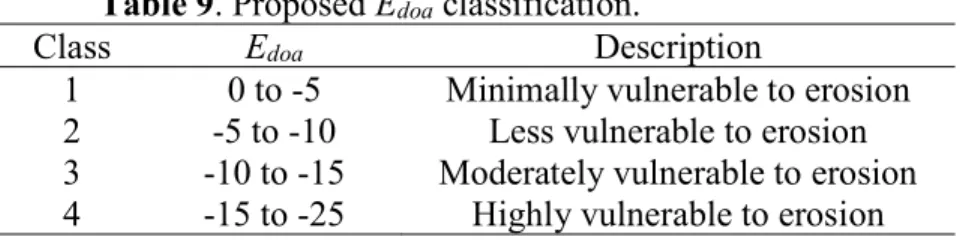
block’s shape and orientation. According to Pells (2016a), Edoa values vary from 0 to -30.
Given that there is no existing classification of Edoa, we assessed a statistical distribution of data
from the case studies (Fig. 5), and we determined four classes for the Edoaparameter (Table 9).
Lower values of Edoa, such as those included in Class 4, indicate that a rock is more vulnerable
to erosion and, consequently, could be susceptible to forms of aggressive erosion.
Fig. 5. The statistical distribution of Edoavalues obtained from the case studies of Pells (2016a).
0 5 10 15 20 25 30 35 0 to -5 -5 to -10 -10 to -15 -15 to -25 C as e st u d ie s (% )
19 Table 9. Proposed Edoaclassification.
Class Edoa Description
1 0 to -5 Minimally vulnerable to erosion 2 -5 to -10 Less vulnerable to erosion 3 -10 to -15 Moderately vulnerable to erosion 4 -15 to -25 Highly vulnerable to erosion
2.3.5 Classification of joint openings
Here, we adopt the joint opening classification of Bieniawski (1989), as presented in Table 10. As some case studiescontain more than three joint sets, characterized by different joint opening dimensions, we use the joint opening of the joint set most sensitive to hydraulic erodibility (the joint set most oriented with the flow direction). As presented in the Appendix 1, some joint set dimensions are characterized by an interval, such as 0.1–0.5 mm. For such cases, the maximum value of the interval is retained for classification purposes.
Table 10. Joint opening classification (Bieniawski, 1989) with our proposed class. Opening (mm) Description Proposed class
<0.1 Very tight 1
0.1–0.25 Tight 2
0.25–0.5 Partly open 3
0.5–2.5 Open 4
2.5–10 Widely open 5
10–100 Very widely open 6
100–1000 Extremely widely open 7
>1000 Cavernous 8
2.3.6 Classification of NPES
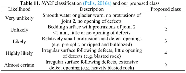
Our classification of NPES (Table 11) is adopted from the RMEI classification (Pells, 2016a). Spillways characterized by a Class 5 in Table 11 are the most sensitive to erosion.
20 Table 11. NPES classification (Pells, 2016a) and our proposed class.
Likelihood Description Proposed class
Very unlikely Smooth water or glacier worn, no protrusions of joint 2, no opening of defects 1 Unlikely Bedding surface with protrusions of joint 2
<1 mm, little or no opening of defects 2 Likely Relatively small protrusions and defect openings (e.g. pre-split, or ripped and bulldozed) 3 Highly likely Irregular surface following defects, little opening of defects (e.g. blasted rock) 4 Almost certain Irregular surface following defects, extensive defect opening (e.g. heavily blasted rock) 5
2.4 Step 4 - Determining mean levels of erosion for given Pa categories
In Step 4, the objective is to verify erosion levels when the same rock mass class (rock mass classes are defined in Tables 3–11) is subjected to various Pa. As there are several case studies
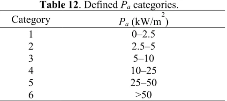
within the same geomechanical class, we determine in Step 4 the mean level of erosion for a given Pa category (Fig. 1). However, there is no existing classification of Pa. Accordingly, we
performed a statistical distribution of data from the case studies (Fig. 6), and we define six Pa
categories (Table 12).
Fig. 6. Statistical distribution of Pa values from the case studies of Pells (2016a).
0 5 10 15 20 25 30 0 - 2.5 2.5 - 5 5 - 10 10 - 25 25 - 50 >50 C as e st u d ie s (% ) PaInterval values
21 Table 12. Defined Pacategories.
Category Pa(kW/m2) 1 0–2.5 2 2.5–5 3 5–10 4 10–25 5 25–50 6 >50
The mean level of erosion for a given Pa category is calculated using Eq. (8) (Saeidi et al.,
2012, 2009), where, in this study, μD represents the mean erosion level for a given hydraulic
steam power category, and Pi is the probability of erosion level Di, where i is ranking of the
erosion level classes from 1 to 5 (Table 2). Pi is calculated according to Eq. 9, where ni is
number of case studies of erosion level Di, and nt is the total number of case studies, both
considered for each Pacategory. An example of how the mean erosion level was calculated is
presented in Table 13. μD = Pi· Di 5 i=1 (8) Pi = ni nt (9)
Table 13. Example of calculating μD
Erosion class Di ni Negligible 1 3 Minor 2 3 Moderate 3 1 Large 4 1 Extensive 5 0 nt 8 μD 2
22 2.5 Step 5 – Evaluating all geomechanical parameter classes
After calculating the mean level of erosion for a Pa category (e.g. for Category 1 of Table 12;
Pa = 0–2.5 kW/m2), the identical process for calculations is then run for all Pa categories listed
in Table 12. Each series of calculations for the Pa categories is run for only a single
geomechanical parameter class (e.g. Class 1 of the NPES classification in Table 11) at a time. Accordingly, a best-fit curve representing the calculated mean level of erosion versus the average of all considered Pa categories are then plotted for this single class of geomechanical
parameter. Step 5 (Fig. 1) aims to runs the identical process of calculations for each class of a single geomechanical parameter (e.g. the calculating process for classes 1 to 5 of NPES classification as indicated in Table 11).
2.6 Step 6 - Analysis of sensitivity curves to erodibility
A best-fit curve here is the line representing the considered points of the calculated mean level of erosion versus the average of all considered Pa categories. For each class of a single
geomechanical parameter, a best-fit curve is traced. These best-curves are considered as the sensitivity curves to erodibility that could produce a synthetic value for the potential level of erosion at a given value of Pa for a specific geomechanical parameter class. These best-fit
curves are used in our subsequent analyses. The main objective of Step 6 (Fig. 1) is to analyze the obtained sensitivity curves. For a geomechanical parameter, the obtained sensitivity curves to erodibility showing a logical sequence can be considered as curves associated with a relevant geomechanical parameter for evaluating the hydraulic erodibility of rock. Otherwise, it can be concluded that the analyzed geomechanical parameter cannot be considered as a relevant parameter.
23 2.7 Steps 7 and 8 – Analyse of all geomechanical parameters and the selection of the
relevant geomechanical parameters
Step 7 consists of analyzing all retained geomechanical parameters (Ms, Kb, Kd, Js, Jo, NPES,
Vb, and Edoa) via the process described in the previous steps. Each retained parameter will have
a specific sensitivity curves to erodibility. Step 8 selects the relevant geomechanical parameters for evaluating the hydraulic erodibility of rock based on the obtained sensitivity curves to erodibility. For this purpose, the sensitivity curves showing a logical sequence can be considered as curves associated with a relevant geomechanical parameter.
3 Results and discussion
3.1 Effect of the UCS of rock on erodibility
Sensitivity curves to erodibility based on the UCS classifications are shown in Fig. 7. For Jennings’s UCS classification (Fig. 7a), if UCS controls the hydraulic erodibility process, rock masses having the highest UCS, such as the extremely hard rock class in Table 3 (>106 MPa), should produce the least sensitive erodibility curves, whereas a lower UCS, such as the hard rock class in Table 3 (13.2–26.4 MPa), should generate the most sensitive erodibility curve. As expected, the extremely hard rock class (>106 MPa) produces the least sensitive curve; however, the very hard rock class (26.4–106 MPa) has the most sensitive erodibility curve, rather than the hard rock class (Fig. 7a) that has a lower UCS interval (13.2–26.4 MPa). Given this inversion of the generated sensitivity curves to erodibility for hard and very hard rock classes, it is difficult to justify using UCS in assessing the hydraulic erodibility process.
Sensitivity curves to erodibility based on Bieniawski’s UCS classification (Table 4) are shown in Fig. 7b. Rock masses characterized by the highest UCS values, such as the extremely strength class in (>250 MPa, Table 4), should produce the least sensitive curve to erodibility,
24 whereas rock masses having the lowest UCS values, such as the low-strength class (5–25 MPa, Table 4), should generate the most sensitive curve. However, we observe (Fig. 7b) that the most sensitive erodibility curve is obtained for the high strength rock class (50–100 MPa), whereas the least sensitive curve to erodibility is for the very high strength rock class (100–250 MPa). Surprisingly, the sensitivity curve to erodibility for the extremely high strength class (>250 MPa) is the second-most sensitive curve. Furthermore, sensitivity curves to erodibilityof the low-strength class and medium strength class are misplaced from the expected pattern (Fig. 7b). These two sensitivity curves to erodibilityshould be placed at the top as the more sensitive erodibility curves according to their UCS of 5–25 MPa and 25–50 MPa, respectively, rather than being placed as moderately sensitive curves. As UCS sensitivity curves to erodibility, according to Bieniawski’s UCS classification, show a random sequence (and a similar pattern is observed using Jennings’s UCS), UCS cannot be considered as a relevant parameter for evaluating the hydraulic erodibility of rock.
(a) (b)
Fig. 7. Sensitivity curves to erodibility based on UCS: a) Jenning’s UCS classification; b) Bieniawski’s UCS classification. Each best-fit line and its equation correspond to the same symbol data points, which are also represented by the same color.
25 3.2 Effect of rock block size on erodibility
Rock block volume Vb was calculated using the three described methods (Section 2.2.2).
Sensitivity curves to erodibility according to rock block size (Kb and Vb) are shown in Fig. 8.
Sensitivity curves to erodibility based on Kb show that a rock mass characterized by a Kb of
Class 1 (Kb = 0–7) is, as expected, the most sensitive to erodibility (Fig. 8a). However, this
curve is intersected by the curve representing Class 2 (Kb = 7–14) when Pa = 60 kW/m2.
Accordingly, Class 2 becomes subsequently more sensitive than Class 1 as Pa increases. On the
other hand, the sensitivity curves to erodibility for classes 3 and 5 decrease as Pa increases.
This is not logical as an increased Pashould beget an increase in the amount of erosion. Also,
the sensitivity curve to erodibility representing Class 2 (Kb = 7–14) is more sensitive than the
Class 4 sensitivity curve to erodibility (Kb = 21–18); however, this pattern is only observed
when Pa is >4 kW/m2. Below this threshold, Class 4 is more sensitive to erodibility than Class
2, rendering this behavior invalid. Given these patterns, Kb cannot be selected as a relevant
parameter for evaluating the hydraulic erodibility of rock.
Sensitivity curves to erodibility based on Vb, when Vb is calculated according to Method 1,
show that for moderate, large, and very large classes, very large volumes (>10 m2) are the least
sensitive to erodibility, and sensitivity is subsequently more important as Vb decreases (Fig.
8b). However, this is only noted when Pa is >6 kW/m2. Method 1 thus provides a good
evaluation for a large range of Pa values; however, at values <6 kW/m2, Method 1 produces
invalid results. Similar patterns are observed when Vb is calculated via Method 2 (Fig. 8c) and
Method 3 (Fig. 8d). Methods 2 and 3 provide a good evaluation, although only when Pa values
26 Overall, use of the three-dimensional block volume measurement, rather than the Kb parameter,
provides a better characterization of the rock block size. Palmstrom (2005) argues that their method (Palmstrom 1995, 1996), based on volumetric joint count (Method 3), provides the best characterization of the block volume. We also select this method as it provides a good evaluation for much of the range for Pa relative to methods 1 and 2.
(a) (b)
(c) (d)
Fig. 8. Sensitivity curves to erodibility based on rock block size: a) Kb classification; b) Vb
classification (Vb calculated according to Method 1); c) Vb classification (Vb calculated
according to Method 2); d) Vb classification (Vb calculated according to Method 3). Each
best-fit line and its equation correspond to the same symbol data points, which are also represented by the same color.
27 3.3 Effect of joint shear strength on erodibility
As Kd indicates joint shear strength, rock mass characterized by a Kdof Class 1 (Kd= 0–0.5), as
described in Table 7, should be more sensitive to erodibility than other rock masses characterized, for example, by a Kd of Class 4 (Kd = 1.5–3). Sensitivity curves to erodibility
based on the Kdclassification (Table 7) follow the Kdcategories perfectly (Fig. 9). Case studies
of Class 4 (Kd = 1.5–3) are the least sensitive to erodibility, and sensitivity is subsequently
greater as Kd decreases. With a Pavalue of 10 kW/m2, for example, a Class 4 rock mass (Kd =
1.5–3) would have negligible to minor erosion, whereas a Class 1 rock mass (Kd = 0–0.5)
would have moderate erosion. As Kd sensitivity curves to erodibility show a logical sequence
having a proportional relationship between joint shear strength and the level of erosion (when joint shear strength decreases, erosion is greater), Kd can be retained as a relevant parameter for
evaluating the hydraulic erodibility of rock.
Fig. 9. Sensitivity curves to erodibility based on Kd classification. Each best-fit line and its
equation correspond to the same symbol data points, which are also represented by the same color.
28 3.4 Effect of a block’s shape and orientation on erodibility
Sensitivity curves to erodibility based on Js classification (Table 8) show that Class 1 (Js= 0.4–
0.6) decreases as Pa increases (Fig. 10a). This is considered as a random pattern as increased Pa
should beget increased levels of erosion. Also, multiple intersecting points are noted between the sensitivity curves to erodibility; for example, the Class 2 sensitivity curve (Js = 0.6–0.8)
intersects with the Class 4 curve (Js= 1) at Pa = 10 kW/m2. This confusing observation is also
noted for classes 3 and 5 at a Pa of 50 kW/m2. Random patterns of the Js sensitivity curves
complicate the use of Js as a relevant parameter for evaluating the hydraulic erodibility of rock.
The Edoa parameter is proposed as an indicator of the effect of a rock block’s shape and its
orientation relative to the direction of flow. The lowest values of Edoa, such as those included of
Class 4 (Edoa = -15 to -25), indicate that the rock mass would be greatly susceptible to erosion.
Based on the sensitivity curves to erodibility in Fig. 10b, Class 1 rock masses (Edoa = 0 to -5)
are the least sensitive, and sensitivity increases as Edoa decreases. At a Pa of 100 kW/m2, for
example, a Class 1 rock mass (Edoa = 0 to -5) would have undergone minor levels of erosion,
whereas a Class 4 rock mass (Edoa = -15 to -25) would have experienced marked erosion. As
Edoasensitivity curves to erodibilityshow a logical sequence having a proportional relationship
between Edoa and the level of erosion (as Edoa decreases, erosion increases), Edoa is retained as a
29
(a) (b)
Fig. 10. Sensitivity curves to erodibility based on a block’s shape and orientation relative to the direction of flow: a) Js classification; b) Edoa classification. Each best-fit line and its equation
correspond to the same symbol data points, which are also represented by the same color. 3.5 Effect of joint opening on erodibility
Sensitivity curves to erodibility based on Jo classification (Table 10) are aligned according to Jo
(Fig. 11). Case studies having a tight joint opening (Jo <0.25 mm) are the least sensitive to
erosion, and sensitivity to erodibility increases as Jo increases. At a Pa of 100 kW/m2, for
example, a rock mass having tight joint openings (<0.25 mm) would experience minor erosion, whereas a rock mass having widely open joints (2.5–10 mm) would experience marked erosion. As Jo sensitivity curves to erodibility show a logical pattern and have a proportional
relationship between joint opening and the level of erosion (as Jo increases, erosion is greater),
30 Fig. 11. Sensitivity curves to erodibility based on Jo classification. Each best-fit line and its
equation correspond to the same symbol data points, which are also represented by the same color.
3.6 Effect of NPES on erodibility
Sensitivity curves to erodibility based on NPES classification show that this parameter has a proportional relationship to erosion (Fig. 12). Class 2 rock mass (Class 2 includes a flowing surface with an unlikely potential for erosion, Table 11) is the least sensitive to erosion, while Class 5 rock mass (Class 5 includes a flowing surface having an almost certain potential for erosion, Table 11) is most sensitive. Transmitted flow energy, in the case of an irregular flowing surface, can be greater than that for a smooth flowing surface (Annandale, 2006). Other sensitivity curves to erodibility associated with classes 3, 4, and 5 are also plotted (Fig. 12) and show a similar relationship to Pa. As NPES sensitivity curves to erodibility show a
logical relationship to Pa, NPES is retained as a relevant parameter for evaluating the hydraulic
31 Fig. 12. Sensitivity curves to erodibility based on NPES classification. Each best-fit line and its equation correspond to the same symbol data points, which are also represented by the same color.
From our analysis of the sensitivity curves to erodibility, five parameters (Jo, Kd, Vb, Edoa,and
NPES) are retained as relevant parameters for evaluating the hydraulic erodibility of rock (Step 8 - Fig. 1). UCS, Kb, and Js present some random or illogical patterns related to the erosion
condition and, consequently, are not considered further. The selected parameters can be used for developing new erodibility index for evaluating the hydraulic erodibility of rock.
3.7 Validation of developed methodology
We can determine the individual effect of each geomechanical parameter. However, the selected geomechanical parameters (Jo, Vb, Kd, Edoa, and NPES) could interact via-à-vis their
32 sensitivity curves to erodibility for a given parameter provide a reliable prediction of erosion level when all selected parameters are considered. To validate the Jo sensitivity curves to
erodibility for this purpose, we selected from the existing case studies those cases having the same geomechanical parameter class for Vb, Kd, Edoa, and NPES, while the parameter Jo is
omitted from this selection. If this subset of case studies having identical geomechanical parameter classes (except for Jo) are characterized by differing levels of erosion, then the
differences in the degree of erosion are influenced by Jo. Erosion level and Pa associated with
this subset of case studies (where Vb, Kd, Edoa, and NPES values are similar) are plotted on Jo
sensitivity curves to erodibility(Fig. 11) to verify whether the observed erosion agrees with the Jo sensitivity curves to erodibility. This approach is then repeated for each of the selected
parameters (each parameter is isolated from the other four parameters), and the obtained results are shown in Fig. 13. For each parameter validation, ten case studies were used. The exception was the validation process of Vb where nine case studies were used (Fig. 13). In Fig. 13, the
colored dashed lines present the sensitivity curves to erodibility for the selected parameters, as explained in the previous section. The individual symbols are the observed case studies data that are plotted on Fig. 13a to 13e (e.g. for the validation of the NPES parameter presented in
Fig. 13e, the colored dashed lines are the sensitivity curves to erodibility developed for this parameter. The associated symbols are the data from the observed case studies, and their color corresponds to their class).
33 (a)
(b) (c)
(d) (e)
Fig. 13. Validation based on a) Jo sensitivity curves; b) Vb sensitivity curves; c) Kd sensitivity
34 Some case studies agree perfectly with the developed sensitivity curves to erodibility. The case studies in agreement with the sensitivity curves include the case study Osp.2 introduced to validate Jo sensitivity curves (Fig. 13a), Haa.1, Haa.3, Kam.3, and Opp.1 used to validate the Vb
curves (Fig. 13b), Flo.2 plotted on the Kd sensitivity curves (Fig. 13c), Osp.3 used to validate
the Eoda curves (Fig. 13d), and Dar.3 and Osp.3 plotted on the NPES sensitivity curves to
erodibility (Fig. 13e). Nonetheless, certain case studies do not agree perfectly with the developed sensitivity curves to erodibility(Fig. 13). To determine the efficiency of the obtained results, we use the root mean square error (RMSE). In geosciences, RMSE is often used to assess modeling quality both in terms of accuracy and precision (Boumaiza et al., 2019; Gokceoglu and Zorlu, 2004; Wise, 2000; Zimmerman et al., 1999). In this study, as shown in Eq. (10), RMSE corresponds to the mean of differences between the theoretical level of erosion (El Supposed) as determined via the developed sensitivity curves to erodibility, and the actual
level of erosion (El Real) observed in the field. The calculated RMSE (named Real RMSE)
indicates the produced error according to the obtained result.
RMSE = (1
n ElSupposed -ElReal
2 n i=1 ) 1/2 (10)
To determine the maximum possible error (named Max RMSE), the actual erosion level (El
Real) is replaced, in a second step, by the level of erosion that produces a Max RMSE. The
maximum level of erosion that could be eventually produced, according to Table 2, represents the extensive erosion corresponding to a value of 5. An example of the calculations is presented in Table 14.
35 Table 14. RMSE calculating process according to Jo sensitivity curves to erodibility.
ID
Theoretical level of erosion 1
Actual level of
erosion Max. level of erosion
Pin.4 3 4 5 Osp.2 3 3 5 Pin.2 3 3 5 Osp.4 3 3 5 Flo.2 2 3 5 Osp.3 1 2 5 Osp.5 1 1 5 Osp.1 1 1 5 Way.2 1 1 5 Row.1 1 1 5 Real RMSE 0.49 Max RMSE 3.13
1: Rounded values determined from sensitivity curves shown in Fig. 13a.
The ratio of real RMSE to max RMSE indicates the magnitude associated to the actual produced error compared to the maximum possible produced error. Table 15 presents Real and Max RMSE values, calculated based on sensitivity curves to erodibility for each of the selected parameters presented in Fig. 13, and the determined ratio (%). Real RMSE is always lower than Max RMSE, where the determined ratio of Real RMSE to Max RMSE varies from 16% (for Jo
sensitivity curves to erodibility) to 42% (for Edoa and NPES sensitivity curves to erodibility)
(Table 15). Consequently, the real produced error according to our method can be considered acceptable compared to the maximum produced error, and this verification confirms the efficiency of the proposed methodology.
Table 15. Calculated RMSE and the determined ratio.
Parameter Jo Vb Kd Edoa NPES
Real RMSE 0.49 1.12 1.07 1.33 1.33 Max RMSE 3.13 3.13 3.18 3.18 3.18
36 4 Conclusion
Our method for determining relevant rock mass parameters in the evaluation of the hydraulic erodibility of rock is derived from case studies of erosion in unlined rocky spillways of selected dams in Australia and South Africa. As the hydraulic erodibility of rock is a physical process controlled by a group of rock mass geomechanical parameters, several geomechanical parameters of rock mass (UCS, Kb, Kd, Js, Jo, NPES, Vb, and Edoa) were analyzed to determine
those parameters that are relevant for evaluating the hydraulic erodibility of rock. We find that the UCS of rock does not have a significant effect on hydraulic erodibility. The Kb parameter,
defined to represent rock block size in the context of hydraulic erodibility, can be improved by replacing it with the Vb parameter. Given the importance of a block’s orientation and shape
relative to the direction of flow in the erodibility process, the Edoa parameter is determined as a
more relevant parameter than Js. For their part, parameters associated with joint conditions (Kd
and Jo) and NPES parameter are retained as relevant geomechanical parameters for evaluating
the hydraulic erodibility of rock.
Kirsten’s index includes some parameters (UCS, Kb and Js) that our method deemed to be
non-relevant parameters for evaluating the hydraulic erodibility of rock, and it is concluded that the use of the three-dimensional block volume measurement (Vb), rather than the Kb parameter,
could improve the characterization of rock block size. Furthermore, the Jo and Vb parameters
are determined as relevant parameters for evaluating the hydraulic erodibility of rock. However, eGSI index does not consider them when GSI is determined from Marinos & Hoek (2000)chart. Finally, it concluded that determining the relevant geomechanical parameters for evaluating the hydraulic erodibility of rock, as determined in this study, could be very useful
37 key-step to develop a new hydraulic erodibility index, one that could be used to provide a more accurate assessment of the hydraulic erodibility of rock.
Conflict of interest
The authors confirm that there are no known conflicts of interest associated with this publication, and there has been no significant financial support for this work that could have influenced its outcome.
Acknowledgments
The authors would like to thank the organizations that have funded this project: Natural Sciences and Engineering Research Council of Canada (Grant No. 498020-16), Hydro-Quebec (NC-525700), and the Mitacs Accelerate program (Grant Ref. IT10008).
References
Annandale GW. Scour Technology, Mechanics and Engineering in Practice. McGraw-Hill, New York; 2006.
Annandale GW. Erodibility. Journal of Hydraulic Research 1995;33:471–94.
Annandale GW, Kirsten HAD. On the erodibility of rock and other earth materials. Hydraulic Engineering 1994;1:68–72.
Annandale GW, Ruff JF, Wittler RJ, T.M. L. Prototype validation of erodibility index for scour in fractured rock media. Proceedings of the International Water Resources Engineering
Conference, Memphis, Tennessee, American Society, 1998, p. 1096–101.
Barton N. Scale effects or sampling bias. Proceeding of International Workshop Scale Effects in Rock Masses, Balkema Publication, Rotterdam, 1990, p. 31–55.
Barton N, Lien R, Lunde J. Engineering classification of rock masses for the design of tunnel support. Rock Mechanics 1974;6:189–236.
Bieniawski ZT. Engineering rock mass classifications : a complete manual for engineers and geologists in mining, civil, and petroleum engineering 1989:251.
38 engineering, procedures of the symposium. ZT Bieniawski, Cape Town: Balkema 1976:97– 106.
Bieniawski ZT. Engineering Classification of Jointed Rock Masses. The Civil Engineer in South Africa 1973;15:343–53.
Boumaiza L, Saeidi A, Quirion M. Determining relative block structure rating for rock
erodibility evaluation in the case of non-orthogonal joint sets. Journal of Rock Mechanics and Geotechnical Engineering 2019;11:72–87.
Boumaiza L, Saeidi A, Quirion M. Evaluation of the impact of the geomechanical factors of the Kirsten’s index on the shifting-up of rock mass erodibility class. Proceeding of The 70th
Canadian Geotechnical Conference and the 12th Joint CGS/IAH-CNC Groundwater Conference, Ottawa, Ontario, Canada, 2017, p. 8.
Castillo LG, Carrillo JM. Scour, velocities and pressures evaluations produced by spillway and outlets of dam. Water 2016;8:1–21.
Cecil OS. Correlations of rock bolt-shotcrete support and rock quality parameters in Scandinavian tunnels. Ph.D Thesis., Urbana, University of Illinois, (cited in Barton et al., 1974); 1970.
Doog N. Die hidrouliese erodeerbaarheid van rotmassas in onbelynde oorlope met spesiale verwysing na die rol van naatvulmateriaal. Master thesis in Afrikaans language, University of Pretoria, South Africa; 1993.
Gokceoglu C, Zorlu K. A fuzzy model to predict the uniaxial compressive strength and the modulus of elasticity of a problematic rock. Engineering Applications of Artificial Intelligence 2004;17:61–72.
Goodman RE. Engineering geology-Rock in engineering construction. John Wiley & Sons, New York; 1993.
Grenon M, Hadjigeorgiou J. Evaluating discontinuity network characterization tools through mining case studies. Soil Rock America 2003;1:137–42.
Hadjigeorgiou J, Poulin R. Assessment of ease of excavation of surface mines. Journal of Terramechanics 1998;35:137–53.
Hahn WF, Drain MA. Investigation of the erosion potential of kingsley dam emergency spillway. Proceeding of the joint Annual Meeting and Conference of AIPG, AGWT, and the Florida Section of AIPG, Orlando, Florida, USA., 2010, p. 1–10.
Hoek E, Kaiser PK, Bawden WF. Support of underground excavations in hard rock. A.A. Balkema/Rotterdam/Brookfield.; 1995.
ISRM (International Society for Rock Mechanics). Suggested methods for the quantitative description of discontinuities in rock masses. International Journal of Rock Mechanics and
39 Mining Sciences & Geomechanics Abstracts 1978;15:319–68.
Jennings JE., Brink ABA, Williams AAB. Revised guide to soil profiling for civil engineering purposes in South Africa. Civil Engineering in South Africa 1973;15:3–12.
Kirkaldie L. Rock classification systems for engineering purposes. American Society for Testing and Materials, ASTM STP-984, Philadephia, PA 1988.
Kirsten HAD. Case histories of groundmass characterization for excavatability. Rock
Classification Systems for Enginering Purposes American Society for Testing and Materials, STP 984 1988:102–20.
Kirsten HAD. A classification system for excavation in natural materials. The Civil Engineer in South Africa 1982;24:292–308.
Kirsten HAD, Moore JS, Kirsten LH, Temple DM. Erodibility criterion for auxiliary spillways of dams. Journal of Sediment Research 2000;15:93–107.
Kuroiwa J, Ruff JF, Wittler RJ, Annandale GW. Prototype Scour Experiment in Fractured rock media. Proceedings of International Water Resources Engineering Conference and Mini-Symposia, ASCE, Memphis, TN., 1998.
Laugier F, Leturcq T, Blancer B. Stabilité des barrages en crue : Méthodes d’estimation du risque d’érodabilité aval des fondations soumises à déversement par-dessus la crête. Proceeding de la Fondation des barrages. Chambery, France, 2015, p. 125–36.
Marinos P, Hoek E. GSI: A geologically friendly tool for rock mass strength estimation. Proc. GeoEng2000 Conference, 2000, p. 1422–42.
Moore JS. The characterization of rock for hydraulic erodibility. SCS Technical Release - 78, Northeast National Technical Center, Chester. PA. (Cited in Van Schalkway et al., 1994); 1991.
Moore JS, Kirsten HAD. Discussion – Critique of the rock material classification procedure. Rock classification systems for engineering purposes. American Society for Testing and Materials, STP-984, L. Kirkaldie Ed, Philadephia, 1988, p. 55–8.
Moore JS, Temple DM, Kirsten HAD. Headcut advance threshold in earth spillways. Bulletin of the Association of Engineering Geologists 1994;31:277–80.
Mörén L, Sjöberg J. Rock erosion in spillway channels – A case study of the Ligga spillway. Proceedings of 11th Congress of the International Society for Rock Mechanics, Lisbon, Portugal, 2007, p. 87–90.
Palmstrom A. Measurements of and correlations between block size and rock quality designation (RQD). Tunnelling and Underground Space Technology 2005;20:362–77.
40 Part 1: The development of the Rock Mass index (RMi). Tunnelling and Underground Space Technology 1996;ll:175–88.
Palmstrom A. RMi--a rock mass characterization system for rock engineering purposes. Ph.D. thesis, University of Oslo, Norway, 1995.
Palmstrom A, Blindheim OT, Broch E. The Q-system – possibilities and limitations (in Norwegian). Norwegian National Conference on Tunnelling. Norwegian Tunnelling Association, Oslo, Norway, 2002, p. 41.1-41.43.
Palmstrom A, Broch E. Use and misuse of rock mass classification systems with particular reference to the Q-system. Tunnelling and Underground Space Technology 2006;21:575–93. Pells SE. Erosion of rock in spillways. Ph.D Thesis, University of New South Wales, Australia; 2016a.
Pells SE. Assessment and surveillance of erosion risk in unlined spillways. Proceeding of International symposium on Appropriate technology to ensure proper development, operation and maintenance of dams in developing countries”, Johannesburg, South Africa, 2016b, p. 269–78.
Pells SE, Bieniawski ZT, Hencher S, Pells PJN. RQD: Time to Rest in Peace. Canadian Geotechnical Journal 2017a;54:825–34.
Pells SE, Douglas K, Pells PJN, Fell R, Peirson WL. Rock mass erodibility. Technical Note: Journal of Hydraulic Engineering 2017b;43:1–8.
Pells SE, Pells PJN, Peirson WL, Douglas K, Fell R. Erosion of unlined spillways In Rock - does a “scour threshold” exist? Proceeding of Australian National Committee on Large Dams . Brisbane, Queensland, Australie, 2015, p. 1–9.
Pitsiou S. The effect of discontinuites of the erodibility of rock in unlined spillways of dams. Master’s Thesis, University of Pretoria, South Africa; 1990.
Rock AJ. A semi-empirical assessment of plung pool scour: Two-dimensional application of Annandale’s Erodibility Method on four dams in British Colombia, Canada. Master’s Thesis, University of British Columbia. Vancouver, British Columbia, Canada; 2015.
Rouse H, Ince S. History of hydraulics. Iowa Institute of Hydraulic Research, State University of Iowa; 1957.
Saeidi A, Deck O, Verdel T. Development of building vulnerability functions in subsidence regions from analytical methods. Géotechnique 2012;62:107–20.
Saeidi A, Deck O, Verdel T. Development of building vulnerability functions in subsidence regions from empirical methods. Engineering Structures 2009;31:2275–86.
41 expert system, based on geotechnical considerations. Proccedings of the 40th Canadian
Geotechnical Conference, Regina, 1987, p. 67–78.
Van-Schalkwyk A. Watenavorsingskommissie: Verslag oor loodsondersoek: Die
erodeebaarheid van verskillende rotsformasies in onbeklede damoorlope,. Unpublished report, University of Pretoria, South Africa (Cited in Van Schalkwayk et al., 1994); 1989.
Van-Schalkwyk A, Jordaan J, Dooge N. Erosion of rock in unlined spillways. Proceeding of International Commission on Large Dams, Paris, 71 (37), 1994, p. 555–71.
Weaver JM. Geological factors significant in the assessment of rippability. The Civil Engineer in South Africa 1975;17:313–6.
Wise S. Assessing the quality for hydrological applications of digital elevation models derived from contours. Hydrological Processes 2000;14:1909–29.
Wittler RJ, Annandale GW, Ruff JF, Abt SR. Prototype validation of erodibility index for scour in granular media. International Water Resources Engineering Conference, Memphis,
Tennessee, American Society of Civil Engineers., 1998, p. 1090–5.
Zimmerman D, Pavlik C, Ruggles A, Armstrong MP. An experimental comparison of ordinary and universal kriging and inverse distance weighting. Mathematical Geology 1999;31:375–90.
42
Appendix 1. Summary of the data used in this study
ID UCS Kb Kd Jo Js Edoa NPES Erosion
condition Pa ID UCS Kb Kd Jo Js Edoa NPES condition Erosion Pa
(MPa) - - (mm) - - - (kW/m2) (MPa) - - (mm) - - - (kW/m2)
Ant. 1 35 17.70 2.00 <1 0.7 -8 4 Minor 1.7 Haa.4 13 5.90 0.33 2.5-10 0.48 -15 - Large 2
Ant. 2 35 11.74 2.00 0.1-0.5 0.7 -8 3 Negligible 0.8 Har.1 140 25.07 0.50 <1 1 -5 4 Minor 0.6
Ant. 3 35 17.70 2.00 1-2 0.7 -8 4 Minor 0.7 Har.2 140 32.61 0.50 1-2 1 -5 4 Minor 1
Ant. 4 35 27.17 2.00 2-5 1 -18 2 Moderate 6.3 Har.3 140 30.52 1.00 <1 1 -5 4 Minor 1
App.1 50 18.32 0.38 0.5-2.5 0.6 -5 3 Negligible 2.6 Har.4 140 32.61 1.00 - 1.1 -10 4 Minor 56
App.2 50 18.32 0.38 0.5-2.5 0.6 -8 3 Minor 15 Hart.1 180 20.96 1.25 0.1-0.5 0.8 -5 4 Negligible 44
Bro.1 100 25.36 1.47 1-2 1 -3 4 Minor 6.4 Hart.2 16 11.98 0.25 0.5-2.5 0.8 -15 4 Moderate 50
Bro.2 100 20.65 1.33 1-2 1 -3 4 Moderate 28 Hart.3 180 20.96 1.25 0.1-0.5 0.8 -5 4 Negligible 18
Bro.3 100 21.74 1.33 2-5 0.77 -15 4 Moderate 42 Kam.1 140 11.98 0.20 0.1-0.5 1.1 -8 4 Minor 4.5
Bro.4 100 21.74 1.33 <1 0.77 -17 4 Moderate 56 Kam.2 140 19.56 2.00 0.1-0.5 1.1 -8 2 Negligible 27
Bro.5 100 42.25 1.33 2-5 1 -10 4 Negligible 28 Kam.3 30 7.33 0.25 0.5-2.5 1.1 -8 4 Moderate 27
Bro.6 100 52.63 1.33 <1 1 -3 2 Minor 37 Kam.4 30 7.33 0.25 0.5-2.5 1.1 -25 - Large 49
Bro.7 100 23.60 1.33 1-2 0.77 -15 4 Large 56 Kam.5 30 2.44 1.00 0.5-2.5 1.1 -5 3 Minor 14
Bur.1 280 32.61 1.25 <1 1 -3 2 Negligible 165 Kli.1 200 18.34 3.00 0.1-0.5 1 -5 3 Negligible 1.2
Bur.2 280 22.44 1.25 <1 1 -5 2 Negligible 165 Kli.2 11 3.67 0.17 2.5-10 1 -13 4 Minor 6
Bur.3 280 28.99 0.75 1-2 1 -10 3 Moderate 165 Kli.3 11 3.67 0.17 2.5-10 1 -13 4 Moderate 11.4
Bur.4 280 27.17 0.48 2-5 1 -10 3 Large 165 Kli.4 200 18.34 3.00 0.1-0.5 1 -8 3 Minor 6.5
Cat.1 140 21.20 2.50 0.1 0.5 -13 3 Minor 60 Kli.5 11 3.67 0.17 2.5-10 1 -13 4 Minor 6.5
Cat.2 140 21.20 2.50 0.1 0.5 -13 1 Negligible 60 Kun.1 140 25.36 2.00 0-3 0.85 -8 3 Minor 35
Cat.3 140 21.20 2.50 0.1 0.5 -13 3 Large 60 Mac.1 18 3.62 2.00 <1 1 -13 3 Minor 1.1
Cop.1 280 20.65 0.25 0.5-2.5 0.5 -15 4 Moderate 5.7 Mac.2 9 3.62 0.50 <1 1 -13 3 Minor 1.1
Cop.10 280 9.98 1.33 0.5-2.5 1 -25 3 Extensive 650 Mac.3 9 3.62 2.00 <1 1 -13 3 Minor 2.6
Cop.11 280 20.65 0.25 0.5-2.5 0.5 -15 4 Minor 10 Mok.1 140 25.64 1.50 0.1-0.5 1 -8 2 Negligible 0.6
Cop.12 280 22.44 1.33 0.5-2.5 1 -10 3 Moderate 97 Mok.2 70 2.44 0.17 0.5-2.5 1 -17 5 Moderate 1.4
Cop.13 280 22.44 1.33 0.5-2.5 1 -15 3 Moderate 145 Mok.4 140 25.64 1.50 0.1-0.5 1 -8 2 Negligible 1.3
Cop.2 280 22.44 1.33 0.5-2.5 1 -10 3 Minor 4.7 Mok.5 140 25.64 1.50 0.1-0.5 1 -8 2 Negligible 3
Cop.3 280 22.44 1.33 0.5-2.5 1 -15 3 Moderate 14 Mok.6 70 2.44 0.17 0.5-2.5 1 -17 5 Large 20
Cop.4 280 9.98 1.33 0.5-2.5 1 -18 3 Large 34.7 Mok.8 140 25.64 1.50 0.1-0.5 1 -8 2 Negligible 2.3
Cop.5 280 9.98 1.33 0.5-2.5 1 -18 3 Extensive 76.1 Mok.9 70 2.44 0.17 0.5-2.5 1 -17 5 Extensive 180
Cop.6 280 9.98 1.33 0.5-2.5 1 -25 3 Extensive 47.1 Moo.1 18 12.47 0.50 2-5 1 -9 3 Minor 0.3
Cop.7 280 9.98 1.33 0.5-2.5 1 -18 3 Moderate 66.1 Moo.2 18 12.47 0.50 2-5 1 -9 3 Negligible 0.2
Cop.8 280 21.20 1.33 0.5-2.5 1 -8 3 Moderate 95 Moo.3 18 12.47 0.50 2-5 1 -18 5 Moderate 27
Cop.9 280 9.98 1.33 0.5-2.5 1 -18 3 Large 168 Moo.4 18 12.47 0.50 2-5 1 -18 5 Minor 17
Dar.1 140 19.17 2.00 1-2 0.84 -13 4 Minor 18 Osp.1 40 18.32 1.25 0.1-0.5 1.15 -13 4 Negligible 1.6
Dar.2 140 19.17 2.00 1-2 0.84 -13 4 Moderate 18 Osp.2 30 3.66 0.86 0.5-2.5 1.15 -20 4 Moderate 13.2
Dar.3 140 19.17 2.00 1-2 0.84 -13 4 Moderate 18 Osp.3 40 18.32 1.25 0.1-0.5 1.15 -13 4 Minor 1.9
Dar.5 140 16.21 2.00 1-2 1 -5 4 Minor 9 Osp.4 30 3.66 0.86 0.5-2.5 1.15 -13 4 Moderate 13.2
Dar.6 140 22.12 1.50 2-5 1 - 5 Large 3.5 Osp.5 40 18.32 1.25 0.1-0.5 1.15 -18 4 Negligible 2.2
Flo.1 200 21.98 2.50 0.1-0.5 0.5 -25 - Moderate 120 Pin.1 70 2.95 1.50 2-5 1 -10 4 Minor 4.8
Flo.2 100 1.50 1.33 0.1-0.5 0.5 -25 - Moderate 120 Pin.2 70 4.99 0.75 2-5 0.6 -14 4 Moderate 4.8
Gar.1 13 20.00 1.00 0.1-0.5 0.44 -5 3 Negligible 1 Pin.3 70 17.70 0.60 5 0.75 -10 5 Moderate 0.4
Gar.2 13 20.00 1.00 0.1-0.5 0.44 -8 - Minor 14 Pin.4 70 9.98 0.75 2-5 1 -18 4 Large 28
Gar.4 13 20.00 1.00 0.1-0.5 0.44 -5 3 Negligible 1.3 Row.1 280 17.46 1.00 0 1 -10 4 Negligible 13
Gar.5 13 20.00 1.00 0.1-0.5 0.44 -8 - Minor 20 Row.2 280 25.36 1.00 1-2 1 -21 4 Moderate 13
Goe.1 140 20.96 1.00 <0.1 1 -8 - Minor 90 Spl.1 140 25.36 1.50 0-1 0.5 -3 4 Moderate 120
Goe.2 35 4.49 0.17 >10 1 -8 - Moderate 90 Spl.2 140 37.56 1.50 0-1 0.6 -3 4 Negligible 120
Goe.3 140 20.96 1.00 <0.1 1 -8 - Negligible 50 Spl.3 80 10.87 0.75 1-2 0.55 -3 4 Minor 24
Goe.4 35 4.49 0.17 >10 1 -8 - Moderate 90 Way.1 140 28.99 1.50 0.1 1 -13 4 Negligible 8.6
Goe.5 35 4.49 0.17 >10 1 -8 - Moderate 22 Way.2 140 28.99 1.50 0.1 0.8 -13 4 Negligible 8.6
Haa.1 13 5.90 0.33 2.5-10 0.48 -15 4 Large 3.6 Way.3 140 17.46 0.75 0.1 0.7 -13 4 Moderate 8.6
Haa.2 13 5.90 0.33 2.5-10 0.48 -15 4 Moderate 0.3 Way.4 35 4.99 0.25 - 1 -18 - Moderate 22