Science Arts & Métiers (SAM)
is an open access repository that collects the work of Arts et Métiers Institute of
Technology researchers and makes it freely available over the web where possible.
This is an author-deposited version published in: https://sam.ensam.eu Handle ID: .http://hdl.handle.net/10985/7296
To cite this version :
Rindra RAMAROTAFIKA, Abdelkader BENABOU, Stéphane CLENET - Stochastic Jiles-Atherton model accounting for soft magnetic material properties variability - COMPEL: The International Journal for Computation and Mathematics in Electrical and Electronic Engineering - Vol. 32, n°5, p.1679 - 1691 - 2013
Any correspondence concerning this service should be sent to the repository Administrator : [email protected]
Abstract— Industrial processing (cutting, assembly…) of steel laminations can lead to significant modifications in their magnetic properties. Moreover, the repeatability of these modifications is not usually verified because of the tool wear or, more intrinsically, to the manufacturing process itself. When investigating the iron losses, it is generally observed that the hysteresis losses contribution are more likely to be affected. In the present work, twenty eight (28) samples of slinky stator (SS) are investigated, at a frequency of 5Hz and 1.5T. A stochastic model is then developed, using the Jiles-Atherton model together with a statistical approach to account for the variability of the hysteresis loops of the considered samples.
Index Terms—hysteresis, Jiles and Atherton, slinky stator, variability
I. INTRODUCTION
For optimal design of electrical machines, the knowledge of magnetic steel properties is of importance, especially in the context of more and more constraining requirements for energy efficiency. In order to improve the accuracy of electrical devices modeling, many works have been concerned with the modeling of the hysteresis behavior of soft magnetic materials, and its implementation for the numerical simulation of electrotechnical devices [1-4]. These models are found to be acceptable, when the input parameters, related to the geometry and physical properties of the materials, are assumed to be known accurately. However, such assumption reveals itself insufficient as the manufacturing of an electrical machine, from the cutting of laminations till the final magnetic core shape, requires several industrial processes that might significantly impact the magnetic properties of the considered material. Several works concerned the influence of cutting [5-7] and assembly techniques [8] on the magnetic behavior law and iron losses. Results showed a deterioration of the magnetic permeability and an increase of iron losses. Moreover, when iron losses separation techniques are investigated [5], it was found that hysteresis losses are more likely to be affected by this deterioration, when it is not significant for the dynamic losses. When considering the hysteresis loops, it was observed that the impact of cutting techniques makes the hysteresis loops less squared and more S-shaped. Moreover, the widening of the loops can be noted, hence an increase in the coercive fields [7]. These results are of interest as it allows one to consider such impact for the improvement of the modeling of the real behavior of the material. For instance, several works focus on the modeling of the effect of cutting process on the magnetic properties of the material [7], [9], [10].
Nevertheless, the mechanical stress induced by the manufacturing process, is not necessarily well known and not the same for all samples issued from the production chain. This is due, for example, to the cutting tool wear which induces therefore a variability of the magnetic properties of these samples. A statistical approach is presented in [12] and deals with the quantification of the magnetic properties variability of 28 slinky stators (SS),
and more specifically on the iron losses. Results showed that, when the iron loss separation technique is investigated, it was again observed that the variability of the hysteresis contribution is indeed more significant for the considered samples. According to these results, it is of interest to have a stochastic model of the hysteretic behavior of the material.
Stochastic modeling became in the last decade a great challenge, and are particularly used in various fields such as civil and mechanical engineering. Generally speaking, it aims to investigate uncertainties on input parameters of a model, and then to study their impact on the model output(s) [13-15].The proposed common scheme for dealing with uncertainties using a stochastic model relies upon three steps, namely the definition of the mathematical model of the physical system, the probabilistic characterization and modeling of the uncertainties on the model parameters and the propagation of these uncertainties through the model [13].
The present work is focused on the second step, and aims at developing a quasi static hysteresis stochastic model of Jiles-Atherton (J-A) [22] to account for the variability of the quasi-static magnetic behavior law of 28 SS samples issued from a production chain.
The first part of this paper concerns the experimental and variability aspect of the hysteresis loops, quantified on the aforementioned SS samples. The main objective is to recall the outline of the experimentation and the main results, as further details can be consulted in [12],[14].
The second part of this paper is related to the stochastic modeling approach adopted in this paper. It was deduced from existing works, especially in the field of the stochastic modeling of fatigue of material.
Finally, the last part of the paper concerns the application of the approach for the stochastic modeling of the hysteretic behavior of the SS samples, using Jiles and Atherton model.
II. EXPERIMENTAL PROCEDURE-VARIABILITIES
A. Experimental procedures
Twenty eight SS samples supplied by the same manufacturer, and made from standard laminations grade M800-50A, with the same geometry are investigated. The
Stochastic Jiles-Atherton model accounting for soft
magnetic material properties variability
R.Ramarotafika
1,2, A.Benabou
2, S.Clénet
11
L2EP/Arts et Métiers ParisTech, Centre de Lille, 8 boulevard Louis XIV - 59046 Lille Cedex, France
2L2EP/Université Lille1, Bâtiment P2, Cité Scientifique - 59655 Villeneuve d’Ascq, France
core manufacturing process of SS is based on a long strip of steel lamination that is progressively punched and rolled up in a spiral way. Stators obtained from this way of manufacturing are known as "slinky stators". This method is used to reduce the material waste. It requires special manufacturing techniques and production machines. The rolling process might then negatively influence the magnetic properties of the material, especially the iron losses that increase [11].
The main purpose of the experiment is to quantify the variability of the hysteresis loops of the stator sample’s yokes. To this end, primary and secondary windings have been realized along their yoke, as for the magnetic characterization of a toroidal sample: each stator sample has an excitation winding that creates a magnetic flux in the yoke along its perimeter, and a secondary winding is added to measure the magnetic flux density (figure1).
The experimental characterization is then carried out under sinusoidal waveform, at 5Hz and 1.5T. The quantities of interest are the characteristic points of the hysteresis loops of the considered samples, such as the remanent flux (Br), the coercitive field (Hc), the maximum
excitation field (Hmax) and the iron losses (Ps in [W/kg])
corresponding to the area of the measured hysteresis loop. Their variabilities are then quantified using descriptive statistic and by calculating the coefficient of variation Cv, which is the ratio of the standard deviation σ to the empirical mean µ.
Figure 1: Samples of stators wound manually In order to verify that uncertainties are mainly related to the magnetic properties, influences of the noise measurements, manual windings and geometrical tolerances have been investigated [12]. Results showed that, for a given stator sample, the potential sources of uncertainties are not significant. Therefore, if a significant variability is identified among the stators samples, this one can be linked directly to the degradation of the magnetic properties due to manufacturing processes.
B. Hysteresis loops variability
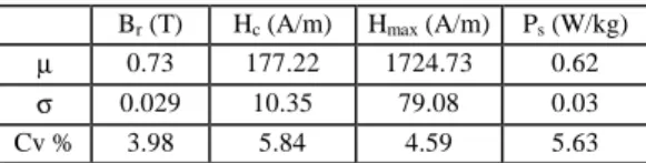
Hysteresis loops of the considered samples, measured at 5Hz and 1.5T are presented in figure 2. Moreover, the variability of the characteristics points of the hysteresis loops for the considered samples are summarized in table 1.
TABLEI
COEFFICIENT OF VARIATION OF HYSTERESIS LOOPS POINTS
Br (T) Hc (A/m) Hmax (A/m) Ps (W/kg) µ 0.73 177.22 1724.73 0.62 σ 0.029 10.35 79.08 0.03 Cv % 3.98 5.84 4.59 5.63 -2000 -1000 0 1000 2000 -1.5 -1 -0.5 0 0.5 1 1.5 H B
Figure 2: Hysteresis loops of SS samples measured at 5Hz and 1.5T
These variabilities are linked directly to the magnetic properties of the considered samples. The objective of this paper is then to develop a stochastic version of the Jiles and Atherton model to account for these variabilities.
III. STOCHASTIC MODELING APPROACH
In the literature, several papers in various fields of engineering have been concerned by the development of stochastic models for representing the behavior of a random phenomenon. A relatively vast literature dealing with such modeling can be found in the field stochastic aspect of the fatigue of materials, based on Virkler experimental data [17]. These data concerned the stochastic aspect of crack length of 68 samples, made with the same aluminium alloy and with the same dimensions. 68 individual crack growth curves, each giving the number of cycles as function of crack length, are then obtained. These observations resulted in different statistical analyzes to identify the probabilistic distribution of the input parameters of the used behavior law, as for instance the Paris and Erdogan model [16]. One can find also some works accounting for the stochastic aspect of Young’s modulus [21].
According to these works, we have defined the following steps to account for the uncertainties of the hysteretic behavior of the samples.
A. Deterministic model selection
The first step is to compare the accuracy of existing deterministic models. To this end, the objective is to identify the parameters of the deterministic model from experimental data. The coefficient of efficiency R² can be used to measure the accuracy of the fitting process. It takes values between 0 and 1, and evaluates the fraction of variance in the observed data that can be explained by the model. A higher value indicates better agreement. Assume that we have a sample of size n such as y = (y1, y2,…yn) measured at x = (x1, x2,…xn), related to the
behavior of a phenomena, and we want to estimate a family of parameters a=(a1, a2,…aq) of the model f(a)
chosen to represent the data. The least square technique can then be used to find the values of the parameters. The expression of R² is given by the following relation:
( ) ( )
(
)
( )
( )
( )
(
)
∑
∑
= = − − − = n 1 i i * i * n 1 i i i * 2 x y E x y x y x y 1 R (1)Where E(y*(xi)) is the mean over the measured points, y*(xi) and y(xi) are respectively the measured and the
point estimated by the model for the corresponding xi
level.
R² may be oversensitive to extreme values or outliers.
An improvement over R² for model evaluation purposes is the adjusted coefficient of efficiency R²a given by,
( )
2 2 a 1 R 1 q n 1 n 1 R − − − − − = (2)B. Stochastic modeling of input parameters
With the selected deterministic model, the next step consists in identifying its parameters for all experimental data. In order to verify the prediction of the stochastic model latter, one can split randomly the experimental data in two subsets: Modeling Subsets (MS) to develop the probabilistic model, and Test Subsets (TS) to test the prediction of the model. The parameters of the deterministic model are then identified on MS. The probability distribution functions (pdf) of the parameters are thereafter identified, and this can be achieved in a context of parametric approach for which classical pdf (uniform, Gaussian, lognormal) can be tested with Kolmogorov Smirnov (KS) test. In practice, the test consists in assuming that the experimental data are distributed according to the proposed pdf at a risk of α%. This assumption is known as null hypothesis H0. Then, by
computing the maximum distance between empirical Cumulative Distribution Function (CDF) of the experimental data and the CDF of the candidate distribution, one can reject or not the null hypothesis H0
at a risk of α%. The result related to the rejection or not of H0 is most of the time interpreted in term of p-value.
Therefore, one can reject H0 if the p-value returned by the
test is less than the risk α%. Moreover, and if all the proposed pdf are not rejected by the test, on can retain the
pdf that return the highest p-value. C. Correlation analysis
This step deals with the analysis of the inter-dependence between the input parameters identified in the previous step. Quantification of this dependence structure is of importance as it impacts mainly the variance of the output of the model, whereas the mean is not generally changed. The works presented in [19] stipulate that the correlation structure must be taken into account, especially when it is around 0.7.
Assume that we have a couple of random variables X1 and X2. If they are Gaussian distributed, and
only in this case, one can quantify the intensity of the dependency using the Pearson coefficient, defining a
linear intensity between both random variables. This coefficient is calculated with the following relationship:
( )
(
)
(
( )
)
[
]
2 X 1 X 2 2 1 1 p X E X X E X E r σ σ − − = (3)If both random variables are not Gaussian distributed, it may be useful to quantify the intensity of this dependence with the Spearman rank correlation [24]. This coefficient is a non parametric one, calculated from the rank of X1 and X2. In this case, the intensity of both
random variables is not necessarily linear. Moreover, if X1 and X2 are Gaussian distributed, it is as powerful as the
Pearson correlation coefficient rp and allows one to
overcome the assumption about a linear form of dependence between X1 and X2, especially for a limited
number of data.
The expression of this coefficient is given by the following relationship:
(
)
(
)
(
)
∑
(
)
∑
∑
= = = − − − − = n 1 i 2 i n 1 i 2 i i n 1 i i s S S R R S S R R ρ (4)Where Ri=Rank(xi) and Si=Rank(yi) and R and S are respectively the mean of the rank of x1 and x2.
D. Validation of the model
The validation of the model consists in performing Monte Carlo simulations, which consists simply in performing multiple model evaluations of the deterministic model, using random numbers to sample from pdf model inputs (ie sampling is guided by the pdf of each parameter). This approach is straightforward, but the main challenge of the simulation is to account for the dependency structure between the parameters. If all the parameters are then distributed according to a Gaussian distribution, a Multivariate Gaussian distribution (MGD) may be chosen to account for the marginal distribution and the correlation between them [14]. If it is not the case, Iman and Conover [24], can be implemented. This method is applicable for all type of distributions and is useful in inducing desired rank correlations among the input parameters.
The theoretical basis for the method is briefly described below [24], [25]. Suppose that [C] is a desired correlation matrix and [X] is a random row vector. Because [C] is positive-definite and symmetric, [C] may be written as [C] = [P][P’], defined as Chlosky decomposition. Then the transformed vector [X][P’] has the desired correlation matrix [C]. The detailed procedure is as follows. Let the number of input variables be denoted by k, and let n be the sample size.
Let [X] be an n×k matrix whose columns represent k independent random permutations of an arbitrary set of n scores. The usual scores, as presented in the original paper of Iman and Conover are the Van Der Waerden scores, which are generated by Φ−1{i / (n + 1)}, where Φ −1 is the inverse function of the standard normal distribution, and i = 1,..., n. For a sample of size n = 20,
the matrix [X] has a random mix of the Van Der Waerden scores Φ−1(i/21), i = 1..., 20, in each column. For k= 2, the 20 Van Der Waerden scores are independently permutated twice to create two columns of the random mix. Suppose that [C] is the desired rank correlation matrix (2×2 matrix in this case) and [C] = [P][P’], where [P] can be computed using the Cholesky factorization scheme. The Cholesky factorization factors a symmetric, positive-definite matrix [C] into the product of a lower triangular matrix [P] and its transpose [P’]. As mentioned above, [X][P’] results in an n×k matrix, denoted as [X*], which possesses the desired correlation matrix [C] for the kinput variables. Further, let [A] be an n×k matrix whose elements are actual input values (k input variables with n observations each). To induce the desired correlation between the input variables, the input values in each column of matrix [X] are rearranged to have the same ordering as the corresponding column of matrix [X*]. This method is easy to use, distribution-free (non-parametric), and preserves the exact marginal distributions of input variables.
Results of the simulation can be then used to determine the uncertainty related to the output of the model and to perform statistical analysis. It may be useful to check if the marginal distributions of each parameter are preserved and if the correlation matrix obtained with the method are close.
E. Cross Validation techniques
For the selected probabilistic model, a Cross Validation techniques (CV) is applied to analyze its prediction behavior [21]. This technique consists in identifying first a Confidence Interval CI and then by comparing the identified CI with MS and TS trajectories. The objective is then to verify if all MS lie within the identified CI. Moreover, comparison of TS and CI is also of interest as it allows one to analyze the prediction of the model. Therefore, and if all TS lie within the CI, one can imagine that the variability of over samples of stator issued form the considered production chain is inside the identified CI.
IV. HYSTERESIS LOOPS SS SAMPLES STOCHASTIC MODELING
J-A model describes, from a physical point of view the hysteresis phenomena inside soft magnetic materials. The mechanism of the original model can be consulted in [22]. In order to take account for the hysteresis variabilities among SS samples, inverse J-A model is used [30], ie, B is used as input, and given by the following relationship:
( )
( )(
)
(
)
e anh 0 e irr 0 e anh e irr dB dM 1 c dB dM 1 c 1 1 dB dM c dB dM c 1 dB dM α µ α µ − − + − + + − = (5)In this relation, Manh and Mirr denote respectively the
anhysteretic magnetization and the irreversible magnetization.
(Ms, k, c, a, α) are the parameters of the model, and
are determined from the measured hysteresis
characteristics. An identification method of the parameters is presented in [31], from some points of the hysteresis loop. However, this technique is known to be unstable numerically, and the convergence is not systematic. An improvement over the parameters identification is now available, and based especially in optimization techniques. Moreover, some works are related to the consideration of variable parameters, according to some physical observations. In [32], a variable pining parameter modeled by Gaussian function is proposed, assuming that k is higher for lower level magnitude of the applied excitation field, and lower for higher magnitude level. The expression of k is given by the following relationship:
k=k0×exp(-H²/(2×σ²) (6)
Where k0 corresponds to the original value of
parameter k, H the applied excitation field, and σ the standard deviation of the Gaussian function. The modified J-A model is then defined by 6 parameters to be identified from experimental measurements. Another variant is given in [23], when considering the same assumption. Another parameter is added, and the previous relation becomes:
k=k1+k0×exp(-H²/(2×σ²)) (7)
Where the first term is independent of the excitation field and the second term a Gaussian function. In this case, the J-A model is defined by 7 parameters.
The three models were tested on the hysteresis behavior of a sample f stator, in order to choose among the most accurate one, in term of R²a. The identified
parameters using classical least square fitting technique and the coefficient of efficiency R²afor each model are
presented in figure 2.a, 2.b and 2.c. Graphically, it can be observed that each model presents a good approximation of the data. However, and when comparing the coefficient of efficiency R²a, M1 and M2 present higher
value compared to M0. Moreover, and as M1 is only
defined by 6 parameters, it was chosen to model the hysteresis behavior of all the samples. First of all, data were splitted randomly in two subsets: 20 MS, and 8 TS. The parameters of the model M1 were then identified for
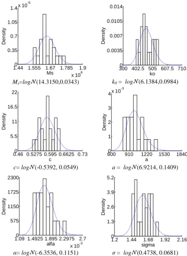
all MS. Therefore, the 6 parameters (Ms,k0,c,a,α,σ) of the
model become random but not constant anymore, and 20 realizations of the vector of parameters are obtained. Their histograms are presented in figure 3.
KS test at a risk of 5% was then performed for 3 pdf candidates, namely Gaussian, Lognormal and Uniform. The p-values returned by the test are summarized in table 2.
It can be observed in this table that the null hypothesis H0, assuming that the 6 parameters are distributed
according to the 3 candidates pdf are not rejected, at a risk of 5%. However, as the Lognormal distribution presents the highest p-value, it has been chosen to represent the variability of the 6 parameters.
The rank correlation matrix of the 6 parameters was then calculated and given in table 3. It can be observed that there is a strong correlation between them.
-2000 -1000 0 1000 2000 -1.5 -1 -0.5 0 0.5 1 1.5 Hmax [A/m] B [T ] Experimental Model -2000 -1000 0 1000 2000 -1.5 -1 -0.5 0 0.5 1 1.5 H [A/m] B [T ] Experimental Model -2000 -1000 0 1000 2000 -1.5 -1 -0.5 0 0.5 1 1.5 H [A/m] B [ T ] Experimental Model
Figure 2: Parameters and coefficient of efficiency of the three considered deterministic models
TABLEII
P-VALUES OF KOLMOGOROV SMIRNOV STATISTICAL TEST AT A RISK OF
5% OF THE 6 PARAMETERS
Ms k0 c a α σ
Gaussian 0.71 0.55 0.89 0.86 0.95 0.78 Lognormal 0.76 0.7 0.93 0.98 0.99 0.82 Uniform 0.31 0.47 0.71 0.04 0.06 0.53
In order to validate the model, Monte Carlo simulation, coupled with Iman and Conover method was performed. It was achieved by simulating independently 500,000 independent realizations of the 6 parameters according to Lognormal distribution. These realizations and the correlation matrix defined in table 3 were then used as input for Iman and Conover method. In the output of the Iman and Conover method, it was noticed that the marginal distributions for each parameter were not changed. Moreover, the disparity between the given rank correlation matrix, and the one simulated with the method was less than 1%.
1.44 1.555 1.67 1.785 1.9 x 10⁶ 0 0.35 0.7 1.05 1.4x 10 -5 Ms D e n s it y Ms=logN (14.3150,0.0343) 300 402.5 505 607.5 7100 0.0035 0.007 0.0105 0.014 ko D e n s it y k0 = logN (6.1384,0.0984) 0.46 0.5275 0.595 0.6625 0.730 5.5 11 16.5 22 c D e n s it y c= logN (-0.5392, 0.0549) 6000 910 1220 1530 1840 1 2 3 4x 10 -3 a D e n s it y a = logN (6.9214, 0.1409) 1.09 1.4925 1.895 2.2975 2.7 x 10⁻³ 0 575 1150 1725 2300 alfa D e n s it y α= logN (-6.3536, 0.1151) 1.2 1.44 1.68 1.92 2.16 0 1.3 2.6 3.9 5.2 sigma D e n s it y σ = logN (0.4738, 0.0681) Figure 3: Histograms of parameters of M1 model
TABLEIII
RANK CORRELATION MATRIX OF THE 6 PARAMETERS OF M1
Ms k0 c a Α σ Ms 1 -0.509 -0.837 0.959 0.942 0.567 k0 -0.509 1 0.746 -0.415 -0.362 -0.918 c -0.837 0.746 1 -0.787 -0.759 -0.778 a 0.959 -0.415 -0.787 1 0.99 0.516 α 0.942 -0.362 -0.759 0.992 1 0.470 σ 0.567 -0.918 -0.778 0.5162 0.470 1
The deterministic hysteresis behavior of the samples was then simulated 500,000 times with the random parameters. For the 4 characteristic points of hysteresis, KS test was performed at a risk of 5% and the p-values returned by the test are summarized in table 4. Therefore, and at risk of 5%, the null hypothesis related to the equality of the distributions of the experimental data and the simulated one is not rejected, for the 4 characteristic points.
The medians of the 4 hysteresis characteristic points are then identified and presented in table 5. It can be observed that they are close
TABLE IV
P-VALUES OF KOLMOGOROV SMIRNOV KS STATISTICAL FOR THE 4
HYSTERESIS CHARACTERISTIC POINTS
Br Hc Hmax Ptot p-values 0.42 0.078 0.53 0.21 Ms =1727481.13 k = 386.53 c = 0.55 a = 1175.61 α = 0.0019 R²a= 0.93 Ms = 1696792.45 k0 = 434.50 σ = 1.67 c = 0.54 a = 1135.67 α = 0.0019 R²a= 0.97 Ms =1717876.52 k1 = 189 k0 = 247.11 σ = 0.99 c = 0.54 a = 1203 α = 0.0020 R²a= 0.97
TABLE V
EXPERIMENTAL AND SIMULATED MEDIANS OF THE CHARACTERISTIC POINTS OF HYSTERESIS Br Hc Hmax Ptot Experimental median 0.740 180.78 1702 0.627 Simulated median 0.734 176.31 1726.6 0.619 Disparity % 0.87% 2.4% 1.3% 1.24%
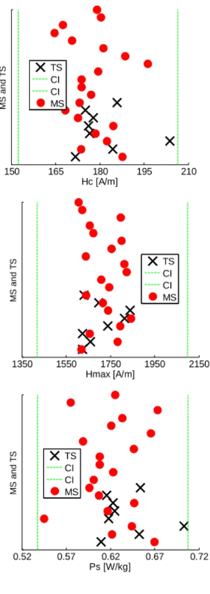
Finally 95% CI is identified, as summarized in table 6, and compared with MS and TS. These comparisons are presented in figure 4.
TABLEVI
CONFIDENCE INTERVALS IDENTIFIED FROM THE STOCHASTIC MODEL
Br (T) [0.6355; 0.8161]
Hc (A/m) [157.58; 205.13]
Hmax (A/m) [1595.29; 1842.13]
Ps (W/kg) [0.542; 0.717]
It can be observed that MS and TS lie within the 95% identified CI. All these criteria allow then one to validate the hysteresis stochastic developed model, and its prediction behavior.
V. CONCLUSION
In this paper, a stochastic modeling of the quasi-static hysteresis of 28 SS samples is developed using the J-A model. The samples are issued from a production chain, and showed variability in term of hysteresis iron losses. This variability reflects the non uniformity of the deterioration of the magnetic properties, introduced by the manufacturing process. The stochastic modeling approach was then defined, by means of existing works. Moreover, the dependency structure was considered using Iman and Conover method. The model was finally validated using statistical test and Cross Validation Techniques, and showed good results. The developed model can be used for finite element simulations. However, and in order to minimize the numerical time consumption, it may be is suitable to develop model to account for the dependency structure between parameters. In this case, polynomial chaos expansion and copula technique may be used.
0.55 0.6325 0.715 0.7975 0.88 Br [T] M S a n d T S TS CI CI MS 150 165 180 195 210 Hc [A/m] M S a n d T S TS CI CI MS 1350 1550 1750 1950 2150 Hmax [A/m] M S a n d T S TS CI CI MS 0.52 0.57 0.62 0.67 0.72 Ps [W/kg] M S a n d T S TS CI CI MS REFERENCES
[1] E.Dlala, A.Belahcen, A.Arkkio, “On the Importance of Incorporating Iron Losses in the Magnetic Field Solution of Electrical Machines”, IEEE Trans on Mag. Vol. 46, N°8, pp 3101-3104, 2010.
[2] K.Yamazaki, N.Fukushima, « Iron-Loss Modeling for Rotating Machines: Comparison Between Bertotti’s Three-Term Expression and 3-D Eddy-Current Analysis”, IEEE Trans on Mag. Vol. 46, N°8 , pp 3121-3124, 2010.
[3] C.Simão, N. Sadowski, N. J. Batistela, J. P. A. Bastos, “Evaluation of Hysteresis Losses in Iron Sheets Under DC-biased Inductions”, IEEE Trans on Mag. Vol. 45, N°3 , pp 1158-1161, 2009.
[4] J.Korecki, A.Benabou, Y.Le Menach, F.Piriou, J.P.Ducreux, “Hysteresis Phenomenon Implementation in FIT: Validation With Measurements”, IEEE Trans on Mag. Vol. 46, N°8 , pp 3286-3289, 2010.
[5] A. Boglietti, A. Cavagnino, M. Lazzari, and M. Pastorelli, “Effects of punch process on the magnetic and energetic properties of soft magnetic material,” in Proc. Electric Machines and Drives Conf., IEMDC, pp. 396–399, 2001
[6] M.Emura, F.J.G Landgraf, W.Ross and and J.R Barretta, “Influence of cutting techniques on the magnetic properties of electrical steels”, Journal of Magnetism and Magnetic Materials, 254-255, pp.358-360, 2003
[7] L.Vandenbossch, S.Jacobs, F.Henrotte and K.Hameyer “Impact of cut edges on magnetization curves and iron losses in e-machines for automotive traction” , The 25th World Battery, Hybrid and Fuel Cell Electric Vehicle Symposium & Exhibition, 2010
[8] A.Schoppa, J.Schneider, C-D Wuppermann, T.Bakon, “Influence of welding and sticking of laminations on the magnetic properties of non oriented electrical steel”, Journal of Magnetism and Magnetic Materials, 254-255, pp.367-369, 2003
[9] A.Peksoz, S.Erdem, N.Derebasi, “Mathematical model for cutting effect on magnetic flux distribution near the cut edge of non-oriented electrical steels”, Computational Materials Science, Vol.43, pp.1066–1068, 2008.
[10] F.Ossart, E.Hug, O.Hubert, C.Buvat, and R. Billardon, “Effect of Punching on Electrical Steels: Experimental and Numerical Coupled Analysis”, in IEEE Trans.Mag. Vol.36, No. 5, pp 3137-3140, 2000.
[11] F.Libert, J.Soulard, “Manufacturing Methods of Stator Cores with Concentrated Windings”, Proceedings of IET International Conference on Power Electronics, Machines and Drives PEMD, pp. 676-680, 2006.
[12] R.Ramarotafika, A. Benabou, S. Clénet, J.C. Mipo, “Experimental Characterization of the Iron Losses Variability in Stators of Electrical Machines”, in IEEE Trans. Mag., Vol. 48, no. 4, pp. 1629–1632, 2012.
[13] K.Beddek, Y.Le Menach, S.Clénet, O.Moreau, "3D stochastic Spectral Finite Element Method in static electromagnetism using vector potential formulation", IEEE Trans. Mag.,Vol. 47, N°. 5, pp.1250-1253, 5-2011
[14] R.Ramarotafika, A.Benabou, S.Clénet, "Stochastic Modeling of Soft Magnetic Properties of Electrical Steels: Application to Stators of Electrical Machines", IEEE Trans.Mag., Vol. 48, N°. 10, pp. 2573 - 2584, 10-2012
[15] D.H.Mac, S.Clénet, J.C.Mipo, O.Moreau, "Solution of Static Field Problems with Random Domains", IEEE Trans.Mag., Vol. 46, N°. 8, pp.3385-3388, 8-2010
[16] P.Paris, F.Erdogan, "A critical analysis of crack propagation laws", Journal of Basic Engineering, Vol.85, Issue 4, pp 528– 534, 1963
[17] D. A.Virkler, B. M. Hillberry, et P. K. Goel, "The statistical nature of fatigue crack propagation", Journal of Engineering Materials and Technology, Vol.101, Issue 2, pp148-153, 1979
[18] O. Ditlevsen, R.Olesen, "Statistical analysis of the Virkler data on fatigue crack growth", Engineerrng Fracture Mechanics, Vol. 25. No. 2, pp. 177-195, 1986
[19] W. Shen, A.B.O. Soboyejo,W.O. Soboyejo, "Probabilistic modeling of fatigue crack growth in Ti–6Al–4V", International journal of fatigue, Vol 23, Issue 10, pp 917-925, 2001
[20] Z. A.Kotulski, "On efficiency of identification of a stochastic crack propagation model based on Virkler experimental data", Archives of Mechanics, Vol.50, Issue 5, pp .829-847, 1998 [21] Mehrez, A. Doostan, D. Moens, D. Vandepitte, "A Validation
Study of a Stochastic Representation of Composite Material Properties from Limited Experimental Data", Proceedings of ISMA, 2010
[22] D.C. Jiles and J.L. Atherton, "Theory of ferromagnetic hysteresis",in J. Magn. Magn. Mater, Vol. 61, pp. 48-60, 1986. [23] M. Toman, G. Stumberger, D. Dolinar,“Parameter Identification
of the Jiles–Atherton Hysteresis Model Using Differential Evolution”, in IEEE Trans.Mag. Vol.44, No. 6, pp 1098-1101, 2008.
[24] R. L. Iman and W. J. Conover. "distribution-free approach to inducing rank correlation among input variables", in
Communications in Statistics B11(3), pp 311-334, 1982.
[25] F.C.Wu , Y.P.Tsang, “Second-order Monte Carlo uncertainty/variability analysis using correlated model parameters: application to salmonid embryo survival risk assessment”, Ecological Modelling Vol. 177, pp 393-414, 2004 [26] X.-C. Zhang, "Generating correlative storm variables for cligen
using a distribution free approach", Transactions of the ASAE, Vol. 48(2): 567−575, 2005
[27] L. Mehrez1, A. Doostan, D. Moens, D. Vandepitte, “A Validation Study of a Stochastic Representation of Composite Material Properties from Limited Experimental Data”, Proceedings of ISMA 2010-USD 2010, K.U.Leuven, Department Mechanical Engineering, 2010.
[28] E.Etien, D.Halbert, and T.Poinot, “Improved Jiles–Atherton Model for Least Square Identification Using Sensitivity Function Normalization”, IEEE Trans on Mag. Vol. 44, N°7, pp 1721-1727, 2008.
[29] D.Miljaveca, B.Zidaric, « Introducing a domain flexing function in the Jiles– Atherton hysteresis model”, Journal of Magnetism
and Magnetic Material 320, pp.763-768, 2008.
[30] N. Sadowski, N. J. Batistela, J. P. A. Bastos, and M. Lajoie-Mazenc, “An Inverse Jiles–Atherton Model to Take Into Account
Hysteresis in Time-Stepping Finite-Element Calculations”, IEEE Trans.Mag., Vol. 38, N°. 2, pp. 797 -800, 03-2002
[31] D.C. Jiles, J. B. Thoelke. and M. K. Devine, “ Numerical Determination of Hysteresis Parameters the Modeling of Magnetic Properties Using the Theory of Ferromagnetic Hysteresis”, in IEEE Trans.Mag. Vol.28, No. 1, pp27-35, 1992. [32] P.R.Wilson, J.N.Ross, A.D.Brown, “Optimizing the Jiles-Atherton
model of hysteresis by a genetic algorithm”, IEEE Trans.Mag. Vol. 37, No 2, pp 989-993, 2002