Science Arts & Métiers (SAM)
is an open access repository that collects the work of Arts et Métiers Institute of
Technology researchers and makes it freely available over the web where possible.
This is an author-deposited version published in: https://sam.ensam.eu
Handle ID: .http://hdl.handle.net/10985/6784
To cite this version :
Florent RAVELET, René DELFOS, Jerry WESTERWEEL - Influence of global rotation and Reynolds number on the large-scale features of a turbulent Taylor–Couette flow - PHYSICS OF FLUIDS p.1-8 - 2010
Any correspondence concerning this service should be sent to the repository Administrator : archiveouverte@ensam.eu
We experimentally study the turbulent flow between two coaxial and independently rotating cylinders. We determined the scaling of the torque with Reynolds numbers at various angular velocity ratios 共Rotation numbers兲 and the behavior of the wall shear stress when varying the Rotation number at high Reynolds numbers. We compare the curves with particle image velocimetry analysis of the mean flow and show the peculiar role of perfect counter-rotation for the emergence of organized large scale structures in the mean part of this very turbulent flow that appear in a smooth and continuous way: the transition resembles a supercritical bifurcation of the secondary mean flow. © 2010 American Institute of Physics. 关doi:10.1063/1.3392773兴
I. INTRODUCTION
Turbulent shear flows are present in many applied and fundamental problems, ranging from small scales共such as in the cardiovascular system兲 to very large scales 共such as in meteorology兲. One of the several open questions is the emer-gence of coherent large-scale structures in turbulent flows.1 Another interesting problem concerns bifurcations, i.e., tran-sitions in large-scale flow patterns under parametric influ-ence, such as laminar-turbulent flow transition in pipes, or flow pattern change within the turbulent regime, such as the dynamo instability of a magnetic field in a conducting fluid,2 or multistability of the mean flow in von Kármán or free-surface Taylor–Couette flows,3,4leading to hysteresis or non-trivial dynamics at large scale. In flow simulation of homo-geneous turbulent shear flow it is observed that there is an important role for what is called the background rotation, which is the rotation of the frame of reference in which the shear flow occurs. This background rotation can both sup-press or enhance the turbulence.5,6 We will further explicit this in Sec. III.
A flow geometry that can generate both motions—shear and background rotation—at the same time is the Taylor– Couette flow which is the flow produced between differen-tially rotating coaxial cylinders.7When only the inner cylin-der rotates, the first instability, i.e., deviation from laminar flow with circular streamlines, takes the form of toroidal 共Taylor兲 vortices. With two independently rotating cylinders, there is a host of interesting secondary bifurcations, exten-sively studied at intermediate Reynolds numbers, following the work of Coles8and Andereck et al.9Moreover, it shares strong analogies with Rayleigh–Bénard convection,10,11 which are useful to explain different torque scalings at high Reynolds numbers.12,13Finally, for some parameters relevant in astrophysical problems, the basic flow is linearly stable and can directly transit to turbulence at a sufficiently high Reynolds number.14
The structure of the Taylor–Couette flow, while it is in a
turbulent state, is not so well known and only few
measure-ments are available.15 The flow measurements reported in Ref. 15and other torque scaling studies only deal with the case where only the inner cylinder rotates.12,13In that precise case, recent direct numerical simulations suggest that vortexlike structures still exist at high Reynolds number 共Reⲏ104兲,16,17
whereas for counter-rotating cylinders, the flows at Reynolds numbers around 5000 are identified as “featureless states.”9The structure of the flow is exemplified with a flow visualization in Fig.1in our experimental setup for a flow with only the inner cylinder rotating, counter-rotating cylinders, and only the outer cylinder counter-rotating, respectively.
In the present paper, we extend the study of torques and flow field for independently rotating cylinders to higher Reynolds numbers 共up to 105兲 and address the question of
the transition process between a turbulent flow with Taylor vortices, and this “featureless” turbulent flow when varying the global rotation while maintaining a constant mean shear rate.
In Sec. II, we present the experimental device and the measured quantities. In Sec. III, we introduce the specific set of parameters we use to take into account the global rotation through a “Rotation number” and the imposed shear through a shear-Reynolds number. We then present torque scalings and typical velocity profiles in turbulent regimes for three particular Rotation numbers in Sec. IV. We explore the tran-sition between these regimes at high Reynolds number vary-ing the Rotation number in Sec. V and discuss the results in Sec. VI.
II. EXPERIMENTAL SETUP AND MEASUREMENT TECHNIQUES
The flow is generated between two coaxial cylinders 共Fig. 2兲. The inner cylinder has a radius of ri= 110
⫾0.05 mm and the outer cylinder of ro= 120⫾0.05 mm.
The gap between the cylinders is thus d = ro− ri= 10 mm and
a兲Electronic mail: florent.ravelet@ensta.org.
the gap ratio is= ri/ro= 0.917. The system is closed at both
ends, with top and bottom lids rotating with the outer cylin-der. The length of the inner cylinder is L = 220 mm 共axial aspect ratio is L/d=22兲. Both cylinders can rotate indepen-dently with the use of two dc motors共Maxon, 250 W兲. The motors are driven by a homemade regulation device, ensur-ing a rotation rate up to 10 Hz, with an absolute precision of ⫾0.02 Hz and a good stability. ALABVIEW program is used to control the experiment: the two cylinders are simulta-neously accelerated or decelerated to the desired rotation rates, keeping their ratio constant. This ratio can also be changed while the cylinders rotate, maintaining a constant differential velocity.
The torque T on the inner cylinder is measured with a corotating torque meter共HBM T20WN, 2 N m兲. The signal is recorded with a 12 bit data acquisition board at a sample rate of 2 kHz for 180 s. The absolute precision on the torque measurements is⫾0.01 N m, and values below 0.05 N m are rejected. We also use the encoder on the shaft of the torque meter to record the rotation rate of the inner cylinder. Since that matches excellently with the demanded rate of rotation, we assume that the outer cylinder rotates at the demanded rate as well.
Since the torque meter is mounted in the shaft between driving motor and cylinder, it also records 共besides the in-tended torque on the wall bounding the gap between the two cylinders兲 the contribution of mechanical friction such as in the two bearings, and the fluid friction in the horizontal 共Kármán兲 gaps between tank bottom and tank top. While the bearing friction is considered to be marginal共and measured
so in an empty, i.e., air filled system兲, the Kármán-gap con-tribution is much bigger: during laminar flow, we calculated and measured this to be of the order of 80% of the gap torque. Therefore, all measured torques were divided by a factor of 2, and we should consider the scaling of torque with the parameters defined in Sec. III as more accurate than the exact numerical values of torque.
A constructionally more difficult, but also more accurate, solution for the torque measurement is to work with three stacked inner cylinders and only measure the torque on the central section, such as is done in the Maryland Taylor– Couette setup,12 and 共under development兲 in the Twente Turbulent Taylor–Couette setup.18
We measure the three components of the velocity by stereoscopic particle image velocimetry 共PIV兲19 in a plane illuminated by a double-pulsed Nd:yttrium aluminum garnet laser. The plane is vertical共Fig.2兲, i.e., normal to the mean
flow: the in-plane components are the radial共u兲 and axial 共v兲 velocities, while the out-of-plane component is the azimuthal component共w兲. It is observed from both sides with an angle of 60°共in air兲 using two double-frame charge coupled device cameras on Scheimpflug mounts. The light-sheet thickness is 0.5 mm. The tracer particles are 20 m fluorescent 共rhodamine B兲 spheres. The field of view is 11⫻25 mm2,
corresponding to a resolution of 300⫻1024 pixels. Special care has been taken concerning the calibration procedure, on which especially the evaluation of the plane-normal azi-muthal component heavily relies. As a calibration target we use a thin polyester sheet with lithographically printed crosses on it, stably attached to a rotating and translating microtraverse. It is first put into the light sheet and traversed perpendicularly to it. Typically, five calibration images are taken with intervals of 0.5 mm. The raw PIV images are processed usingDAVIS 7.2by Lavision. They are first mapped to world coordinates, then they are filtered with a min-max filter, then PIV processed using a multipass algorithm, with a last interrogation area of 32⫻32 pixels with 50% overlap, and normalized using median filtering as postprocessing. Then, the three components are reconstructed from the two camera views. The mapping function is a third-order polyno-mial, and the interpolations are bilinear. The PIV data acqui-sition is triggered with the outer cylinder when it rotates in order to take the pictures at the same angular position as used during the calibration.
FIG. 1. Photographs of the flow at Re= 3.6⫻103. Left, A: only the inner cylinder rotating. Middle, B: counter-rotating cylinders. Right, C: only the outer cylinder rotating. The flow structure is visualized using microscopic mica platelets共Pearlessence兲.
ω ω r = 120 mm o i o r = 110 mmi h = 220 mm PIV plane 1.5 mm (b) (a)
FIG. 2. Picture and sketch with dimensions of the experimental setup. One can see the rotating torque meter共upper part of the picture兲, the calibration grid displacement device共on top of the upper plate兲, one of the two cameras 共left side兲, and the light sheet arrangement 共right side兲. The second camera is further to the right.
To check the reliability of the stereoscopic velocity measurement method, we performed a measurement for a laminar flow when only the inner cylinder rotates at a Reynolds number as low as ReS= 90 using an 86%
glycerol-water mixture. In that case, the analytical velocity field is known: the radial and axial velocities are zero, and the azi-muthal velocity w should be axisymmetric with no axial de-pendence, and a radial profile in the form w共r兲=⍀ri共ro/r
− r/ro兲/共1−2兲. 8
The results are plotted in Fig.3. The mea-sured profile 共solid line兲 hardly differs from the theoretical profile共dashed line兲 in the bulk of the flow 关0.1ⱗ共r−ri兲/d
ⱗ0.7兴. The discrepancy is, however, quite strong close to the outer cylinder关共r−ri兲/d=1兴, which may be due to the
refrac-tion close to the curved wall that causes measurement errors. The in-plane components, which should be zero, do not ex-ceed 1% of the inner cylinder velocity everywhere. In con-clusion, the measurements are very satisfying in the bulk. Further improvements to the technique have been made since this first PIV test, in particular a new outer cylinder of im-proved roundness, and the measurements performed in water for turbulent cases are reliable in the range 关0.1ⱗ共r−ri兲/d
ⱗ0.85兴. The PIV measurements close to the wall could be further improved by using an outer cylinder that is machined in a block with flat outer interfaces normal to the cameras.
III. PARAMETER SPACE
The two traditional parameters to describe the flow are the inner 共respectively, outer兲 Reynolds numbers Rei
=共riid/兲 关respectively, Reo=共rood/兲兴, with the inner
共respectively, outer兲 cylinder rotating at rotation ratesi
共re-spectively,o兲, and the kinematic viscosity.
We choose to use the set of parameters defined by Du-brulle et al.:20a shear Reynolds number ReSand a Rotation
number Ro, ReS= 2兩Reo− Rei兩 1 + Ro =共1 −兲 Rei+ Reo Reo− Rei . 共1兲
With this choice, ReS is based on the laminar shear rate
S: ReS= Sd2/. For instance, with a 20 Hz velocity difference
共rii= −roo兲. Two other relevant values of the Rotation
number are Roi=− 1⯝−0.083 and Roo=共1−兲/⯝0.091
for, respectively, inner and outer cylinders rotating alone. Finally, a further choice that we made in our experiment was the value of = ri/ro, which we have chosen as relatively
close to unity, i.e.,= 110/120⯝0.91, which is considered a narrow gap, and is the most common in reported experi-ments, such as Refs.8,9,21, and22, although a value as low as 0.128 is described as well.4A high, i.e.,共1−兲Ⰶ1, is special in the sense that for→1 the flow is equivalent to a plane Couette flow with background rotation; at high, the flow is linearly unstable for −1⬍Ro⬍Roo.5,20,23
In the present study we experimentally explore regions of the parameter space that, to our knowledge, have not been reported before. We present in Fig.4the parameter space in 兵Reo; Rei其 coordinates with a sketch of the flow states
iden-tified by Andereck et al.9 and the location of the data dis-cussed in the present paper. One can notice that the present range of Reynolds numbers is far beyond that of Andereck, and that with the PIV data we mainly explore the zone be-tween perfect counter-rotation and only the inner cylinder rotating.
IV. STUDY OF THREE PARTICULAR ROTATION NUMBERS
In the experiments reported in this section, we maintain the Rotation number at constant values and vary the shear Reynolds number. We compare three particular Rotation numbers, Roi, Roc, and Roo, corresponding to rotation of the
inner cylinder only, exact counter-rotation, and rotation of the outer cylinder rotating only, respectively. In Sec. IV A, we report torque scaling measurements for a wide range of Reynolds numbers—from base laminar flow to highly turbu-lent flows—and in Sec. IV B, we present typical velocity profiles in turbulent conditions.
A. Torque scaling measurements
We present in Fig. 5 the friction factor cf
= T/共2ri2LU2兲⬀G/Re2, with U = Sd and G = T/共L2兲, as a
function of ReS for the three Rotation numbers. A common
definition for the scaling exponent ␣ of the dimensionless torque is based on G: G⬀ReS␣. We keep this definition and
present the local exponent ␣ in the inset in Fig. 5. We compute ␣ by means of a logarithmic derivative, ␣= 2 + d log共cf兲/d log共ReS兲.
At low Re, the three curves collapse on a Re−1 curve.
This characterizes the laminar regime where the torque is proportional to the shear rate on which the Reynolds number is based.
0 .2 .4 .6 .8 1
0
(r−ri)/d
FIG. 3. Dimensionless azimuthal velocity profile关w/共rii兲 vs 共r−ri兲/d兴 for Ro= Roiat ReS= 90共see Sec. III for the definition of the parameters兲. Solid line: measured mean azimuthal velocity. Dashed line: theoretical profile. The radial component u, which should be zero, is also shown as a thin solid line.
FIG. 4.共Color online兲 Parameter space in 兵Reo; Rei其 coordinates. The vertical axis Reo= 0 corresponds to Ro= Roi= −0.083 and has been widely studied共Refs.
12,13,16, and17兲. The horizontal axis Rei= 0 corresponds to Ro= Roo= 0.091. The line Rei= −Reocorresponds to counter-rotation, i.e., Ro= Roc= 0. The PIV data taken at a constant shear Reynolds number of ReS= 1.4⫻104are plotted with共䊊兲. The torque data with varying Ro at constant shear for various ReS ranging from ReS= 3⫻103to ReS= 4.7⫻104are plotted as gray共blue online兲 lines. They are discussed in Fig.8. We also plot the states identified at much lower ReSby Andereck et al.共Ref.9兲 as patches: black corresponds to laminar Couette flow, gray 共green online兲 to “spiral turbulence,” dotted zone to “featureless turbulence,” and vertical stripes to an “unexplored” zone.
101 102 103 104 105 106 10−3 10−2 10−1 Re C f 101 102 103 104 105 106 1 1.5 2 Re α
FIG. 5.共Color online兲 Friction factor cfvs ReSfor Roi=− 1共black 䊊兲, Roc= 0共blue 䊐兲, and Roo=共1−兲/共red 〫兲. Relative error on ReS:⫾5%; absolute error on torque:⫾0.01 N m. Dashed 共green online兲 line: Lewis’ data 关Ref.13, Eq.共3兲兴, for Roiand= 0.724. Dash-dotted共magenta online兲 line: Racina’s data 关Ref. 22, Eq. 共10兲兴. Solid thin black line: laminar friction factor cf= 1/共Re兲. Inset: local exponent ␣ such that Cf⬀ReS␣−2, computed as 2 + d log共Cf兲/d log共ReS兲, for Roi=− 1共black 䊊兲, Roc= 0共blue 䊐兲, and Roo=共1−兲/共red 〫兲. Dashed 共green online兲 line: Lewis’ data 关Ref.13, Eq.共3兲兴 for Roiand= 0.724.
than the theoretical prediction Recc= 515,23 which is
prob-ably due to our finite aspect ratio. Finally, the Taylor–Couette flow with only the outer cylinder rotating关Roo=共1−兲/兴 is
linearly stable whatever Re. We observe the experimental flow to be still laminar up to high Re; then, in a rather short range of Re numbers, the flow transits to a turbulent state at 4000ⱗReto⯝5000.
Further increase in the shear Reynolds number also increases the local exponent 共see inset in Fig. 5兲. For
Roi=− 1, it gradually rises from ␣⯝1.5 at Re⯝200 to
␣⯝1.8 at Re⯝105. The order of magnitude of these values
agrees with the results of Lewis et al.,13 although a direct comparison is difficult, owing to the different gap ratios of the experiments. The local exponent is supposed to approach a value of 2 for increasing gap ratio. Dubrulle and Hersant10 attribute the increase in␣to logarithmic corrections, whereas Eckhardt et al.11attribute the increase in ␣to a balance be-tween a boundary-layer/hairpin contribution 共scaling as ⬀Re3/2兲 and a bulk contribution 共scaling as ⬀Re2兲. The
case of perfect counter-rotation shows a plateau at ␣⯝1.5 and a sharp increase in the local exponent to ␣⯝1.75 at Retc⯝3200, possibly tracing back to a secondary transition.
The local exponent then seems to increase gradually. Finally, for outer cylinder rotating alone共Roo兲 the transition is very
sharp and the local exponent is already around ␣= 1.77 at Reⲏ5000. Note that the dimensional values of the torque at Roo are very small and difficult to measure accurately, and
that these may become smaller than the contributions by the two Kármán layers 共end effects兲 that we simply take into account by dividing by 2, as described in Sec. II. One can finally notice that at the same shear Reynolds number, for Reⱖ104 the local exponents for the three rotation numbers
are equal within ⫾0.1 and that the torque with the inner cylinder rotating only is greater than the torque in counter-rotation, the latter being greater than the torque for only the outer cylinder rotating.
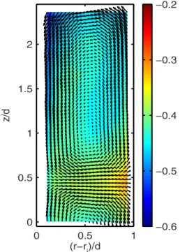
B. Velocity profiles at a high shear-Reynolds number The presence of vortexlike structures at high shear-Reynolds number 共ReSⲏ104兲 in turbulent Taylor–Couette
flow with the inner cylinder rotating alone is confirmed in our experiment through stereoscopic PIV measurements.24 As shown in Fig.6, the time-averaged flow shows a strong secondary mean flow in the form of counter-rotating vorti-ces, and their role in advecting angular momentum共as ible in the coloring by the azimuthal velocity兲 is clearly vis-ible as well. The azimuthal velocity profile averaged over both time and axial position w, as shown in Fig.7, is almost flat, indicating that the transport of angular momentum is due
mainly to the time-average coherent structures rather than by the correlated fluctuations as in regular shear flow.
We then measured the counter-rotating flow at the same ReS. The measurements are triggered on the outer cylinder
position and are averaged over 500 images. In the counter-rotating case, for this large gap ratio and at this value of the shear-Reynolds number, the instantaneous velocity field is really disorganized and does not contain obvious structures like Taylor vortices, in contrast with other situations.25 No peaks are present in the time spectra, and there is no axial dependency of the time-averaged velocity field. We thus av-erage in the axial direction the different radial profiles; the
0 0.5 1 0 0.5 1 (r−r i)/d z/ d −0.6 −0.5 −0.4
FIG. 6.共Color online兲 Secondary flow for Ro=Roiat Re= 1.4⫻104. Arrows indicate radial and axial velocities; color indicates azimuthal velocity 共nor-malized to inner wall velocity兲.
0 0.2 0.4 0.6 0.8 1 −1 −0.8 −0.6 −0.4 −0.2 0 0.2 0.4 0.6 0.8 1 Velocity (dimless ) (r−ri)/d Ro i Ro o Ro c
FIG. 7.共Color online兲 Profiles of the mean azimuthal velocity component for three Rotation numbers corresponding to only the inner cylinder rotating 共⫻, black兲, perfect counter-rotation 共䊊, blue兲, and only the outer cylinder rotating共쐓, red兲 at Re=1.4⫻104. Thin line共·, black兲: axial velocity v 共for Ro= Roi兲 averaged over half a period. The velocities are presented in a dimensionless form: w/共Sd兲 with Sd=2ri共o−i兲/共1+兲.
azimuthal component w is presented in Fig.7as well. In the bulk, it is low, i.e., its magnitude is below 0.1 between 0.15ⱗ共r−ri兲/dⱗ0.85, that is 75% of the gap width. The
two other components are zero within 0.002.
We finally address the outer cylinder rotating alone again at the same ReS. These measurements are done much in the
same way as the counter-rotating ones, i.e., again the PIV system is triggered by the outer cylinder. As in the counter-rotating flow, this flow does not show any large scale struc-tures. The gradient in the average azimuthal velocity, again shown in Fig.7, is much steeper than in the counter-rotating case, which can be attributed to the much lower turbulence, as it also manifests itself in the low cfvalue for Roo.
V. INFLUENCE OF ROTATION ON THE EMERGENCE AND STRUCTURE OF THE TURBULENT
TAYLOR VORTICES
To characterize the transition between the three flow re-gimes, we first consider the global torque measurements. We plot in Fig.8the friction factor or dimensionless torque as a function of Rotation number Ro at six different shear Reynolds numbers ReS, as indicated in Fig.4. We show three
series centered around ReS= 1.4⫻104 and three around
ReS= 3.8⫻104. As already seen in Fig.5, the friction factor
reduces with increasing ReS. More interesting is the behavior
of cfwith Ro: the torque in counter-rotation共Roc兲 is
approxi-mately 80% of cf共Roi兲, and the torque with outer cylinder
rotating alone共Roo兲 is approximately 50% of cf共Roi兲. These
values compare well with the few available data compiled by Dubrulle et al.20 The curve shows a plateau of constant torque especially at the larger ReS from Ro= −0.2, i.e.,
when both cylinders rotate in the same direction with the inner cylinder rotating faster than the outer cylinder, to Ro⯝−0.035, i.e., with a small amount of counter-rotation with the inner cylinder still rotating faster than the outer cylinder. The torque then monotonically decreases when in-creasing the angular speed of the outer cylinder, with an inflexion point close or equal to Roc. It is observed that the
transition is continuous and smooth everywhere and without hysteresis.
We now address the question of the transition between the different torque regimes by considering the changes ob-served in the mean flow. To extract quantitative data from the PIV measurements, we use the following model for the stream function⌿ of the secondary flow:
⌿ = sin
冉
共r − ri兲 d冊
⫻冋
A1sin冉
共z − z0兲 ᐉ冊
+ A3sin冉
3共z − z0兲 ᐉ冊
册
, 共2兲with as free parameters A1, A3,ᐉ and z0. This model com-prises a flow that fulfills the kinematic boundary condition at the inner and outer walls, ri, ri+ d, and in between forms in
the axial direction alternating rolls, with a roll height ofᐉ. In this model, the maximum radial velocity is formed by the two amplitudes and given by ur,max=共⌿/z兲max=共A1/ᐉ
+ 3A3/ᐉ兲. It is implicitly assumed that the flow is developed sufficiently to restore the axisymmetry, which is checked
a posteriori. Our fitting model comprises a sinusoidal
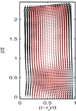
共fun-damental兲 mode and its first symmetric harmonic 共third mode兲, the latter which appears to considerably improve the matching between the model and the actual average velocity fields, especially close to Roi共see Figs.9 and10兲.
We first discuss the case Ro= Roi. A sequence of 4000
PIV images at a data rate of 3.7 Hz is taken, and 20 consecu-tive PIV images, i.e., approximately 11 cylinder revolutions, are sufficient to obtain a reliable estimate of the mean flow.17 It is known that for the first transition the observed flow state can depend on the initial conditions.8When starting the inner cylinder from rest and accelerating it to 2 Hz in 20 s, the vortices grow very fast, reach a value with a velocity ampli-tude of 0.08 ms−1, and then decay to become stabilized at a
−0.1 −0.05 0 0.05 0.1 0 0.2 0.4 0.6 0.8 1.0 1.2 1.4 1.6 1.8 2.0 2.2 Ro 10 3 × Cf Roi Roc Roo
FIG. 8.共Color online兲 The friction factor cfas a function of Ro at various constant shear Reynolds numbers: 共blue 䊐兲 Re=1.1⫻104, 共red 〫兲 Re = 1.4⫻104,共green 䊊兲 Re=1.7⫻104,共black 쐓兲 Re=2.9⫻104,共magenta ⫻兲 Re= 3.6⫻104,共cyan 䉮兲 Re=4.7⫻104.
0 0.5 1 0 0.5 1 1.5 2 (r−r i)/d
z/
d
FIG. 9.共Color online兲 Overlay of measured time-average velocity field at Ro= Roi 关in gray 共red online兲兴 and the best-fit model velocity field 共in black兲. The large third harmonic makes the radial flow being concentrated in narrow bands rather than sinusoidally distributed.
value around 0.074 ms−1after 400 s. Transients are thus also
very long in turbulent Taylor-vortex flows. For slower accel-eration, the vortices that appear first are much weaker and have a larger length scale before reaching the same final state. The final length scaleᐉ of the vortices for Roiis about
1.2 times the gap width, consistent with the data from Bilson
et al.16
In a subsequent measurement we start from Ro= Roiand
vary the rotation number in small increments, while main-taining a constant shear rate. We allow the system to spend 20 min in each state before acquiring PIV data. We verify that the fit parameters are stationary and compute them using the average of the full PIV data set at each Ro. The results are plotted in Fig.10. Please note that Ro has been varied both with increasing and decreasing values to check for a possible hysteresis. All points fall on a single curve; the tran-sition is smooth and without hysteresis. For Roⱖ0, the fitted modes have zero or negligible amplitudes, since there are no structures in the time-average field.24One can notice that as soon as Ro⬍0, i.e., as soon as the inner cylinder wall starts to rotate faster than the outer cylinder wall, vortices begin to grow. We plot in Fig. 10 the velocity amplitude associated with the simple model共single mode, 〫兲 and with the com-plete model 共modes 1 and 3, 䊊兲. Close to Ro=0, the two models coincide: A3⯝0 and the mean secondary flow is well described by pure sinusoidal structures. For Roⱗ−0.04, the vortices start to have elongated shapes with large cores and small regions of large radial motions in between adjacent vortices; the third mode is then necessary to adequately de-scribe the secondary flow共Fig.9兲. The first mode becomes
saturated共i.e., it does not grow in magnitude兲 in this region. Finally, we give in Fig.10 a fit of the amplitudes close to Ro= 0 of the form A = a共−Ro兲1/2. The velocity amplitude of
the vortex behaves like the square root of the distance to Ro= 0, a situation reminiscent to a classical supercritical bi-furcation, with A as order parameter and Ro as control parameter.
We also performed a continuous transient experiment, in which we varied the rotation number quasistatically from Ro= 0.004 to Ro= −0.0250 in 3000 s, always keeping the
very long time-averaged series leads to well-established sta-tionary axisymmetric states, it is possible that the instanta-neous whole flow consists of different regions. Further investigation including time-resolved single-point measure-ments or flow visualizations needs to be done to verify this possibility.
VI. CONCLUSION
The net system rotation, as expressed in the Rotation number Ro, obviously has strong effects on the torque scal-ing. Whereas the local exponent evolves in a smooth way for inner cylinder rotating alone, the counter-rotating case exhibits two sharp transitions from␣= 1 to␣⯝1.5 and then to ␣⯝1.75. We also notice that the second transition for counter-rotation Retcis close to the threshold Reto of
turbu-lence onset for outer cylinder rotating alone.
The rotation number Ro is thus a secondary control pa-rameter. It is very tempting to use the classical formalism of bifurcations and instabilities to study the transition between featureless turbulence and turbulent Taylor-vortex flow at constant ReS, which seems to be supercritical; the threshold
for the onset of coherent structures in the mean flow is Roc.
For anticyclonic flows 共Ro⬍0兲, the transport is dominated by large scale coherent structures, whereas for cyclonic flows 共Ro⬎0兲, it is dominated by correlated fluctuations reminis-cent to those in-plane Couette flow.
In a considerable range of ReS, counter-rotation共Roc兲 is
also close or equal to an inflexion point in the torque curve; this may be related to the crossover point, where the role of the correlated fluctuations is taken over by the large scale vortical structures. The mean azimuthal velocity profiles show that there is only a marginal viscous contribution for Roⱕ0 but of order 10% at Roo.24The role of turbulent
ver-sus large-scale transport 共of angular momentum兲 should be further investigated from共existing兲 numerical or PIV veloc-ity data. Since torque scaling with Ro as measured at much higher ReSthat is used for PIV does qualitatively not change,
these measurements suggest that the large scale vortices are not only persistent in the flow at higher ReS, but that they
also dominate the dynamics of the flow. An answer to the persistence may be obtained from either a more detailed analysis of instantaneous velocity data or from torque scaling measurements at still higher Reynolds numbers in Taylor– Couette systems such as those under development.18
−0.10 −0.05 0 0.05
0.01 0.02
Ro
FIG. 10.共Color online兲 Secondary flow amplitude vs rotation number 共Ro兲 at constant shear rate. Black共〫兲: model with fundamental mode only; red 共䊊兲: complete model with third harmonic. Solid line is a fit of the form A = a共−Ro兲1/2. Inset: zoom close to counter-rotation combined with results from a continuous transient experiment共see text兲.
ACKNOWLEDGMENTS
We are particularly indebted to J. R. Bodde, C. Gerritsen, and W. Tax for building up and piloting the ex-periment. We have benefited very fruitful discussions with A. Chiffaudel, F. Daviaud, B. Dubrulle, B. Eckhardt, and D. Lohse.
1P. J. Holmes, J. L. Lumley, and G. Berkooz, Turbulence, Coherent Struc-tures, Dynamical Systems and Symmetry共Cambridge University Press, Cambridge, England, 1996兲.
2R. Monchaux, M. Berhanu, M. Bourgoin, M. Moulin, Ph. Odier, J.-F. Pinton, R. Volk, S. Fauve, N. Mordant, F. Pétrélis, A. Chiffaudel, F. Daviaud, B. Dubrulle, C. Gasquet, L. Marié, and F. Ravelet, “Generation of magnetic field by dynamo action in a turbulent flow of liquid sodium,”
Phys. Rev. Lett. 98, 044502共2007兲.
3F. Ravelet, L. Marié, A. Chiffaudel, and F. Daviaud, “Multistability and memory effect in a highly turbulent flow: Experimental evidence for a global bifurcation,”Phys. Rev. Lett. 93, 164501共2004兲.
4N. Mujica and D. P. Lathrop, “Hysteretic gravity-wave bifurcation in a highly turbulent swirling flow,”J. Fluid Mech. 551, 49共2006兲.
5D. J. Tritton, “Stabilization and destabilization of turbulent shear flow in a rotating fluid,”J. Fluid Mech. 241, 503共1992兲.
6G. Brethouwer, “The effect of rotation on rapidly sheared homogeneous turbulence and passive scalar transport. Linear theory and direct numerical simulation,”J. Fluid Mech. 542, 305共2005兲.
7M. Couette, “Etude sur le frottement des liquids,” Ann. Chim. Phys. 21, 433共1890兲.
8D. Coles, “Transition in circular Couette flow,”J. Fluid Mech. 21, 385 共1965兲.
9C. D. Andereck, S. S. Liu, and H. L. Swinney, “Flow regimes in a circular Couette system with independently rotating cylinders,” J. Fluid Mech.
164, 155共1986兲.
10B. Dubrulle and F. Hersant, “Momentum transport and torque scaling in Taylor–Couette flow from an analogy with turbulent convection,”Eur. Phys. J. B 26, 379共2002兲.
11B. Eckhardt, S. Grossmann, and D. Lohse, “Torque scaling in Taylor– Couette flow between independently rotating cylinders,” J. Fluid Mech.
581, 221共2007兲.
12D. P. Lathrop, J. Fineberg, and H. L. Swinney, “Transition to shear-driven turbulence in Couette–Taylor flow,”Phys. Rev. A 46, 6390共1992兲.
13G. S. Lewis and H. L. Swinney, “Velocity structure functions, scaling, and transitions in high-Reynolds-number Couette–Taylor flow,”Phys. Rev. E
59, 5457共1999兲.
14F. Hersant, B. Dubrulle, and J.-M. Huré, “Turbulence in circumstellar disks,”Astron. Astrophys. 429, 531共2005兲.
15S. T. Wereley and R. M. Lueptow, “Spatio-temporal character of non-wavy and non-wavy Taylor–Couette flow,”J. Fluid Mech. 364, 59共1998兲.
16M. Bilson and K. Bremhorst, “Direct numerical simulation of turbulent Taylor–Couette flow,”J. Fluid Mech. 579, 227共2007兲.
17S. Dong, “Direct numerical simulation of turbulent Taylor–Couette flow,”
J. Fluid Mech. 587, 373共2007兲.
18D. Lohse, “The Twente Taylor Couette Facility,” presented at 12th Euro-pean Turbulence Conference, 7–10 September 2009, Marburg, Germany. 19A. K. Prasad, “Stereoscopic particle image velocimetry,”Exp. Fluids 29,
103共2000兲.
20B. Dubrulle, O. Dauchot, F. Daviaud, P.-Y. Longaretti, D. Richard, and J.-P. Zahn, “Stability and turbulent transport in Taylor–Couette flow from analysis of experimental data,”Phys. Fluids 17, 095103共2005兲.
21F. Wendt, “Turbulente Strömungen zwischen zwei rotierenden konaxialen Zylindern,” Arch. Appl. Mech. 4, 577共1933兲.
22A. Racina and M. Kind, “Specific power input and local micromixing times in turbulent Taylor–Couette flow,”Exp. Fluids 41, 513共2006兲.
23A. Esser and S. Grossmann, “Analytic expression for Taylor–Couette sta-bility boundary,”Phys. Fluids 8, 1814共1996兲.
24F. Ravelet, R. Delfos, and J. Westerweel, “Experimental studies of turbu-lent Taylor–Couette flows,” Proceedings of the 5th International Sympo-sium on Turbulence and Shear Flow Phenomena, Munich, 2007, p. 1211.
25L. Wang, M. G. Olsen, and R. D. Vigil, “Reappearance of azimuthal waves in turbulent Taylor–Couette flow at large aspect ratio,”Chem. Eng. Sci. 60, 5555共2005兲.