UNIVERSITÉ DE MONTRÉAL
A PORTFOLIO OPTIMIZATION MODEL
HASSAN RAHNAMA
DÉPARTEMENT DE MATHÉMATIQUES ET DE GÉNIE INDUSTRIEL ÉCOLE POLYTECHNIQUE DE MONTRÉAL
MÉMOIRE PRÉSENTÉ EN VUE DE L’OBTENTION DU DIPLÔME DE MAÎTRISE ÈS SCIENCES APPLIQUÉES
(GÉNIE INDUSTRIEL) DÉCEMBRE 2016
UNIVERSITÉ DE MONTRÉAL
ÉCOLE POLYTECHNIQUE DE MONTRÉAL
Ce mémoire intitulé :
A PORTFOLIO OPTIMIZATION MODEL
présenté par : RAHNAMA Hassan
en vue de l’obtention du diplôme de : Maîtrise ès sciences appliquées a été dûment accepté par le jury d’examen constitué de :
M. ROUSSEAU Louis-Martin, Ph. D., président
M. SAVARD Gilles, Ph. D., membre et directeur de recherche M. AUDET Charles, Ph. D., membre
DEDICATION
ACKNOWLEDGEMENTS
I would like to cordially appreciate my family for their ever-growing encouragement, motivation, and support in all the time.
I would also like to express my sincere gratitude to my research advisor Prof. Gilles Savard for his patience, support, and guidance throughout my studies.
RÉSUMÉ
Ce mémoire étudie le problème d’optimisation de portefeuille moyenne-variance (MV) de Markowitz avec contrainte de cardinalité et bornes sur les variables. C’est un problème NP-Difficile modélisé à l’aide d’un programme MIQP. La performance du portefeuille MV optimal généré est évaluée à l’aide de la méthode exacte Branch-and-Bound (BB) qui fournit une solution optimale globale en comparaison avec les méthodes les plus performantes de la littérature, comme l'écart absolu moyen, la différence moyenne de Gini et la valeur conditionnelle à risque. Ces méthodes alternatives utilisent différentes mesures de risque. De plus, nous avons appliqué pour la première fois une approximation externe (Outer Approximation - OA) au problème MV et nous avons proposé une nouvelle heuristique de branchement afin de faire face à la difficulté de résolution des grandes instances du problème. Ces dernières approches utilisent des techniques de décomposition. La classification des résultats numériques montre que la méthode exacte (BB) est efficace pour les problèmes de petite taille, que la méthode OA surpasse les autres méthodes pour les instances de taille moyenne et que l’heuristique proposée de branchement est efficace pour les instances de taille importante où les méthodes BB et OA ne sont pas applicables. À cause de la complexité de la structure du problème, les méthodes exactes sont incapables de résoudre les problèmes de taille importante dans un temps raisonnable. C’est pourquoi les méthodes heuristiques sont développées pour faire un compromis entre la précision de la solution et le temps de résolution.
ABSTRACT
This thesis investigates the Markowitz’ Mean-Variance (MV) portfolio optimization model with cardinality constraint and bounds on variables which is MIQP model and known as an NP-Hard problem. We evaluate the performance of the optimal MV-portfolio generated by Branch-and-Bound (BB) algorithm as an exact method which provides a global optimal solution in comparison with the most effective alternative methods in literature such as Mean Absolute Deviation, Gini Mean Difference and Conditional Value at Risk. These alternative methods make use of different risk measures. In addition, we applied an Outer Approximation (OA) algorithm for the MV problem for the first time as well as proposing a new Heuristic Branching algorithm to deal with the difficulty of the problem for large instances. The later approaches utilize some sort of problem decomposition. With the classification of the numerical results, we showed that the exact method (BB) is efficient for small size problem while for medium size problem the OA outperforms the other methods and the proposed Heuristic Branching algorithm is efficient for large size problems since BB and OA are not applicable in this category. Due to the complexity of the problem structure, exact methods are not capable of solving large size problem in a reasonable time budget. Thus, heuristic methods are developed to trade-off between the precision of the solution and computational time.
TABLE OF CONTENTS
DEDICATION ……….. III ACKNOWLEDGEMENTS ……….. IV RÉSUMÉ ……….... V ABSTRACT ……….. VI TABLE OF CONTENTS ………. VII LIST OF TABLES ……….... IX LIST OF FIGURES ……….... X LIST OF SYMBOLS AND ABBREVIATIONS ……….. XI
CHAPTER 1 INTRODUCTION ………... 1
1.1. Context ………. 1
1.2. Organization of the Thesis ………... 2
1.3. Contribution ………... 3
1.4. Financial Market ……….. 4
1.5. Risk and Return ……….….. 4
1.6. Portfolio Diversification ………... 4
1.7. Capital Asset Pricing Model ……… 8
CHAPTER 2 LITERATURE REVIEW ……….……. 10
2.1. Portfolio Optimization Problem ……….… 10
2.2. Portfolio Optimization with Real Features ……….…… 12
2.2.1. Cardinality Constraints ……….…... 12
2.2.2. Bounds on investment ……….….... 13
2.3. Problematic ……….… 13
2.5. Gini Mean Difference (GMD) ……….... 16
2.6. Value at Risk (VaR) ……….... 16
2.6.1. Minimizing CVaR ………... 17
2.7. Mixed-Integer Nonlinear Programming Models (MINLP) ……….... 19
2.8. Fundamental Methods to Solve MINLP ……….… 20
2.8.1. Piecewise Linearization ………... 22
2.8.2. Lower Bounds ……….… 22
2.8.3. Upper Bounds ……….…. 24
2.8.4. Valid Cuts ……….………... 25
2.9. Outer Approximation Algorithm ……….... 28
CHAPTER 3 METHODOLOGY AND MODELS ………... 31
3.1. Outer Approximation Algorithm ……… 32
3.2. Proposed Heuristic Branching Algorithm ……….. 35
CHAPTER 4 NUMERICAL RESULTS AND IMPLEMENTATION ………... 40
4.1. Numerical Results and Comparison ………... 40
CHAPTER 5 CONCLUSION AND RECOMMENDATIONS ………... 52
LIST OF TABLES
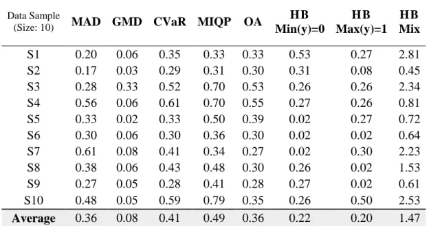
Table 4.1: Comparison of objective function value for data samples of size 10 ... 42
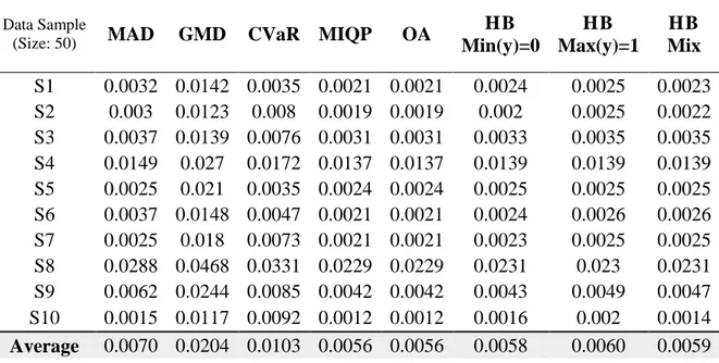
Table 4.2: Comparison of objective function value for data samples of size 50 ……… 42
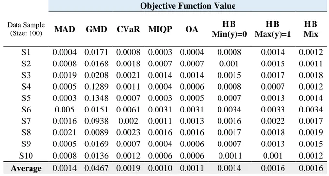
Table 4.3: Comparison of objective function value for data samples of size 100 ……….. 43
Table 4.4: Comparison of objective function value for data samples of size 1000 ……… 44
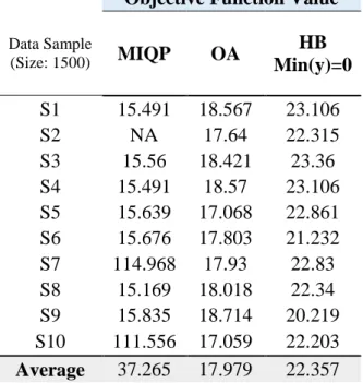
Table 4.5: Comparison of objective function value for data samples of size 1500 ……… 44
Table 4.6: Comparison of objective function value for data samples of size 2000 ……… 45
Table 4.7: Comparison of computational time for data samples of size 10 ……… 45
Table 4.8: Comparison of computational time for data samples of size 50 ……… 46
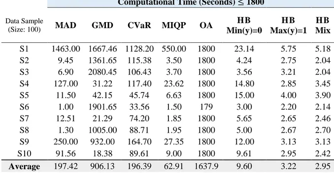
Table 4.9: Comparison of computational time for data samples of size 100 ……….. 46
Table 4.10: OA results in 60 seconds for data samples of size 100 ……… 47
Table 4.11: Objective value based on matrix 𝛴 = 𝐼 ……….... 48
Table 4.12: Objective Values based on small k ……….. 50
Table 4.13: Computational time based on small k ……….. 50
LIST OF FIGURES
Figure 1.1: Systematic and Unsystematic risk ……….... 5
Figure 1.2: Portfolio efficient frontier curve ………... 6
Figure 1.3: Capital Market Line ……….. 7
Figure 1.4: Characteristic Line ... 9
Figure 2.1: The Outer Approximation algorithm ………... 29
LIST OF SYMBOLS AND ABBREVIATIONS
BB Branch-and-Bound
CAPM Capital Asset Pricing Model CML Capital Market Line
CVaR Conditional Value at Risk GMD Gini Mean Difference HB Heuristic Branching MAD Mean Absolute Deviation
MINLP Mixed Integer Nonlinear Programming MIQP Mixed Integer Quadratic Programming MV Mean-Variance
NLP Nonlinear Programming OA Outer Approximation QP Quadratic Programming VaR Value at Risk
CHAPTER 1 INTRODUCTION
1.1. Context
One of the most important concerns of investors of all time is to choose the best investing opportunities to maximize the value of their investment. Making decision on investment options is very important, challenging and complex especially for large financial institutions such as banks, insurance, investing and commercial institutions, real states and public sectors who seeks for high return opportunities at a reasonable risk. There is a variety of investing options that one might consider like stocks, bonds, gold, etc. but none of them is the best choice ever that means a rational person looks for a combination to spread the risk of loss which is known as diversification. A diversified portfolio has a smoother risk behavior that is less variation in expected return. Risk arise from uncertainty of data like future investment return which is forecasted. Well-diversification helps to decrease volatility of portfolio performance since, assuming that a portfolio assets are normally distributed, then the price of all assets does not change in the same direction at the same time and at the same rate otherwise the portfolio won’t be well-diversified (Mansini et al., 2015; Moyer et al., 2006).
There are two sides for an investment namely Risk and Return. As a general rule in economy, one who seeks more return must expect more risk too and vice versa. An investor can be classified in one of the three categories; risk-averse is someone who avoid from taking risk thus so conservative, risk-taker on the contrary is ready to take more risk hoping to gain more return and risk-indifferent who is neither risk-averse nor risk-taker. As a matter of fact, although risk-takers are receptive for more risk but they all, as a rational person, requires a certain level as the minimum accepted return on investment for safety (Brigham & Houston, 2007).
The objective of financial decision makers is to maximize the value of investment projects for its owners that is to maximize shareholders’ wealth which is measured by the market price of investing options say common stock. Market value (price) is defined as the price at which the stock trades in
the marketplace. In other words, the higher return does not mean more value on investment due to associated risk. Risk and return are part and parcel of investment that has to be considered simultaneously (Brigham & Ehrhardt, 2008).
1.2. Organization of the thesis
This thesis composed of the following chapters to cover the relevant literature and proposed methodological approach to deal with the topic of this thesis. Here is a brief of what has been discussed in each chapter.
Chapter (1) begins with the introduction to the context of the problem and its affiliated attributes following by the contribution of the thesis. The rest of the chapter is devoted to a concise definition of the financial market, its types and effects to the problem at hand. At the end, the concept of risk and return and their correlation will be explained as well as the concept of diversification.
Chapter (2) will collect and compile the relevant literature in field of portfolio management containing portfolio optimization problem, portfolio optimization with real features in the market which mainly focuses on the two complicating features so called Cardinality constraint and bounds on investment that are the case of our problem. In the following, the most important methods to deal with the problem will be introduced addressing their pros and cons. A class of optimization problems named MINLPs and different approaches to solve them are discussed comprising some applicable and efficient bounding method for MINLP to generate a lower and upper bound to limit the domain of optimal value. Finally, some techniques such as adding valid inequalities and branching rules for tightening the gap between lower and upper bound thus improving the solution precision are investigated.
Chapter (3) will discuss about required methods and algorithmic approaches to deal with our problem. These methods include Outer Approximation algorithm and proposed Heuristic Branching algorithm compared with Branch-and-Bound as an exact global solution using CPLEX.
Chapter (4) is devoted to compare the numerical results of the proposed heuristic branching algorithm and outer approximation method versus most applicable methods from literature in terms of optimal value and time budget. All the results are obtained by executing random data that empirically tested.
1.3. Contribution
This research is focused on the Markowitz Mean-Variance (MV) portfolio optimization problem with cardinality constraints and bounding on variables so called as modern portfolio optimization problem which is a MINLP problem and well known as an NP-Hard problem. The problematic is that exact methods like branch and bound/cut solved even by CPLEX are not able to solve large instances in a reasonable time due to complexity of covariance matrix structure. In other words, as more securities included in portfolio, it increases the calculations geometrically since for the covariance matrix the number of correlation coefficient to be considered is 𝑛(𝑛 − 1)/2 independent entries thus a large number of combination has to be computed to choose the best uncorrelated assets from the covariance matrix. Such complexities and the need for choosing optimal portfolio in a reasonable time in real stock market in which the transactions have to be fast, requires an efficient method to solve the portfolio selection problem considering a trade-off between solution quality and computational time which is the aim of this research.
The contribution of this research is twofold: First, a heuristic branching algorithm is proposed such that by finding a lower and upper bound and applying branching rules based on a cut, it produces near-optimal solution with acceptable precision and in a very timely manner which is suitable for large instances. Second, an Outer Approximation algorithm has been applied for the first time which shows very competitive results with exact methods. Finally, the results are compared with the other methods in literature and the best methods in different scales are classified. All the results have been empirically tested.
1.4. Financial Market
A financial market is a market in which people trade financial securities, commodities, and other fungible items of value at low transaction costs and at prices that reflect supply and demand. Securities include stocks and bonds, and commodities include precious metals or agricultural products. In economics, typically, the term market means the aggregate of possible buyers and sellers of a certain goods or service and the transactions between them. A securities market is used in an economy to attract new capital, transfer real assets in financial assets, determine price which will balance demand and supply and provide a means to invest money both short and long term (Brigham & Houston, 2007; Brigham & Ehrhardt, 2008).
1.5. Risk and Return
The risk is defined as the possibility that actual future returns will deviate from expected returns. In other words, it represents the variability of returns. From the perspective of security and investment analysis, risk is the possibility that actual cash flows (returns) will be different from
forecasted cash flows (returns). An investment is said to be risk-free if the money returns from the
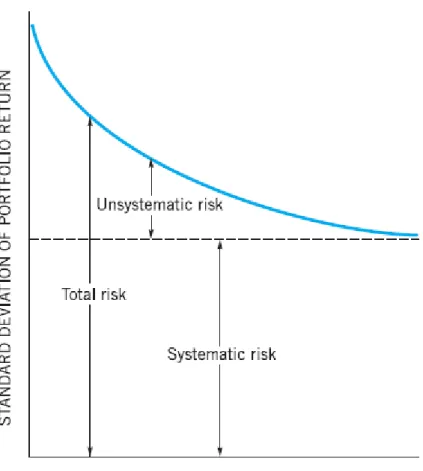
initial investment are known with certainty. Some of the best examples of risk-free investments are U.S. Treasury securities. There are two categories of risks; systematic and unsystematic. Systematic (Market) risk arise from overall economic and industry condition and is inherent in the nature of the business thus it is beyond management control and con not be reduced. Unsystematic risk, from the other side, is a result of miss-management, low forecasting accuracy or any other shortcoming in the process of planning or decision making which can be reduced by more logical and correct decisions. Consequently, unsystematic risk is under control, although it con not be totally eliminated but it could be substantially decreased (see figure 1.1) (Moyer et al., 2006).
1.6. Portfolio diversification
Diversification is a way to lessen unsystematic risk in portfolio. The idea behind diversification is to spread investment budget over a set of assets to create a portfolio of diverse assets hence spreading the risk. The logic of holding diverse assets is that the price of diverse assets does not
change in the same direction and at the same time or at the same rate. Technically, combining assets with negatively correlated returns and lower correlations, significantly reduces the total variability or dispersion (i.e. risk) of portfolio return. In other words, “do not put all your eggs in one basket”.
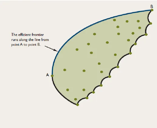
A portfolio called efficient if for a given expected return, no other portfolio has a lower risk and vice versa that is for a certain level of risk, no other portfolio has higher expected return. The curve which connect the efficient portfolios A and B as shown in figure 1.2 is called efficient frontier. Selecting optimal portfolio whether to maximize return or minimize risk, depends on the investor’s degree of risk reception. More conservative (risk averse) investors choose their optimal portfolios among efficient portfolios (Moyer et al., 2006).
Evaluating portfolio risk performance when there are more securities included increases the calculations geometrically since for the covariance matrix the number of correlation coefficient to be considered is n (n - 1) /2 independent entries thus a large number of sample has to be computed to choose the best uncorrelated assets from the covariance matrix. (Tapiero, 2004; Mansini et al., 2015).
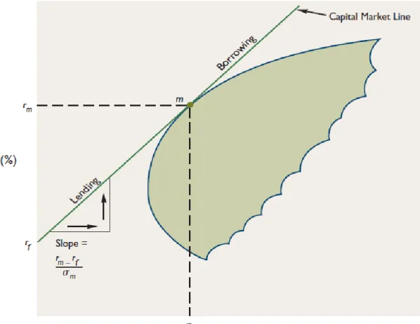
Let 𝑟𝑓 denote the risk-free rate of return and m the market portfolio with market rate of return 𝑟𝑚 and standard deviation 𝜎𝑚 as market risk in state of market equilibrium. The line connecting 𝑟𝑓 and
m as shown in figure 1.3 is called capital market line (CML). The slope of the capital market line
measures the portfolio market price at equilibrium. If investors are able to lend and borrow money at the rate 𝑟𝑓, then any risk-return combination on the capital market line can be achived by
investing (i.e. lending) a pert of money on risk-free assets and the rest in portfolio m (between 𝑟𝑓
and m on the CML) or by borrowing money at the rate 𝑟𝑓 and investing them in portfolio m (above
m on the CML). Risk-averse investors tend to minimize risk and invest at around point 𝑟𝑓 and more risk-takers around point m on the capital market line hoping to gain more return (Moyer et al., 2006).
A widespread method to analyze the relationship between risk and return is Capital Asset Pricing Model (CAPM). However, all models are subject to data estimation errors, and possibly to modeling errors.
1.7. Capital Asset Pricing Model (CAPM)
𝐶𝑜𝑠𝑡 𝑜𝑓 𝐸𝑞𝑢𝑖𝑡𝑦 = 𝑅𝑓+ 𝛽(𝑅𝑚− 𝑅𝑓)
Rf is the rate of return on a risk-free investment (i.e. Government bonds or Treasury Bills). Treasury
bill is Short-term security sold by a central bank to meet a government’s short-term financial requirements. Treasury bills are easily sold and have a relatively low rate, but they are nearly risk-free and are exempt from taxes.
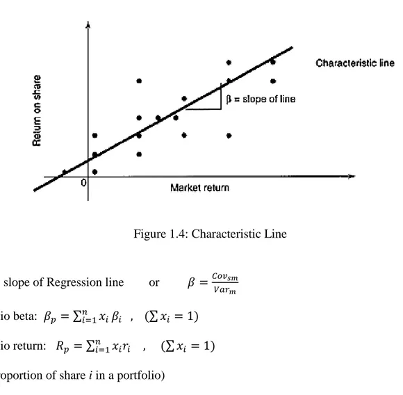
β is a measurement of the relative risk of a specific share to the market as a whole. (A beta share greater than 1 is considered to have greater risk than the market, and a beta share less than 1 is considered to have less risk than the market.)
Rm is the average rate of return on the market as a whole over the period being analyses.
(Rm - Rf) represents the market risk premium, or the difference in rates of return between
investments that are considered risk-free, such as government bonds, and those investments that are market driven, over the period being analyses.
Risk premium [𝛽(𝑅𝑚− 𝑅𝑓)]: Extra return expected from a risky asset compared with the return from an alternative risk-free asset.
Notice: β is Systematic (Market) Risk that cannot be eliminated by portfolio diversification.
β = the slope of Regression line or 𝛽 =𝐶𝑜𝑣𝑠𝑚 𝑉𝑎𝑟𝑚
Portfolio beta: 𝛽𝑝 = ∑𝑛𝑖=1𝑥𝑖𝛽𝑖 , (∑ 𝑥𝑖 = 1)
Portfolio return: 𝑅𝑝 = ∑𝑛𝑖=1𝑥𝑖𝑟𝑖 , (∑ 𝑥𝑖 = 1)
(𝑥𝑖 : proportion of share i in a portfolio)
Therefore, if a particular security's price movement is greater than the prescribed benchmark, a value of β > 1 is given. This constitutes a volatile or risky security, whereas β < 1 is treated as an investment that involves a low amount of risk (Stoyan, 2009).
CHAPTER 2 LITERATURE REVIEW
2.1. Portfolio Optimization Problem
An investor seeks to invest his money in a number of different securities (stock, bonds, etc.) such that having minimum risk for a certain return. There are two main types of risks associated with investment; (1) the risk of having less return as expected for securities, (2) the risk of not well-diversified portfolio, which stems from not having enough different types of securities in portfolio. Consider an investor who has a certain amount of money to be invested in a number of different securities (stocks, bonds, etc.) with random returns. Let 𝜇𝑖 be expected return and 𝜎𝑖2 covariance for each security 𝑖 = 1, ⋯ , 𝑛. In addition, for any two securities i and j, their correlation coefficient 𝜌𝑖𝑗 is also assumed to be known. Let 𝑥𝑖 represent the proportion of the total funds invested in
security i, then the expected return and the variance of the portfolio 𝑥 = (𝑥1, ⋯ , 𝑥𝑛) are as follows 𝐸[𝑥] = 𝑥1𝜇1 + ⋯ + 𝑥𝑛𝜇𝑛 = 𝜇𝑇𝑥
𝑉𝑎𝑟[𝑥] = ∑ 𝜌𝑖𝑗 𝑖,𝑗
𝜎𝑖𝜎𝑗𝑥𝑖𝑥𝑗 = 𝑥𝑇Σ 𝑥
Where 𝜌𝑖𝑖 ≡ 1, Σ𝑖𝑗 = 𝜌𝑖𝑗𝜎𝑖𝜎𝑗 and 𝜇 = (𝜇1, ⋯ , 𝜇𝑛).
A feasible portfolio 𝑥 is called efficient if with a certain amount of risk, it provides the maximum expected return or, vice versa, having a certain expected return among all securities, it has minimum risk value. The collection of efficient portfolios forms the efficient frontier of the portfolio universe (Cornuejols & Tutuncu, 2006; Prigent, 2007).
The standard portfolio optimization problem model known as the Markowitz’ Mean-Variance portfolio optimization model can be formulated in three equivalent ways as bellow;
(1) The first model aims to minimize the portfolio variance for securities 1 to n respecting at least a target value R as expected return. In this case, the objective is a convex quadratic function over a set of linear constraints:
min 𝑥 𝑥 𝑇Σ 𝑥 𝜇𝑇𝑥 ≥ 𝑅 𝑒𝑇𝑥 = 1 𝑥 ≥ 0
where e is an n-dimensional sum vector (all of its components are equal to 1). The first constraint requires a target value as the minimum expected return. The second constraint indicates that the investment proportions in different securities 𝑥𝑖 should sum to 1. Non-negativity constraints on 𝑥𝑖
are introduced to prevent short sales (selling a security that you do not have).
(2) The second model tries to maximize the expected return of portfolio considering a tolerance limit for portfolio risk.
max 𝑥 𝜇 𝑇𝑥 𝑥𝑇Σ 𝑥 ≤ 𝜎2 ∑𝑛𝑖=1𝑥𝑖 = 1 𝑥 ≥ 0
(3) The last model combines the expected return and weighted risk as objective function. max 𝑥 𝜇 𝑇𝑥 − 𝜆 𝑥𝑇Σ 𝑥 𝑥 ∈ 𝐶 = {𝑥 ∈ ℝ𝑛 | ∑ 𝑥 𝑖 = 1, 𝑥 ≥ 0} 𝑛 𝑖=1
Where λ is the investors risk aversion coefficients vector. Since variance is always non-negative, then
𝑥𝑇Σ 𝑥 ≥ 0 ∀ 𝑥
which means Σ is positive semi-definite.
The all three models proposed above have a worst-case orientation. That is, we try to optimize the behavior of the solutions under the most adverse conditions (Cornuejols & Tutuncu, 2006).
2.2. Portfolio Optimization with Real Feature
In practice, investors have different preferences or limitations to be considered in portfolio selection which stem from real features in the market that might not be taken into account in the model such as restricting the number of assets selected (cardinality constraint), bounding on the amount of money invested in an asset (bound constraints), transaction costs and decision dependency requirements (logical constraints) (Mansini et al., 2015; Maringer, 2005).
2.2.1. Cardinality Constraints
According to modern portfolio theory, the investors aimed to minimize risk with a certain level of return. A well-diversified portfolio reduces unsystematic risk which is influenced by decision so it is under control through logical decision making. Investing in many assets with small amount will increase the total risk as well as total cost due to fixed transaction costs associated to the number of assets in portfolio incurred when buying or selling assets. On the other side, investing on a few assets increases the opportunity loss cost of not choosing the best combination out of all assets also not well spreading risk over assets thus not a well-diversified portfolio. As a result, investors prefer to restrict the number of assets to be held in portfolio. A restriction on the number of assets that can be selected in a portfolio is called cardinality constraint (Mansini et al., 2015).
In order to impose the cardinality constraint in a portfolio optimization model first we define binary variables 𝑦𝑖 ∶ 𝑖 = 1, . . . , 𝑛, where 𝑦𝑖 is equal to 1 if asset i is selected in the portfolio, and 0
otherwise. The cardinality constraint can be expressed by restricting the number of assets in portfolio not to be greater than a predefined number Kmax and not lower than a minimum number Kmin:
𝐾𝑚𝑖𝑛≤ ∑ 𝑦𝑖 𝑛
𝑖=1
≤ 𝐾𝑚𝑎𝑥
2.2.2. Bounds on Investment
A very practical limitation in financial decision making is to enforce decision variables to take values within a given interval by applying lower and upper bound limit on the share 𝑥𝑖 or on the
amount of an asset held in the portfolio. These constraints are also known as threshold constraints. Such a constraint is formulated as:
𝑙𝑖 ≤ 𝑥𝑖 ≤ 𝑢𝑖 ∀ 𝑖 = 1, . . . , 𝑛
If the bounds on investment is applicable only if the asset is selected in the portfolio, the above constraint will be modified using the binary variables 𝑦𝑖 as follow (Mansini et al., 2015).
𝑙𝑖𝑦𝑖 ≤ 𝑥𝑖 ≤ 𝑢𝑖𝑦𝑖 ∀ 𝑖 = 1, . . . , 𝑛
2.3. Problematic
The classical Mean-Variance (MV) portfolio selection model is the pillars of modern portfolio theory. However, there has been several criticism to model addressing the nonrealistic assumptions such as normal behavior of portfolio risk and non-well-diversified securities in portfolio.
One of the most important refinements that have been proposed to make the model more realistic is to limit the number of assets to be held in an efficient portfolio so-called cardinality constraint. The other refinement recommends lower and upper bounds on the proportion of the investment in each asset named as quantity constraints. The last requirement comes from the truth that a very small investment in some securities is not beneficial because of transactions costs. The Markowitz model with the above requirements is called Limited Asset Markowitz Model (LAM).
According to Cesarone et al (2010), in order to define the LAM model, the realistic constraint that at maximum K assets should be held in the portfolio (called cardinality constraint) and the quantity of 𝑥𝑖 for each asset that is included in the portfolio should be limited within a given interval [𝑙𝑖 , 𝑢𝑖]
(a quantity constraint or buy-in threshold), will be added to Markowitz classical model as Model 2.1:
Model 2.1 Min 𝑥 𝑥 𝑇Σ 𝑥 S.t. 𝜇𝑇𝑥 ≥ 𝑅 ∑ 𝑥𝑖 𝑛 𝑖=1 = 1 𝑥𝑖 = 0 𝑜𝑟 𝑙𝑖 ≤ 𝑥𝑖 ≤ 𝑢𝑖 , 𝑖 = 1, … , 𝑛 |𝑠𝑢𝑝𝑝(𝑥)| ≤ 𝑘 Where 𝑠𝑢𝑝𝑝(𝑥) = {𝑖: 𝑥𝑖 > 0}.
The Model 2.1 has a convex quadratic objective function but the set of constraints is not convex anymore. This problem can be reformulated as a Mixed Integer Quadratic Program (MIQP) with the addition of n binary variables as Model 2.2:
Model 2.2 Min 𝑥 𝑥 𝑇Σ 𝑥 S.t. ∑ 𝜇𝑖 𝑛 𝑖=1 𝑥𝑖 ≥ 𝑅 ∑ 𝑥𝑖 𝑛 𝑖=1 = 1 ∑ 𝑦𝑖 𝑛 𝑖=1 ≤ 𝑘 𝑙𝑖𝑦𝑖 ≤ 𝑥𝑖 ≤ 𝑢𝑖𝑦𝑖 , 𝑖 = 1, … , 𝑛 𝑥𝑖 ≥ 0 𝑖 = 1, … , 𝑛 𝑦𝑖 ∈ {0,1} 𝑖 = 1, … , 𝑛
Such an MIQP model is classified as an NP-Hard problem (Cesarone et al, 2010).
According to Cesarone et al (2010), “A number of exact approaches have been proposed to solve the problem above. Bienstock (1996), proposes a branch-and-cut algorithm and reports good computational results for some real-life problems; however, his method seems to become extremely slow for small values of K. Since exact methods are able to solve only a fraction of
practically useful LAM model, a variety of heuristic procedures have also been proposed for solving the problem.”
Different approaches have been proposed to simplify portfolio selection model like approximating the quadratic objective function with linear one. These approaches make use of the approximation or the decomposition of the covariance matrix. Some other studies applied a different linear function, which leads to the same goal. For example, using the mean absolute deviation (MAD) model. One another important risk measurement tool is Value-at-Risk (VaR), but the VaR optimization problem is not convex, also it does not benefit from diversification. However, Conditional Value at Risk (CVaR) has been introduced which resolves difficulties of VaR but still it is an approximation to the original function.
The following will shortly review the LP optimization model which outperforms among the others and will be compared with the proposed heuristic method in this research.
Mean Absolute Deviation (MAD) Gini Mean Difference (GMD) Conditional Value at Risk (CVaR)
2.4. Mean Absolute Deviation (MAD)
An alternative to the standard deviation (SD) as common error measurement is the Mean Absolute Deviation (MAD), which provide a linear function however, its value is always less than SD since it does not consider the correlation among variables.
𝑀𝐴𝐷 = 𝐸 |∑ 𝜇𝑗𝑥𝑗 − 𝐸 (∑ 𝜇𝑗𝑥𝑗 𝑛 𝑗=1 ) 𝑛 𝑗=1 |
For normally distributed variables the following ratio holds 𝑀𝐴𝐷 𝑆𝐷 = 𝐸|𝑋| √𝐸(𝑋2) = √ 2 𝜋= 0.79788
It has been shown that if the returns are multivariate normally distributed, the minimization of the MAD provides similar results as the classical Markowitz formulation. However, they did not consider cardinality as a discrete model formulation. Also, the assumption “multivariate normally
distributed” returns does not always hold since, in order to reduce unsystematic risk, a portfolio
has to be well diversified which means it should include some complementary and diverse securities. Thus, there exist interrelation among securities and some securities might dominate some others. Such conditions and more does not guarantee the “multivariate normally distributed” assumption (Konno &Yamazaki, 1991) see also (Rudolf et al., 1999).
2.5. Gini Mean Difference (GMD)
Another dispersion metric as a risk measurement for random variables which are independently and identically distributed with the same (unknown) distribution is the Gini’s Mean Difference between each pair of variables.
𝐺𝑀𝐷 = 𝐸|𝑥𝑖 − 𝑥𝑗| = 1 𝑛∑ ∑|𝑥𝑖 − 𝑥𝑗| 𝑛 𝑗=1 𝑛 𝑖=1 ∶ 𝑖 ≠ 𝑗
Similar to MAD, if the rates of return are multivariate normally distributed, minimizing GMD is equivalent to minimizing standard deviation (Mansini, 2015).
2.6. Value at Risk (VaR)
One well-known risk measure is Value at Risk (VaR) which represents the predicted maximum loss with a specified probability level (e.g., 95%) over a given period of time. Given a confidence level 𝛼 ∈ (0,1), the VaR of the portfolio at the confidence level 𝛼 is given by the smallest number γ such that the probability that the loss X exceeds 𝛾 is at most (1 − 𝛼). Mathematically, if X is the loss of a portfolio over a fixed period of time, then 𝑉𝑎𝑅𝛼(𝑋) is the level αquantile, i.e.
Where Ψ(𝑥, 𝛾), is the cumulative distribution function. VaR has one important drawback that is, it lacks subadditivity property. In other words, risk measures should consider risk diversification and therefore, satisfy the following subadditivity property:
𝑓(𝑥1+ 𝑥2) ≤ 𝑓(𝑥1) + 𝑓(𝑥2)
But, 𝑉𝑎𝑅 of two different investment portfolios might be greater than the sum of the individual 𝑉𝑎𝑅s. Also, 𝑉𝑎𝑅 is nonconvex and non-smooth and has multiple local minimum, which makes the problem difficult seeking the global minimum. Another criticism of VaR is that it pays no attention to the magnitude of losses beyond the VaR value. Due to above mentioned shortfalls of VaR a modified alternative named Conditional Value at Risk (CVaR) has been introduced.
CVaR also called "expected shortfall" at 𝛼% level is the expected loss given that the loss exceeds VaR and is an alternative to VaR that is more sensitive to the shape of the loss distribution in the tail of the distribution.
We denote the portfolio choice vector by 𝑥 and the random events by the vector v that has a probability density function denoted by 𝑝(v). Let 𝑓(𝑥, 𝑣) denote the loss function. Then the 𝛼 − 𝐶𝑉𝑎𝑅 for portfolio 𝑥 is defined as:
𝐶𝑉𝑎𝑅𝛼(𝑥) =1 − 𝛼1 ∫ 𝑓(𝑥, 𝑣)𝑝(𝑣)𝑑(𝑣)
𝑓(𝑥,𝑣)≥𝑉𝑎𝑅𝛼(𝑥)
N.B. CVaR of a portfolio is always at least as big as its VaR that is 𝐶𝑉𝑎𝑅𝛼(𝑥) ≥ 𝑉𝑎𝑅𝛼(𝑥).
For discrete probability distribution (where event 𝑣𝑗 occurs with probability 𝑃𝑗 for 𝑗 = 1, ⋯ , 𝑛) the
CVaR becomes (Cornuejols & Tutuncu, 2006).
𝐶𝑉𝑎𝑅𝛼(𝑥) =
1
1 − 𝛼 ∑ 𝑝𝑗𝑓(𝑥, 𝑣𝑗)
𝑗:𝑓(𝑥,𝑣𝑗)≥𝑉𝑎𝑅𝛼(𝑥)
2.6.1. Minimizing CVaR
In order to simplify the function above for optimization, the following function will be considered instead
𝐹𝛼(𝑥, 𝛾) ∶= 𝛾 + 1 1 − 𝛼∫𝑓(𝑥,𝑣)≥𝛾(𝑓(𝑥, 𝑣) − 𝛾)𝑝(𝑣)𝑑(𝑣) Or equivalently 𝐹𝛼(𝑥, 𝛾) ∶= 𝛾 + 1 1 − 𝛼∫(𝑓(𝑥, 𝑣) − 𝛾)+𝑝(𝑣)𝑑(𝑣) The following properties hold for the function above
1. The 𝐹𝛼(𝑥, 𝛾) is a convex function of γ 2. 𝑉𝑎𝑅𝛼(𝑥) is a minimizer over γ of 𝐹𝛼(𝑥, 𝛾)
3. The minimum value over γ of the function 𝐹𝛼(𝑥, 𝛾) is 𝐶𝑉𝑎𝑅𝛼(𝑥)
As a result of these properties, it will be concluded that min
𝑥 𝐶𝑉𝑎𝑅𝛼(𝑥) = min𝑥,𝛾 𝐹𝛼(𝑥, 𝛾)
Since it is not desirable to compute density function P(V) of random events, we assume a number of scenarios (𝑣𝑖: 𝑖 = 1, ⋯ , 𝑆) with same probability. In this case, we obtain the following approximation to the function 𝐹𝛼(𝑥, 𝛾) by using the empirical distribution of the random events
based on the available scenarios:
𝐹̂𝛼(𝑥, 𝛾) ≔ 𝛾 +
1
(1 − 𝛼)𝑆∑(𝑓(𝑥, 𝑣𝑖) − 𝛾)+
𝑆
𝑖=1
To solve the CVaR portfolio optimization problem using this function, artificial variables 𝑧𝑖 are introduced such that
Min 𝑥,𝑧,𝛾 𝛾 + 1 (1−𝛼)𝑆∑𝑆𝑖=1𝑧𝑖 S.t. 𝑧𝑖 ≥ (𝑓(𝑥, 𝑣𝑖) − 𝛾) ∀ 𝑖 = 1, ⋯ , 𝑆 𝑧𝑖 ≥ 0 ∀ 𝑖 = 1, ⋯ , 𝑆 𝑥 ∈ 𝑋
2.7. Mixed Integer Nonlinear Programming Models
An optimization problem which has nonlinear functions and contains continuous and discrete variables together is known as Mixed Integer Nonlinear Program (MINLP). A general MINLP model could be defined as Model (2.3);
𝑀𝑖𝑛 𝑓(𝑥, 𝑦) 𝑠. 𝑡. 𝑔(𝑥, 𝑦) ≤ 0
ℎ(𝑥, 𝑦) = 0 Model (2.3) 𝑥 ∈ [ 𝑥 , 𝑥 ]
𝑦 ∈ [ 𝑦 , 𝑦 ] 𝑖𝑛𝑡𝑒𝑔𝑒𝑟
Where the vectors 𝑥 ∈ ℝ𝑛 and 𝑦 ∈ ℤ𝑚 are finite and f, g and h: ℝ𝑛 → ℝ are nonlinear functions. In case that f and g are convex and h is affine, the MINLP is convex otherwise, it is nonconvex. This types of problems have vast applications in different fields like economy, finance, engineering, etc. (Nowak, 2005).
A restricted version of MINLP in which only the objective function is nonlinear and the constraints are all linear could be expressed by Model (2.4);
𝑀𝑖𝑛 𝑓(𝑥, 𝑦) 𝑠. 𝑡. 𝐺(𝑥, 𝑦) ≤ 𝑏
𝐻(𝑥, 𝑦) = 𝑑 Model (2.4) 𝑥 ∈ [ 𝑥 , 𝑥 ]
𝑦 ∈ [ 𝑦 , 𝑦 ] 𝑖𝑛𝑡𝑒𝑔𝑒𝑟
Where G and H are rational matrix and b and d are rational vectors. Although, Model (2.4) have simpler linear constraints but still is an MINLP. Both Models (2.3) and (2.4) are classified as NP-Hard problem due to combining nonlinearity and integrality in the model (Junger et al., 2010; Lee & Leyffer, 2012).
2.8. Fundamental methods to solve MINLP
Generally, MINLPs are challenging combinatorial optimization problems which combines integrality and nonlinearity in the problem that each of which arise complexity for the problem. If one removes the integrality from the problem but preserves the nonlinear functions, then MINLP reduces to General Nonlinear program (NLP) which could be NP-Hard. From the other side, restricting the model to contain only linear functions but maintaining integer variables, the MINLP reduces to Mixed-Integer Linear program (MILP) that are easier to solve but could be difficult especially for very large instances. However, under certain conditions NLP will be easier to solve efficiently. If in MINLP, the objective function and all constraints are convex and bounded, thanks to properties of convexity, relaxing integrality leads to a convex NLP problem for which there exist efficient algorithms (Lee & Leyffer, 2012).
From algorithmic and solvers perspective, there is a giant gap between MINLP and MIP. With state-of-the-art solvers, an MIP could be solved for large scale problems even with millions of variables and constraints (not in the worst case) while the dimension of solvable MINLPs is often limited by a number that is smaller by three or four orders of magnitude. One may consider a linear approximation of nonlinear functions to transform MINLP to MILP (like piecewise linearization which would be explain further in section 2.8.1) but these approximations are usually poor with low precision and in some cases, it ends up to a very large MILP which could be NP-Hard problem (Nowak, 2005).
There are variety classes of methods to deal with MINLP. However, most of methods apply some form of tree-search. Here is a brief introduction to these class of methods. The first class is so-called Decomposition Methods used to solve large scale problems with separable structure. In this class, if the problem has a block-separable structure, it can be split into several smaller sub-problems each of which corresponds to a separate block of the original MINLP. Sub-sub-problems often hold specific complicated constraints and/or variables and their solutions will be combined through joining (common) constraints in a Master problem which is usually a simple problem containing general constraints. Decomposition methods differ based on their underlying principles
and problem formulation. Such methods are mainly: Dantzig-Wolfe Decomposition, Column Generation, Benders Decomposition, Dual methods – Lagrangian Decomposition and Primal cutting-plane methods (Nowak, 2005).
The second class is based on generating and tightening bounds on the optimal solution of the MINLP. In this class, algorithms solve a sequence of updated sub-problems to generate and improve bounds iteratively until certain stopping criterions has been reached. Here, two fundamental concepts are: Relaxation and Constraint Enforcement. Considering a Minimization problem, Relaxation is used to obtain a lower bound for the problem by dropping integrality from variables or eliminating some constraints resulting in larger feasible set. If all the remaining constraints after relaxation are convex then the feasible set is convex which makes it easier to solve. An upper bound on the optimal solution could be attain from any feasible or heuristic solution. Since, basically heuristic solutions are sub-optimal (does not guarantee global optimality) it can be considered as an upper bound for minimization problem. Now one can apply efficient decisions to tighten either lower or upper bound to approach each other until reaching a given tolerance as termination rule. Constraint enforcement is aimed at excluding the part of feasible solution from the feasible set after relaxation. The feasible solution to be excluded are feasible for the relaxed problem but not for the original MINLP. Constraint enforcement basically carried out by adding
Valid inequalities like valid cuts to update and tightening bounds or by branching scheme which
divides relaxation problem into two or more sub-problems (Belotti et al., 2012).
The third class is so-called meta-heuristic. Some complicated real world problems especially NP-Hard problems cannot be solved to global optimality with the state-of-the-art methods due to complexity or large sizes as well as expensive computational time. However, we are interested to obtain a good solution in a timely manner. In such cases, heuristic methods which does not guarantee optimality but accelerates computations are used. Heuristics differ in search techniques and most of them take advantage of probabilistic search schemes that require a random choice of a candidate solution at each iteration to escape from local optimality trap. Genetic Algorithm (GA), Simulated Annealing (SA), Tabu Search (TS), Ant Colony Optimization (ACO), Particle-Swarm Optimization (PSO), etc. are fall under this category (Belotti et al., 2012).
2.8.1. Piecewise Linearization
A very first idea to deal with nonlinear functions is to make use of a series of piecewise linear function to approximate a nonlinear function. To do so, an interval [a, b] for the nonlinear function
f(x) will be subdivided into smaller intervals with a linear function for each adjacent pairs of points.
Obviously, the more piecewise linear functions, the better and more precise approximation of a nonlinear function. In high dimension the same principle applies like in n-dimension, lines are simplices. Here the difficulty reveals that is the number of simplices needed increases drastically as dimension increases. Thus, using piecewise linearization seems applicable for MINLPs merely if the nonlinear functions have only a few variables and/or smoother function (Lee & Leyffer, 2012).
In this paper the focus is on the second-class methods to cope with MINLP. The following are some relevant and more applicable techniques to find a lower and upper bound for the MINLP and some valid cuts for tightening the bounds on the problem.
2.8.2. Lower Bounds
In this session, some techniques to generate a lower bound, in a relatively cheap way, for general MINLP are discussed. Such a lower bound is essential for branch and bound (BB) type algorithms and are mainly computed through relaxation or underestimations.
Definition 2.1. given an optimization problem
min
𝑥∈𝑆 𝑓(𝑥)
A relaxation for f(x) is any optimization problem of the form min
𝑥∈𝑆̆ 𝑓̌(𝑥)
Such that
𝑆 ⊆ 𝑆̌;
where 𝑓̌(𝑥) is a lower bound for f(x). If 𝑆̌ is a convex set and 𝑓̌ is convex on 𝑆̌, then we have a convex relaxation which can be solved efficiently to optimality (Locatelli & Schoen, 2013).
Integer Variable Relaxation
One way to relax the MINLP is to drop the integrality that is variable 𝑦 ∈ ℤ will be relaxed to 𝑦 ∈ ℝ which reduces MINLP to NLP. Since, relaxation enlarges the feasible set the optimal solution obtained is a lower bound for the original problem.
Constraint Relaxation
Eliminating the constraints containing integer variables from the original model will result in feasible set enlargement and consequently the solution obtained is a lower bound for the original problem but such a relaxation often provides a loose lower bound.
LP-bound
If the integrality is dropped and all nonlinear functions underestimated linearly using any linear approximation (say Taylor linear approximation) then MINLP reduces to LP model that its solution is a lower bound for the MINLP. However, the quality of LP-bound depends on the preciseness of the linear underestimation of nonlinear functions. This type of relaxation for MINLP especially for nonconvex functions usually produces weak bounds (Nowak, 2005).
α-underestimator
Having a continuously twice-differentiable quadratic function 𝑓(𝑥) = 𝑥𝑇𝑄𝑥 + 𝐶𝑇𝑥 over 𝑥 ∈ [ 𝑥 , 𝑥 ], a lower bound such that 𝑓̌(𝑥) ≤ 𝑓(𝑥) could be attained by
𝑓̌(𝑥) = 𝑓(𝑥) − 𝛼 ∑( 𝑥𝑖 𝑛
𝑖=1
Where 𝛼 ≥ 0. For a closer lower bound it is sufficient to set 𝛼 = 𝜆𝑚𝑖𝑛(𝑄) means the minimum eigenvalue of Q, to obtain a convex relaxation. This method can be extended to non-quadratic functions while preserving the validity of the lower bound (Belotti et al., 2012; Nowak, 2005).
2.8.3. Upper Bounds
A class of heuristic methods usually applied to obtain a feasible point as an upper bound for MINLP problem in a timely manner. Some of these heuristics may completely ignore the objective function and focus on finding only a feasible solution.
MILP-based rounding
Finding a locally optimal solution to the continuous relaxation of the MINLP is usually easier and computationally faster than solving the MINLP itself. Given a solution 𝑥̂ of the continuous relaxation, one can try rounding fractional values of integer-constrained variables to obtain a feasible solution around 𝑥̂ as an upper bound. However, such a rounding may end up with an infeasible solution (Belotti et al., 2012).
Feasibility pump
The main idea, like that in MILP based rounding described above, is that an NLP solver can be used to find a solution that satisfies nonlinear constraints. Integrality is enforced by solving an MILP. An alternating sequence of NLP and MILP is solved that may lead to a solution feasible to the MINLP. The main difference from the rounding approach is the way MILP is set up (Belotti et al., 2012).
Undercover
The Undercover heuristic is specially designed for nonconvex MINLPs. The basic idea is to fix certain variables in the problem to specific values so that the resulting restriction becomes easier to solve (Belotti et al., 2012).
2.8.4. Valid cuts
Valid cuts are like redundant constraints that do not cut off any part of feasible region of the original problem which contain potential solution points. In fact, valid cuts used to cut out a portion of relaxed problem that does not hold solution points in order to tighten the lower / upper bound in a repetitive manner thus improving the solution. Valid cuts are divided into general and specific cuts. General cuts can be used for most of the problems but basically, they are not as efficient as specific cuts which are defined specifically for a given problem. A common idea is to use valid inequalities to derive branching rules or selecting the most violated cut at the optimal solution of the relaxation problem to be added to the model to tighten the optimality gap or making decision on variables.
Definition 2.2.
An inequality 𝜋𝑇𝑥 ≤ 𝜋
0 is a valid inequality for 𝑋 ⊆ ℝ𝑛 if 𝜋𝑇𝑥 ≤ 𝜋0 is satisfied by all 𝑥 ∈ 𝑋.
Mixed-integer Rounding Cuts
This types of cut are added iteratively to remove fractional solutions from relaxation problem. Let’s define the set S:
𝑠 ∶= {(𝑥, 𝑦) ∈ ℝ×ℤ | 𝑦 ≤ 𝑏 + 𝑥 , 𝑥 ≥ 0} Let 𝑓0 = 𝑏 − ⌊𝑏⌋, then the inequality
𝑦 ≤ ⌊𝑏⌋ + 𝑥 1 − 𝑓0
is valid for x by verifying it for two cases: 𝑦 ≤ ⌊𝑏⌋ and 𝑦 ≥ ⌊𝑏⌋ + 1 (Belotti et al., 2012). For more detail see (Wolsey, 1998).
Perspective Cuts for MINLP
In many problems, a binary variable is utilized to model a continuous variable upper bound. If y and x are binary and continuous variable respectively, the relationship is as follow:
𝑥 ≤ 𝑢𝑦
According to Belotti et al., (2012) if the continuous variable shows up in a convex nonlinear constraint, then a reformulation technique known as perspective cut can be used for strengthening relaxation. One can define the set S:
𝑆 = {(𝑥1, 𝑥2, 𝑦) ∈ ℝ2×{0,1} ∶ 𝑥2 ≥ 𝑥12, 𝑢𝑦 ≥ 𝑥1 ≥ 0}
Such that the set S is the union of two convex sets: 𝑆 = 𝑆0∪ 𝑆1, where
𝑆0 = {(0, 𝑥2, 0) ∈ ℝ3 ∶ 𝑥2 ≥ 0} ,
𝑆1 = {(𝑥1, 𝑥2, 1) ∈ ℝ3 ∶ 𝑥2 ≥ 𝑥12, 𝑢 ≥ 𝑥1 ≥ 0} .
Now the convex hull of S can be defined as
𝑐𝑜𝑛𝑣(𝑆) = {(𝑥1, 𝑥2, 𝑦) ∈ ℝ3 ∶ 𝑥2𝑦 ≥ 𝑥12 , 0 ≤ 𝑥1 ≤ 𝑢𝑦, 0 ≤ 𝑦 ≤ 1, 𝑥2 ≥ 0}
“The term 𝑥2𝑦 ≥ 𝑥12 plays the role of perspective function. For a convex function 𝑓 ∶ ℝ𝑛 → ℝ ,
the perspective function 𝑃 ∶ ℝ𝑛+1 → ℝ of f is
𝑃(𝑥, 𝑧) ≔ {0 𝑖𝑓 𝑧 = 0,𝑧𝑓(𝑥 𝑧⁄ ) 𝑖𝑓 𝑧 > 0.
If z indicates binary variable that push variable 𝑥 = 0 otherwise, the convex nonlinear constraint 𝑓(𝑥) ≤ 0 must hold, then replacing the constraint 𝑓(𝑥) ≤ 0 with 𝑧𝑓(𝑥 𝑧⁄ ) ≤ 0, results in a convex inequality that significantly tightens the relaxation of feasible region.”
Disjunctive Inequality
Consider two sets of constraints that we are interested to satisfy one of them, then an inequality called disjunctive inequality is used for the union of two sets.
If ∑𝑗∈𝑁𝜋𝑗1𝑥𝑗 ≤ 𝜋01 is valid for 𝑆1 ⊂ 𝑅+𝑛 and ∑𝑗∈𝑁𝜋𝑗2𝑥𝑗 ≤ 𝜋02 is valid for 𝑆2 ⊂ 𝑅+𝑛 , then ∑ 𝑚𝑖𝑛
𝑗∈𝑁
(𝜋𝑗1, 𝜋
𝑗2)𝑥𝑗 ≤ 𝑚𝑎𝑥(𝜋01, 𝜋02)
is valid for 𝑆1∪ 𝑆2 (Nemhauser & Wolsey, 1999).
Level Cuts
Level cuts are based on the idea that in each iteration the objective function value shall not exceed its previous iteration value. For 𝑚𝑖𝑛{𝑓(𝑥) | 𝑔(𝑥) ≤ 0}, if 𝑧̅ indicate an upper bound of the optimal value which can be obtained by 𝑓(𝑥̂) at a feasible point 𝑥̂ or by maximizing f(x) over convex relaxation of the feasible set, then the linear level cut bellow
𝑓(𝑥) ≤ 𝑧̅
is a valid cut for the problem. A nonlinear level cut also can be formulated by 𝐿(𝑥, 𝜇̂) ≤ 𝑧̅
Where 𝐿(𝑥, 𝜇̂) = 𝑓(𝑥) + 𝜇̂𝑇𝑔(𝑥), is a convex Lagrangian underestimating-relaxation (Nowak, 2005).
Some other valid cuts
a) Consider an MINLP problem 𝑚𝑖𝑛{𝑓(𝑥) | 𝑔(𝑥) ≤ 0}, 𝑓: ℝ𝑛 ↦ ℝ 𝑔: ℝ𝑛 ↦ ℝ𝑚 and its Lagrangian function
𝐿(𝑥, 𝜇) = 𝑓(𝑥) + 𝜇𝑇𝑔(𝑥)
where 𝜇 ∈ ℝ+𝑚. A lower bound (𝑓) for the problem can be computed by 𝑓 = min𝑥 𝐿(𝑥, 𝜇)
𝑓 ≤ 𝐿(𝑥, 𝜇) ≤ 𝑓̅ + 𝜇𝑇𝑔(𝑥)
then the following valid inequality can be defined (Nowak, 2005). 𝑔𝑖(𝑥) ≥ −𝜇1
𝑖(𝑓 − 𝑓)
b) Multiplication of two constraints also leads to a valid inequality for MINLP. Having 𝑔(𝑥) ≤ 0 and ℎ(𝑥) ≤ 0 then, −𝑔(𝑥) . ℎ(𝑥) ≤ 0 is a valid cut (Nowak, 2005).
2.9. Outer Approximation (OA) Algorithm
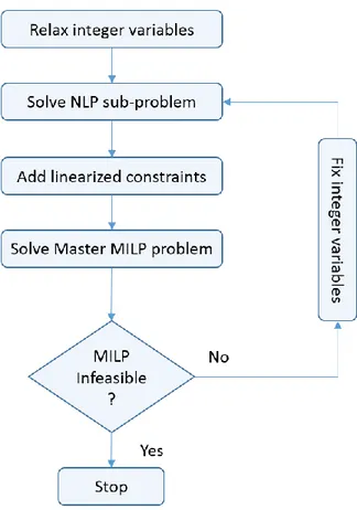
According to Conejo et al. (2006), one standard method to deal with MINLP is outer linear approximation algorithms in which in general, the original MINLP problem is first relaxed then nonlinear functions will be replaced by their linear approximation into the original problem as Master problem. Further, in each iteration the linear approximation of nonlinear functions at the current solution will be added sequentially to either relaxed or master problem as a cut to tighten the bounds on optimal value, until certain stopping criteria reached. Duran and Grossmann (1986) proposed the following outer approximation (OA) algorithm.
1- First relax the integer variables within their bounds and solve the resulting NLP problem. 2- Then a linear approximation of the nonlinear functions at the optimal solution of the
relaxation will replace the nonlinear functions which leaves a MILP problem called Master problem.
3- Solve Master problem.
4- Fix the integer solution of the Master problem in NLP (in step.1) and solve the NLP again. 5- Again, a linearization of nonlinear functions of MINLP at the optimal solution of step.4
will be added to the Master problem.
6- Repeat steps 3 to 5 until the Master MILP problem becomes infeasible or one of the termination criteria (e.g. iteration/time limit) is satisfied.
Linear approximations are constructed by using the gradient of each nonlinear function in the NLP problem at the optimal solution of the NLP problem. The formula for the linearization of a scalar nonlinear inequality 𝑔(𝑥) ≤ 0 at a given point (𝑥0) is as follow.
𝑔(𝑥0) + ∇𝑔(𝑥0)𝑇(𝑥 − 𝑥0) ≤ 0
The flow diagram of the OA algorithm is illustrated in figure 2.1 (Duran and Grossmann, 1986).
Quesada and Grossmann (1992) noticed that for convex problems, the classic outer approximation method spend a lot of time to solve MIP, thus they proposed an outer approximation algorithm (sometimes called the LP/NLP-Based Branch-and-Bound algorithm) in which the need for restarting branch-and-bound tree search is avoided and only a single branch-and-bound tree is
required. For convex problems, the algorithm will terminate if the objective of the MILP problem becomes larger than the objective of the NLP problem (in case of minimization). If the feasible region is convex then its linear approximation does not cut off any portion of solutions. Another general outer linearization algorithm is explained in Conejo et al. (2006).
Quesada and Grossmann (1992) outer approximation algorithm is as follow.
1. First relax the integer variables within their bounds and solve the resulting NLP problem. 2. Linearize nonlinear constraints at optimal solution of the relaxation and replace nonlinear
constraints with the resulting linear constraints to create Master MILP problem. 3. Solve the master MILP problem using a branch-and-bound solver.
4. Whenever the branch-and-bound solver finds a new incumbent solution do:
4.1. Solve the NLP problem by fixing the integer variables to the values in the incumbent solution.
4.2. Add linearization around the optimal NLP solution as lazy constraints to the master MILP problem.
4.3. Continue branch-and-bound enumeration.
5. Terminate MILP solver if the optimality gap is sufficiently small.
CHAPTER 3 METHODOLOGY AND MODELS
This chapter will review the problem to be solved and covers the methods that have been used to cope with the problem in comparison with Branch-and-Bound as an exact global solution. These methods include Outer Approximation algorithm as a general algorithm for MINLP as well as detailed description of the proposed Heuristic Branching algorithm.
Notations: Sets:
𝑖 ∈ 𝐼 : set of assets, 𝐼 = {𝑖 , 𝑖 = 1, ⋯ , 𝑁} where N is the total number of assets.
Variables:
𝑥𝑖 : proportion of funds to be invested in asset i
𝑦𝑖 : binary decision variable equal to 1 if asset i selected and 0, otherwise
Parameters:
𝜇𝑖 : rate of return for asset i Σ : covariance matrix
𝑅 : investor’s minimum expected rate of return for portfolio 𝐾 : maximum number of assets to be hold in portfolio 𝑙𝑖 : lower bound on variable 𝑥𝑖 if it’s selected
𝑢𝑖 : upper bound on variable 𝑥𝑖 if it’s selected
A feasible portfolio 𝑥 is called efficient if with a certain amount of risk, it provides the maximum expected return or having a certain expected return (R), it has minimum risk value. Recall the problematic from section 2.3 so called LAM as in Model 3.1
Model 3.1 Min 𝑥 𝑥 𝑇Σ 𝑥 S.t. ∑ 𝜇𝑖 𝑛 𝑖=1 𝑥𝑖 ≥ 𝑅 ∑ 𝑥𝑖 𝑛 𝑖=1 = 1 ∑ 𝑦𝑖 𝑛 𝑖=1 ≤ 𝑘 𝑙𝑖𝑦𝑖 ≤ 𝑥𝑖 ≤ 𝑢𝑖𝑦𝑖 , 𝑖 = 1, … , 𝑛 𝑥𝑖 ≥ 0 𝑖 = 1, … , 𝑛 𝑦𝑖 ∈ {0,1} 𝑖 = 1, … , 𝑛
Since variance is always non-negative, then 𝑥𝑇Σ 𝑥 ≥ 0 for all x which means Σ is positive
semi-definite. Model 3.1 has a convex quadratic function over a set of linear constraints. Such an MIQP model is classified as an NP-Hard problem due to combining nonlinearity and integrality in the model (Cesarone et al, 2010). Model 3.1 could be solved with CPLEX using Branch-and-Bound as a global optimal solution but restricted to small instances. In the following sections the Outer Approximation algorithm and proposed Heuristic Branching algorithm are described to overcome the problem difficulty for large size problems.
3.1. Outer Approximation Algorithm
One standard method to deal with MINLP is outer linear approximation algorithms in which in general, the original MINLP problem is first relaxed then nonlinear functions will be replaced by their linear approximation into the original problem as Master problem. Further, in each iteration the linear approximation of nonlinear functions at the current solution will be added sequentially to either relaxed or master problem as a cut to tighten the bounds on optimal value, until certain stopping criteria reached. The following is the Duran and Grossmann (1986) proposed Outer Approximation (OA) algorithm that we applied for Model 3.1. Let’s say P: iteration counter and
Iteration counter 𝐏 ∶= 𝟎
Relax integer variables within their bounds in Model 3.1 (𝑦𝑖 ∈ [0,1] ∀ 𝑖 ∈ 𝐼) which leaves a NLP called Relaxed problem.
Iteration counter 𝐏 ∶= 𝟏
Solve Relaxed problem which provides a lower bound for Model 3.1. Denote the optimal solution of relaxed problem by 𝑥1.
Iteration counter 𝐏 ∶= 𝟐
Replace non-linear functions of Model 3.1 with linear approximation at the optimal solution 𝑥1
which leaves a MIP called Master problem. Solve the Master problem and denote the solution by 𝑥2. Master Problem 𝑀𝑖𝑛 𝑍 s.t. (𝑥1)𝑇Σ 𝑥1+ ∇((𝑥1)𝑇Σ 𝑥1)(𝑥 − 𝑥1) ≤ 𝑍 ∑ 𝜇𝑖 𝑛 𝑖=1 𝑥𝑖 ≥ 𝑅 ∑ 𝑥𝑖 𝑛 𝑖=1 = 1 ∑ 𝑦𝑖 𝑛 𝑖=1 ≤ 𝑘 𝑙𝑖𝑦𝑖 ≤ 𝑥𝑖 ≤ 𝑢𝑖𝑦𝑖 𝑖 = 1, … , 𝑛 𝑥𝑖 ≥ 0 𝑖 = 1, … , 𝑛 𝑦𝑖 ∈ {0,1} 𝑖 = 1, … , 𝑛
Iteration counter 𝐏 ∶= 𝟑
Fix integer solution of the Master problem (𝑥2𝐼) in Relaxed problem and solve it again. Denote the
optimal solution of iteration 𝑃 ∶= 3 by 𝑥3.
Iteration counter 𝐏 ∶= 𝟒
Add linear approximation of non-linear functions of Model 3.1 at optimal solution 𝑥3 to the Master
problem and solve the Master problem again. Denote the solution by 𝑥4.
𝑀𝑖𝑛 𝑍 s.t. (𝑥1)𝑇Σ 𝑥1+ ∇((𝑥1)𝑇Σ 𝑥1)(𝑥 − 𝑥1) ≤ 𝑍 (𝑥3)𝑇Σ 𝑥3+ ∇((𝑥3)𝑇Σ 𝑥3)(𝑥 − 𝑥3) ≤ 𝑍 ∑ 𝜇𝑖 𝑛 𝑖=1 𝑥𝑖 ≥ 𝑅 ∑ 𝑥𝑖 𝑛 𝑖=1 = 1 ∑ 𝑦𝑖 𝑛 𝑖=1 ≤ 𝑘 𝑙𝑖𝑦𝑖 ≤ 𝑥𝑖 ≤ 𝑢𝑖𝑦𝑖 𝑖 = 1, … , 𝑛 𝑥𝑖 ≥ 0 𝑖 = 1, … , 𝑛 𝑦𝑖 ∈ {0,1} 𝑖 = 1, … , 𝑛 Iteration counter 𝐏 ∶= 𝟓 to N
Repeat iteration 3 and 4 until Master problem becomes infeasible or one of the termination criteria (e.g. iteration/time limit or optimality gap) is satisfied.
The Outer Approximation algorithm will first find a lower bound in iteration.1 and an upper bound in iteration.2 then iterations 3 and 4 together will add a cut repetitively until a termination criterion like a tolerance for optimality gap is satisfied. Since OA adds cuts at each cycle it turns to slow down for large instances due to increasing size of invertible matrix.
3.2. Proposed Heuristic Branching Algorithm
To solve Markowitz portfolio optimization problem under cardinality and bounds constraints (Model 3.1), a two-phase heuristic method proposed in this research and compared with standard methods in the literature. This two-phase heuristic method decomposes the original MIQP problem into one Relaxed QP problem and one MILP problem, which both can be solved optimally in a timely manner using CPLEX.
Let us relax the MIQP problem (Model 3.1) by relaxing the binary variable y which leaves a continues convex quadratic problem (QP) called Relaxed problem (Model 3.2)
Model 3.2 Min 𝑥 𝑥 𝑇Σ 𝑥 S.t. ∑ 𝜇𝑖 𝑛 𝑖=1 𝑥𝑖 ≥ 𝑅 (1) ∑ 𝑥𝑖 𝑛 𝑖=1 = 1 (2) ∑ 𝑦𝑖 𝑛 𝑖=1 ≤ 𝑘 (3) 𝑙𝑖𝑦𝑖 ≤ 𝑥𝑖 ≤ 𝑢𝑖𝑦𝑖 , 𝑖 = 1, … , 𝑛 (4) 𝑥𝑖 ≥ 0 𝑖 = 1, … , 𝑛 𝑦𝑖 ∈ [0,1] 𝑖 = 1, … , 𝑛
The QP solvers like CPLEX can solve Relaxed problem to optimality very fast. The QP optimal solution 𝑥∗ provides a good lower bound for the original MIQP problem. Having the QP optimal
solution (𝑥∗), the MILP will be formulated as Master problem (Model 3.3). This model will find
an upper bound for the original MIQP problem. Denote optimal solution of Master problem by 𝜃∗.
Model 3.3. Master problem
Min 𝜃 Max𝜃 ∑|𝜃𝑖 − 𝑥𝑖 ∗| 𝑛 𝑖=1 S.t. ∑ 𝜇𝑖 𝑛 𝑖=1 𝜃𝑖 ≥ 𝑅 ∑ 𝜃𝑖 𝑛 𝑖=1 = 1 ∑ 𝑦𝑖 𝑛 𝑖=1 ≤ 𝑘 𝑙𝑖𝑦𝑖 ≤ 𝜃𝑖 ≤ 𝑢𝑖𝑦𝑖 , 𝑖 = 1, … , 𝑛 𝜃𝑖 ≥ 0 𝑖 = 1, … , 𝑛 𝑦𝑖 ∈ {0,1} 𝑖 = 1, … , 𝑛
Where 𝜃𝑖 is a new variable expected to be as close as possible to the lower bound obtained by 𝑥𝑖∗
for all 𝑖 = 1, ⋯ , 𝑛. The objective function of this problem is the 1-norm distance measure, seeks to minimize the maximum distance (minimizing the worst case) that can be linearized easily and leaves a MILP problem, which in turn is easy to solve to optimality using well-known solvers (CPLEX). Alternatively, the infinity-norm can be applied for objective function;
‖𝜃 − 𝑥∗‖
∞ = max1≤𝑖≤𝑛|𝜃𝑖 − 𝑥𝑖∗|
By relaxing binary variable 𝑦𝑖 in Model (3.2) the constraint (4) will be weaken in a sense that for
different values of 𝑦𝑖 the bounds on variable 𝑥𝑖 will change instead of being fix. In other words, the smaller the 𝑦𝑖, the tighter bounds on 𝑥𝑖 will be imposed. As a consequence, more than k assets will be chosen which makes constraint (3) non-functional.