HAL Id: hal-00329305
https://hal.archives-ouvertes.fr/hal-00329305
Submitted on 2 Apr 2004
HAL is a multi-disciplinary open access
archive for the deposit and dissemination of
sci-entific research documents, whether they are
pub-lished or not. The documents may come from
teaching and research institutions in France or
abroad, or from public or private research centers.
L’archive ouverte pluridisciplinaire HAL, est
destinée au dépôt et à la diffusion de documents
scientifiques de niveau recherche, publiés ou non,
émanant des établissements d’enseignement et de
recherche français ou étrangers, des laboratoires
publics ou privés.
structures from Cluster observations: verification of
method
H. Hasegawa, B. U. Ö. Sonnerup, M. W. Dunlop, A. Balogh, S. E. Haaland,
B. Klecker, G. Paschmann, B. Lavraud, I. Dandouras, H. Rème
To cite this version:
H. Hasegawa, B. U. Ö. Sonnerup, M. W. Dunlop, A. Balogh, S. E. Haaland, et al.. Reconstruction of
two-dimensional magnetopause structures from Cluster observations: verification of method. Annales
Geophysicae, European Geosciences Union, 2004, 22 (4), pp.1251-1266. �hal-00329305�
SRef-ID: 1432-0576/ag/2004-22-1251 © European Geosciences Union 2004
Annales
Geophysicae
Reconstruction of two-dimensional magnetopause structures from
Cluster observations: verification of method
H. Hasegawa1, B. U. ¨O Sonnerup1, M. W. Dunlop2, A. Balogh3, S. E. Haaland4,5, B. Klecker5, G. Paschmann4,5, B. Lavraud6, I. Dandouras6, and H. R`eme6
1Thayer School of Engineering, Dartmouth College, Hanover, NH, USA
2Space Sciences Division, Space Science and Technology Department, Rutherford Appleton Laboratory, Chilton, UK 3Space and Atmospheric Physics Group, Imperial College, London, UK
4International Space Science Institute, Bern, Switzerland
5Max-Planck-Institut f¨ur extraterrestrische Physik, Garching, Germany 6Centre d’Etude Spatiale des Rayonnements, Toulouse, France
Received: 23 April 2003 – Revised: 28 August 2003 – Accepted: 4 September 2003 – Published: 2 April 2004
Abstract. A recently developed technique for recon-structing approximately two-dimensional (∂/∂z≈0), time-stationary magnetic field structures in space is applied to two magnetopause traversals on the dawnside flank by the four Cluster spacecraft, when the spacecraft separation was about 2000 km. The method consists of solving the Grad-Shafranov equation for magnetohydrostatic structures, us-ing plasma and magnetic field data measured along a sin-gle spacecraft trajectory as spatial initial values. We as-sess the usefulness of this single-spacecraft-based technique by comparing the magnetic field maps produced from one spacecraft with the field vectors that other spacecraft actu-ally observed. For an optimactu-ally selected invariant (z)-axis, the correlation between the field components predicted from the reconstructed map and the corresponding measured com-ponents reaches more than 0.97. This result indicates that the reconstruction technique predicts conditions at the other spacecraft locations quite well.
The optimal invariant axis is relatively close to the inter-mediate variance direction, computed from minimum vari-ance analysis of the measured magnetic field, and is gener-ally well determined with respect to rotations about the maxi-mum variance direction but less well with respect to rotations about the minimum variance direction. In one of the events, field maps recovered individually for two of the spacecraft, which crossed the magnetopause with an interval of a few tens of seconds, show substantial differences in configura-tion. By comparing these field maps, time evolution of the magnetopause structures, such as the formation of magnetic islands, motion of the structures, and thickening of the mag-netopause current layer, is discussed.
Key words. Magnetospheric physics (Magnetopause, cusp, and boundary layers) – Space plasma physics (Experimental and mathematical techniques, Magnetic reconnection) Correspondence to: H. Hasegawa
1 Introduction
The magnetopause current layer has long been a focus of in-vestigation, because physical processes operating in this re-gion control energy and mass transfer from the solar wind into the magnetosphere. In most past studies, the structure of this boundary was examined under the assumption that it is locally one-dimensional (1-D), having spatial variations only in the direction parallel to n, the vector normal to the bound-ary surface. The determination of n has usually been based on the assumption that the magnetopause is totally planar and has a fixed orientation during a traversal. These studies paid special attention to the normal components of plasma flow and field, because they are directly related to net transport of mass and energy across the magnetopause and to dynamic behavior. However, in reality, the magnetopause layer could have significant two- or three-dimensionality and/or tempo-ral variations. If this is the case, previous analyses might in some cases have been misleading.
A technique utilizing single-spacecraft data to recover two-dimensional (2-D) magnetic structures in space has re-cently been developed and applied to magnetopause traver-sals (Sonnerup and Guo, 1996; Hau and Sonnerup, 1999; Hu and Sonnerup, 2000, 2003) and to flux rope observations in the solar wind (Hu and Sonnerup, 2001, 2002; Hu et al., 2003). In a proper frame of reference (the deHoffmann-Teller frame), where the structures are assumed to be mag-netohydrostatic, time-stationary, and have invariance along the z direction, the equation j ×B=∇p holds and can be re-duced to the Grad-Shafranov (GS) equation in the (x, y, z) Cartesian coordinate system (e.g. Sturrock, 1994):
∂2A ∂x2 + ∂2A ∂y2 = −µ0 dPt dA = −µ0jz(A), (1)
where the partial magnetic vector potential, A(x, y) ˆz, is de-fined such that B=(∂A/∂y, −∂A/∂x, Bz(A)). The
trans-verse pressure, Pt=(p+Bz2/2µ0), the sum of plasma pres-sure and prespres-sure from the axial magnetic field, and hence,
the axial current density jz, are functions of A alone. The
plane GS Eq. (1) is solved numerically as a Cauchy prob-lem using plasma and magnetic field measurements along a spacecraft trajectory through the structures as spatial ini-tial values. As a result, the magnetic field configuration and plasma pressure distribution are obtained in a region of the x–y plane surrounding the trajectory.
This data analysis technique has been fully developed and described in detail by Hau and Sonnerup (1999), and suc-cessfully tested by use of synthetic data from several ana-lytic solutions (Hau and Sonnerup, 1999; Hu and Sonnerup, 2001, 2003; Hu et al., 2003). Because the method is based on the magnetohydrostatic equation, in which inertia forces are neglected, its application to magnetopause traversals is, strictly speaking, limited to cases in which reconnection ef-fects are weak or absent. This means that the local structure can be approximately regarded as a tangential discontinuity (TD). Note, however, that our definition of TD includes not only the traditional 1-D current sheet with no normal mag-netic field component (Bn=0), but also 2-D or 3-D current
layers having structured field lines within a TD. The pres-ence of internal structures, such as magnetic islands and lo-calized channels of magnetic flux linking the two sides of the magnetopause, is allowed, unless the inertia terms con-tribute significantly to the momentum balance. In the sim-plest application, a constant deHoffmann-Teller (HT) frame velocity, VH T, which describes the motion of the magnetic
field structure past the spacecraft, is determined from stan-dard HT analysis, using measured magnetic field vectors and plasma flow velocities (e.g. Khrabrov and Sonnerup, 1998). Then a co-moving frame, where the spacecraft moves across the structure with the velocity, −VH T, is defined such that
ˆ
x=−VH T−(VH T·ˆz)ˆz
|VH T−(VH T·ˆz)ˆz| and ˆy=ˆz× ˆx. The magnetic potential, A, at points along the x-axis, i.e. along the projection of the spacecraft trajectory onto the x–y plane, is calculated by in-tegrating the measured Bycomponent of the field:
A(x,0) = Z x 0 ∂A ∂ξ dξ = − Rx 0 By(ξ,0) dξ. (2)
The space increment along the x-axis is obtained from the corresponding time increment via the constant HT frame ve-locity: dξ =−VH T· ˆxdt. Since, as a result of the invariance
in the z direction, the quantities, p(x, 0) and Bz(x,0) are
both known along the x-axis, a functional fit of Pt(x,0)
ver-sus A(x, 0) is used to approximate the function Pt(A)on the
right-hand side of the GS Eq. (1). Once dPt
dA is known along
the trajectory, it can be used in the entire domain in the x– y plane that is threaded by field lines (given by A= const.) encountered by the spacecraft. Outside of that domain, sim-ple extrapolation of Pt(A)is used. The integration proceeds
explicitly in the ±y direction, starting at y=0 and utilizing Bx(x,0)=∂A∂y|y=0, By(x,0)=−∂A∂x|y=0, and A(x, 0) as ini-tial values (Hau and Sonnerup, 1999). As a result, the mag-netic potential, A(x, y), is obtained in a rectangular domain surrounding the x-axis. The contour plot of A(x, y), called a field map or transect, represents the transverse magnetic field lines. The field component Bz(x, y)and the plasma pressure
p(x, y)are computed from functions Bz(A)and p(A),
ob-tained by fitting to the measurements along the spacecraft trajectory.
Determination of the orientation of the invariant (z)-axis is an important issue. If the spacecraft trajectory intersects a field line more than once, which commonly happens in mag-netic flux rope observations, one can usually find the cor-rect z-axis from single-spacecraft data by use of the condi-tion that the three quantities, p, Bz, and Pt, take the same
values at each intersection point (Hu and Sonnerup, 2002). For magnetopause traversals, however, multiple encounters of the same field line occur only near the center of the cur-rent sheet, whereas many other field lines are encountered only once. Furthermore, field lines encountered on the mag-netospheric and magnetosheath sides of the boundary have pairwise the same A value but usually have different Pt
val-ues, indicating that the function Pt(A)has two branches (Hu
and Sonnerup, 2003). This kind of behavior makes reliable determination of the invariant (z)-axis difficult: one can use only very few data points within the central current sheet for optimization of the choice of invariant axis and the resulting data fit to the functions Pt(A), p(A), and Bz(A). Because of
this difficulty, the intermediate variance direction, computed from minimum variance analysis of the measured magnetic field (e.g. Sonnerup and Scheible, 1998), was often used as a proxy for the invariant axis in earlier studies (Hau and Son-nerup, 1999; Hu and SonSon-nerup, 2003).
In the present study, the reconstruction technique, as im-proved by Hu and Sonnerup (2003), is applied to two mag-netopause traversals by the Cluster spacecraft, both occur-ring in the tail flank on the dawn side. In a previous study, using data from the AMPTE/IRM and UKS spacecraft, the spacecraft separation distance was only about 40 km and the resulting two field maps showed only minor differences (Hu and Sonnerup, 2000). For the events addressed in this paper, the four spacecraft formed a tetrahedron and were separated by about two thousand km from each other, allowing us to evaluate the model assumptions, such as two-dimensionality and time independence, and also to determine the orientation of an approximate invariant (z)-axis with more accuracy. In Sect. 2, we test the reconstruction technique with a Cluster event in which the encountered magnetopause appears as an approximately time-stationary current layer of the TD-type. In Sect. 3, we apply the method, as an experiment, to an event showing non-negligible temporal variations for which the re-construction results obtained separately for two of the space-craft are quite different. In the last section, we summarize our results and discuss their significance and implications. Our procedure to select an optimal invariant axis is described in Appendix A.
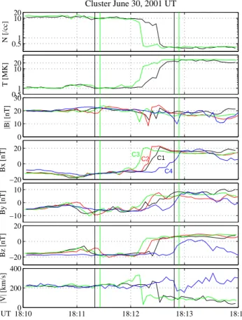
0.51 10 20 N [/cc] Cluster June 30, 2001 UT 0.51 10 20 T [MK] 0 10 20 30 |B| [nT] −20 0 20 Bx [nT] C1 C2 C3 C4 −10 0 10 By [nT] −20 0 20 Bz [nT] 18:100 18:11 18:12 18:13 18:14 200 400 |V| [km/s] UT
Fig. 1. Time series of Cluster measurements around a magne-topause crossing event occurring at (−7.89, −17.11, 3.25) RE in GSE on 30 June 2001. The panels, from top to bottom, show ion number density, ion temperature, intensity and three components of the magnetic field in GSE coordinates, and ion bulk speed, respec-tively (black: spacecraft 1 (C1), red: C2, green: C3, blue: C4). The interval enclosed by the two black vertical lines is used in the recon-struction based on C1 data, while that enclosed by the green lines is in the reconstruction based on C3 data.
2 Cluster event on 30 June 2001, 18:12 UT
2.1 Background information
We utilize data from the Cluster Ion Spectrometry (CIS) and the Flux Gate Magnetometer (FGM) instruments. The CIS instruments measure full 3-D ion distribution functions and moments (R`eme et al., 2001), with a resolution up to the spin rate (∼4 s). The FGM experiment can provide magnetic field measurements at time resolutions up to 120 vector samples/s (Balogh et al., 2001), but only spin-averaged data with ∼4-s time resolution are used throughout this study. For our two events, the CIS instruments were fully operational on space-craft 1 and 3 (C1 and C3). Additionally, after appropriate re-calibration, the CODIF portion of CIS on board C4 delivered reliable velocity measurements. The FGM instruments on all four spacecraft were operating for the two events. However, since the reconstruction requires reliable pressure measure-ments, field maps can be produced only from C1 and C3.
On 30 June 2001, around 18:12 UT, the Cluster spacecraft were moving from northern high-latitude regions toward the
−0.050 0 0.05 0.05 0.1 0.15 0.2 0.25 0.3 0.35 0.4 0.45 0.5 A [T⋅m] Pt = (p + B z 2 /2 µ0 ) [nPa] Cluster−1 June 30, 2001 181120−181249 UT
Fig. 2. Plot of transverse pressure Pt versus computed vector
po-tential A and the fitting curves for the C1 magnetopause cross-ing on 30 June 2001. The circles and stars are data used in pro-ducing the magnetosheath (black curve) and magnetospheric (gray curve) branches, respectively. Extrapolated parts for each branch are shown; these are outside the measurements but are required for the reconstruction.
tail flank on the dawn side. An inbound, complete crossing of the magnetopause occurred when the reference spacecraft (C3) was located at (X, Y, Z)∼(−7.89, −17.11, 3.25) RE in
the GSE coordinate system. Shown in Fig. 1 are, from top to bottom, time plots of ion number density, ion tempera-ture, magnitude and three components of the magnetic field in GSE, and ion bulk speed, respectively. The black, red, green, and blue lines represent the measurements by C1, C2, C3, and C4, respectively. Plasma data for C1 and C3 are pro-vided by the CIS/HIA instrument, which detects ions without mass discrimination. The velocity data for H+ions are pro-vided by the CIS/CODIF instrument on board C4. The figure shows that the Cluster spacecraft were in the magnetosheath, which is characterized by high density (N ∼10 cm−3) and low temperature (T ∼1 MK), until ∼18:12 UT, although sig-natures associated with a flux transfer event (FTE), such as magnetic field perturbations and a temperature enhance-ment (for a review, see Elphic, 1995), were found at around 18:11 UT. The local magnetosheath magnetic field was tail-ward/dawnward/southward. The spacecraft then crossed the magnetopause and entered the plasma sheet where the tem-perature is much higher (∼20 MK) and, in this event, the field magnitude is slightly smaller than in the magnetosheath. The orientation changes of the magnetic field indicate that the time order of the magnetopause traversals was C3, C2, C1, and C4.
We used the following criteria when selecting this cross-ing as a good test case: (1) The slope of the regression line in the Wal´en plot (e.g. Khrabrov and Sonnerup, 1998) is small, indicating strongly subalfv´enic flow in the HT frame. This means that the boundary encountered is likely to be TD-like rather than RD-TD-like, and that inertia effects associated
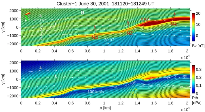
0 0.2 0.4 0.6 0.8 1 1.2 1.4 1.6 1.8 2 x 10⁴ −2000 −1000 0 1000 2000 y [km]
Cluster−1 June 30, 2001 181120−181249 UT
20 nTN1
N2
N3
N4
B
1 2 3 4 [nT] Bz 0 10 20 0 0.2 0.4 0.6 0.8 1 1.2 1.4 1.6 1.8 2 x 10⁴ −2000 −1000 0 1000 2000 x [km] y [km] 100 km/s 1 3 4 Pth [nPa] −V HTx 0 0.1 0.2 0.3Fig. 3. Magnetic transect (top) and plasma pressure distribution (bottom) obtained by using time-varying HT frame velocity for the C1 magnetopause crossing on 30 June 2001. Contours describe the transverse magnetic field lines. In this reconstruction plane, the spacecraft generally moved from left to right: The magnetosheath, where Bx<0; By<0, is on the upper left side and the magnetosphere (Bx>0; By>0)
on the lower right side. In the top panel, Bzis expressed in color as indicated by the color bar; the four spacecraft tetrahedron configuration is
shown by white lines; the measured magnetic field vectors are projected as white arrows along the spacecraft trajectories; the normal vectors, N1 - N4, computed from MVABC, are projected as red arrows. Line segments in the upper left corner are projections of GSE unit vectors,
X(red), Y (green), and Z (yellow), onto the x–y plane. In the bottom panel, the plasma pressure is shown in color; the ion bulk velocity vectors from CIS/HIA (C1 and C3) or CIS/CODIF (C4), transformed into the accelerating HT frame, are projected as white arrows.
with field-aligned plasma flows can be neglected. (2) A good deHoffmann-Teller frame with a constant HT velocity is found. This indicates that motion and time evolution of the structures are negligibly small in the HT frame and also that the MHD frozen-in condition is well satisfied. (3) The speed of the boundary motion along n, calculated, for example, as VH T·n, is small enough to give a sufficient number of
mea-surements within the magnetopause current layer, so as to allow for a good functional fitting of Pt(A)and accurate
re-covery of meso-scale current sheet structures. These criteria can be used for identifying events for which the model as-sumptions are likely to hold and which are therefore suitable for the reconstruction analysis.
The time interval between the two black vertical lines is used for reconstruction from C1 data, whereas that between the green lines in the figure is for reconstruction from C3. These intervals include a number of data samples in both the magnetosheath and in the magnetosphere. Their start times are chosen such that variations related to the FTE are outside the intervals. The reason for this choice is that temporal variations and/or inertia effects, which cannot be taken into account in the current technique, could be signif-icant in the FTE structures. We assume in this study that only ions, assumed to be protons with isotropic temperature, T = (2T⊥+Tk)/3, contribute to the plasma pressure.
2.2 Reconstruction from spacecraft 1 crossing
For the magnetopause encountered by C1, the Wal´en slope (slope of the regression line in a scatter plot of the veloc-ity components in the HT frame, V −VH T, versus the
cor-responding components of the Alfv´en velocity, B/√µ0ρ) is 0.3430. The slope is much smaller than unity, indicat-ing small field-aligned velocities in the HT frame, a result that is consistent with a TD. The minimum variance analysis (e.g. Sonnerup and Scheible, 1998) of the magnetic fields, measured by C1 in the interval 18:12:00–18:12:49 UT and using the constraint hBni=0, (referred to as MVABC,
here-inafter) yields the magnetopause normal vector, n=(0.2003, −0.9654, 0.1671) in GSE. For this crossing and through-out this paper, we use the variance analysis with this con-straint, because, for all the crossings examined in this study, the analysis without the constraint results in a rather small ratio of the intermediate to minimum eigenvalues (< 5)so that the normal determined may not be reliable. The us-age of the constraint is justified for this event, since the Wal´en test shows consistency with a TD. The HT analysis for the same interval results in a constant HT frame velocity, VH T=(−236.6, −83.9, −8.5) km/s, with the correlation
co-efficient between the components of −V ×B from the set of discrete measurements and the corresponding component of
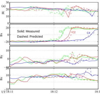
0 10 20 30 |B| (a) −20 0 20 Bx Solid: Measured Dashed: Predicted C2 C3 C4 −10 0 10 By 18:11 18:12 18:13 −10 0 10 20 Bz UT −30 −20 −10 0 10 20 30 −30 −20 −10 0 10 20 30
Bi (Predicted) [nT] i=x,y,z for C2,3,4
Bi (Measured) [nT] i=x,y,z for C2,3,4
Correlation between Measured and Predicted B (B map from SC1)
cc = 0.97905 (b) Bx(C2) By(C2) Bz(C2) Bx(C3) By(C3) Bz(C3) Bx(C4) By(C4) Bz(C4)
Fig. 4. (a) Time series of intensity and three components of the measured (solid) and predicted (dashed) magnetic field data (nT) in the reconstruction coordinates. The predicted data are based on the field map recovered from the C1 data (Fig. 3). (b) Correlation between the measured and predicted magnetic field components. The x, y, and z components in the reconstruction coordinates are represented as a plus, a cross, and a circle, respectively. The curves and points are color-coded as in Fig. 1.
−VH T×B being ccH T=0.9753, indicating that a relatively
good deHoffmann-Teller frame was found for this boundary (the value ccH T=1 corresponds to an ideal HT frame). The
magnetopause motion along n is VH T·n=+32.2 km/s. The
positive sign indicates outward magnetopause motion as ex-pected for an inbound crossing.
By following the procedure described in Appendix A, the orientation of the optimal invariant axis was found to be
ˆ
z=(0.5941, −0.1160, −0.7960) in GSE. Figure 2 shows the resulting data points of Ptversus A, obtained from the
space-craft measurements and the corresponding fitting curves for two separate branches. In constructing the diagram, we have used a slightly modified reconstruction technique in which the use of a sliding-window HT calculation is incorporated so as to allow for temporal variations in the velocity of the mag-netopause structures as they move past the spacecraft (Hu and Sonnerup, 2003); the reason for this procedure will be mentioned later. The sliding-window HT analysis yields a set of HT frame velocities, { ˜VH T}, one vector for each data
point sampled during the analysis interval. The ˜VH T vectors vary from point to point along the spacecraft trajectory, re-sulting in a curved spacecraft trajectory in the reconstruction (x–y) plane. The calculation of the magnetic potential A is then modified to a line integral along the curved trajectory, A = Z ∂A ∂xdx + Z ∂A ∂ydy = Z −By{− ˜VH T} ·xdt +ˆ Z Bx{− ˜VH T} ·ydt.ˆ (3)
The black curve in Fig. 2 is the magnetosheath branch of Pt(A), fitted by a high-order polynomial to the data samples
(open circles) in the magnetosheath and in the central current sheet, a region of intense axial current density (large slope of Pt(A)). The gray curve, fitted to the data samples (stars)
obtained on the magnetospheric side, is the magnetosphere branch of Pt(A). Exponential functions, attached beyond the
measured A range, are used to generate the field map in re-gions of the x–y plane containing field lines that are not en-countered along the trajectory. We describe a reasonable way to determine the extrapolating functions in Appendix A.
The recovered magnetopause transect and the plasma pres-sure distribution are shown in Fig. 3. An improved numerical scheme, developed by Hu and Sonnerup (2003), was used to suppress numerical instabilities and hence, to extend the computation domain in the y direction. The spatial extent in the x direction corresponds to the analysis interval marked in Fig. 1. The spacecraft were moving to the right, as shown in the upper reconstruction map. C2, C3, and C4 were lo-cated away from C1 by −1468 km, +369 km, and +27 km, respectively, in the out-of-plane (z) direction. The contours show the transverse magnetic field lines, Bt=Bxx+Bˆ yy, sep-ˆ
arated by equal flux; color filled contours show the Bz(upper
panel) and p (lower panel) distributions, as specified by the color bars. The white arrows along the spacecraft trajectories in the upper panel show the measured magnetic field vectors, projected onto the x–y plane. The recovered field lines are exactly parallel to these vectors at C1 and also approximately parallel at the locations of the other spacecraft (C2, C3, and C4). The magnetosheath is located on the upper left side, where Bx<0 and By<0, while the magnetosphere is on the
lower right side, where Bx>0 and By>0. The magnetopause
encountered is found to be a thin, markedly nonplanar cur-rent layer of the TD-type. The presence of an X point is ev-ident at (x, y) ≈(13 500.0) km, resulting in a small number
−3000 −2000 −1000 0 1000 2000 3000 y [km] Cluster−3 June 30, 2001 181125−181255 UT 20 nT N3 N1 N2 N4 B 4 1 2 3 [nT] Bz −5 0 5 10 15 20 0 0.2 0.4 0.6 0.8 1 1.2 1.4 1.6 1.8 2 x 10⁴ −3000 −2000 −1000 0 1000 2000 3000 x [km] y [km] 100 km/s 4 1 3 Pth [nPa] −V HTx 0 0.1 0.2 0.3
Fig. 5. Magnetic transect (top) and plasma pressure distribution (bottom) recovered by using a time-varying HT frame velocity for the C3 magnetopause crossing on 30 June 2001. The format and the spatial scale size are the same as in Fig. 3.
of interconnected field lines, embedded in the TD, and pre-sumably in a localized thickening of the current sheet on the right of the X point. The red arrows show the normal vectors computed from MVABC, based on each spacecraft measure-ment, and projected onto the x–y plane. These normal direc-tions are qualitatively consistent with the overall orientation of the recovered magnetopause surface but individual nor-mals can deviate substantially from the local orientation (for example, see the normal for C2). The lower panel shows that the plasma pressure had a maximum in the central current layer. The white arrows in this panel represent the projection of the flow velocity vectors, as seen in the time-dependent HT frame. With a few exceptions, the vectors are approx-imately field-aligned for all three spacecraft, as they ideally should be. The velocities in the co-moving frame are not very large on the magnetosheath side, whereas they have substan-tial values on the magnetosphere side. Thus the HT frame moves approximately with the magnetosheath flow. How-ever, the larger speeds in the magnetosphere contribute lit-tle to inertia forces because the corresponding streamlines, which ideally would coincide with the field lines, have no significant curvature.
Figure 4a shows the comparison between the time series of measured magnitude and the three components along the reconstruction coordinates of the magnetic field, and the cor-responding values computed from the map recovered from C1. The predicted values were obtained along the trajecto-ries of C2, C3, and C4 in Fig. 3. The time scale of the panel is
expanded, relative to Fig. 1, to cover only the reconstructed range. We see that the recovered variations agree qualita-tively with the measured variations for almost the whole in-terval. The recovered values predict the timings of the mag-netopause crossings at the other spacecraft rather well, al-though the durations of the current layer traversals have small differences. Figure 4b illustrates that a very good corre-lation exists between the measured and predicted magnetic field values for C2, C3, and C4: the correlation coefficient is cc = 0.979. This result indicates that the reconstruction technique based on C1 data is rather successful in predicting quantitatively reasonable values at the locations of the other three spacecraft.
The magnitude of this correlation coefficient can be used as a measure for judging whether or not the orientation of the invariant z-axis, the co-moving (HT) frame velocity, and the extrapolating exponential functions in the Pt versus A
plot, are adequately selected. In fact, the optimal invariant axis, the HT frame, and the functional form Pt(A)for the
extrapolated parts are all determined in such a way that the correlation between measured and predicted magnetic field data is at, or near, a maximum. The steps we have used for optimal selection of the invariant axis, the HT frame, and the extrapolating functions are presented in Appendix A.
For the reconstruction in Fig. 3, the results were found to improve by use of the sliding-window HT method, sug-gesting that the whole set of magnetopause structures was approximately time-independent but was moving with small
0 10 20 30 |B| (a) −20 0 20 Bx Solid: Measured Dashed: Predicted C1 C2 C4 −10 0 10 By 18:11 18:12 18:13 −10 0 10 20 Bz UT −30 −20 −10 0 10 20 30 −30 −20 −10 0 10 20 30
Bi (Predicted) [nT] i=x,y,z for C1,2,4
Bi (Measured) [nT] i=x,y,z for C1,2,4
Correlation between Measured and Predicted B (B map from SC3)
cc = 0.9799 (b) Bx(C1) By(C1) Bz(C1) Bx(C2) By(C2) Bz(C2) Bx(C4) By(C4) Bz(C4)
Fig. 6. (a) Time series of the measured (solid) and predicted (dashed) magnetic field data. The predicted data are based on the field map reconstructed from C3 data (Fig. 5). (b) Correlation be-tween the measured and predicted magnetic field data. The format is the same as in Fig. 4.
acceleration. The extended reconstruction technique, devel-oped by Hu and Sonnerup (2003), was shown to be useful for this case. The orientation of the selected invariant axis (z-axis in Fig. 3) corresponds to the angles (defined in Ap-pendix A) θ =−1◦and φ=6◦, i.e. it was rotated away from
the intermediate variance direction by ∼6◦, with the axis of rotation mainly being the maximum variance direction (see Appendix B for a method to determine the intermediate and maximum variance directions under the constraint hBni=0).
2.3 Reconstruction from spacecraft 3 crossing
The reconstruction technique is now applied to the magne-topause traversal by C3 which crossed the boundary ∼20 s earlier than C1 did, using the data interval denoted by two
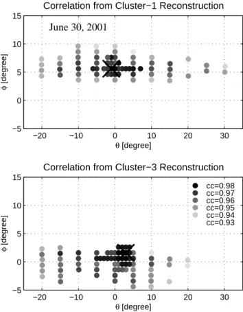
−20 −10 0 10 20 30 −5 0 5 10 15 θ [degree] φ [degree]
Correlation from Cluster−1 Reconstruction
June 30, 2001 −20 −10 0 10 20 30 −5 0 5 10 15 cc=0.93 cc=0.94 cc=0.95 cc=0.96 cc=0.97 cc=0.98 θ [degree] φ [degree]
Correlation from Cluster−3 Reconstruction
Fig. 7. Dependence of the correlation coefficient between the mea-sured and predicted field data on the choice of the invariant (z)-axis for the reconstructions based on the C1 (upper panel) and C3 (lower panel) data; see text for definition of the angles θ and φ. (θ , φ)=(0, 0) corresponds to the intermediate variance direction determined by MVABC for the C1 magnetopause crossing. The orientations of the invariant axes used in producing Figs. 3 and 5 are shown as thick crosses. Note that the vertical and horizontal scales are different.
vertical green lines in Fig. 1. The MVABC and HT anal-ysis yield: n=(0.2117, −0.9608, 0.1791); a constant HT velocity, VH T=(−269.4, −98.3, −14.8) km/s, from the
in-terval 18:11:41–18:12:38 UT. The correlation coefficient is ccH T=0.9598, and VH T·n=+34.7 km/s. The Wal´en slope
is 0.3689, indicating again that inertia effects due to field-aligned flow were reasonably small. As before, these results are consistent with the spacecraft crossing an outward mov-ing magnetopause of the TD-type.
For this case, the reconstruction, using neither the stan-dard (constant HT frame speed) nor the sliding-window HT analysis, led to a satisfactory correlation between the pdicted and measured magnetic field components. These re-sults, and also the fact that the HT frame was less well deter-mined (ccH T=0.9598), suggest that the motion of the
struc-tures varied rapidly and by significant amounts along the C3 trajectory. Therefore, before the reconstruction was per-formed, we modified the y component (in the reconstruction plane) of the HT velocity vectors computed from the sliding-window HT method, such that the remaining velocity vec-tors became completely parallel to the local magnetic field
measured along the spacecraft (C3) trajectory in the recon-struction plane. The obtained Pt(A)profile (not shown) is
qualitatively similar to that for the C1 reconstruction: Pt(A)
has two branches and has smaller values at smaller A, but it generally increases with A and the two branches merge in the largest A range. The magnetic field and pressure maps thus recovered are shown in Fig. 5. The trajectories of the spacecraft are more strongly bent than in Fig. 3, because of the substantial modification of the y component of VH T
needed at certain points. By definition, the alignment be-tween the flow vectors and the transverse field lines is now fulfilled for C3. The invariant axis is found to be z=(0.6261, −0.0246, −0.7794) in GSE which is obtained by rotating the intermediate variance (M) axis, computed from the C1 data, by θ =3◦ and φ=2◦. Thus, this orientation has an angle of 5.6◦ with respect to the invariant axis used in Fig. 3,
indi-cating that the two axes are not far away from one another. As in the previous case (Fig. 3), a qualitative agreement of the normal vectors from MVABC with the orientation of the recovered magnetopause is seen in Fig. 5. Interestingly, the global shape of the magnetopause surface is similar in the two maps - the one from C1 (Fig. 3) and the one from C3 (Fig. 5). The X point, seen in Fig. 3 at x=13 500 km, seems to be equivalent to the one found at (x, y)≈(11 500.0) km in Fig. 5, although its location in y is displaced: it is between the C1 and C2 trajectories in Fig. 3, and between C2 and C3 in Fig. 5. If our interpretation is correct, the migration distance of the X point of about 2000 km during the ∼20-s time interval between the C3 and C1 crossings gives a sun-ward speed of the X point of about 100 km/s in the recon-struction plane. However, that plane was moving downtail at speed VH T·x≈230 km/s. Therefore, relative to Earth, theˆ
X point was sliding tailward at some 130 km/s. The pres-ence of the bulge in the magnetopause seen in Fig. 3 but absent in Fig. 5, may indicate a minor time evolution: it may have been produced as a result of ongoing reconnec-tion activity at the X point. The current layer thickness ap-pears to be somewhat different. A small magnetic island lo-cated at (x, y)≈(9500.0) km in Fig. 5, where both the Bzand
the plasma pressure reach maximum values, is not found in Fig. 3. These differences in fine structures are due to the fact that the profile of the function Pt(A)was quantitatively
different, in and near the current sheet, for C1 and C3 (not shown), i.e. it may have been different on opposite sides of the dominant X point. The structures in the current layer on the left side of the X point in Fig. 5, where the field lines were not encountered by C1, thus may not have been recov-ered correctly in Fig. 3.
The time series of the measured magnetic field magni-tude and components and the corresponding predicted values shown in Fig. 6a indicate that the reconstruction results pre-dict both the timings and durations of the current layer cross-ing very well. In Fig. 5, C1, C2, and C4 were separated from C3 by −325 km, −1848 km, and −480 km, respectively, in the z direction. It is noteworthy that the predicted and mea-sured variations are quite similar even for C2, whose z po-sition was farthest from C3, supporting the conclusion that
the approximate invariance along the selected invariant (z)-axis held over the spatial scale of at least 2000 km. Figure 6b shows that an excellent correlation (cc=0.980) between the measured and predicted field components is attained for this case, demonstrating that the technique succeeds in predicting the conditions in regions surrounding the spacecraft trajec-tory with reasonable accuracy.
2.4 Orientation of invariant axis
Figure 7 shows the dependence of the correlation between the measured and predicted field components on the choice of the invariant (z)-axis. θ and φ are the angles described in Appendix A: (θ , φ)=(−90, 0), (0, 0), and (0, 90) correspond to the maximum, intermediate, and minimum variance direc-tions, respectively, for the C1 magnetopause crossing. The intermediate variance direction computed from the C3 data is oriented toward (θ , φ)≈(2, −1). The correlation coefficient is shown by the darkness of the grey points. The thick cross represents the orientation of the optimal invariant axis used in Figs. 3 and 5. The spaces in the diagram where no points are shown correspond to axis orientations for which an unre-alistic field map is recovered, either due to an unreasonable profile in the Pt versus A plot, or to the correlation
coeffi-cient being smaller than 0.93. The optimal invariant axis is found to be relatively close to the intermediate variance axis, for both the C1 and the C3 reconstructions. The correlation coefficient is sensitive to changes in φ (rotation about the maximum variance direction) but less sensitive to changes in θ(rotation about the minimum variance direction), for both cases. In other words, the magnetic field configuration in the reconstructed map is strongly modified by changes in φ while it is only weakly sensitive to changes in θ , the latter result being the finding also reported by Hau and Sonnerup (1999) and Hu and Sonnerup (2003).
2.5 Summary of 30 June 2001 event
Intercomparison of the two reconstructed maps (Figs. 3 and 5) demonstrates that the magnetopause encountered in this event was a quasi-static, TD-type current layer, for which the model assumptions appear to be well justified. Similarities of the orientation of the invariant axis, current sheet thickness, and the overall magnetopause structures among the results from C1 and C3 data indicate that mainly two-dimensional structures were present, with superimposed weak three-dimensionality and temporal variations. The dominant X point in the two maps appears to be a real feature, mov-ing tailward, relative to Earth, at about 130 km/s. The as-sociated magnetic topology allows for easy access of the magnetosheath plasma to the inner portion of the magne-topause layer, by means of field-aligned flow on the two sides of the X.
3 Cluster event on 5 July 2001, 06:23 UT
3.1 Background information
The second event is a crossing from the magnetosphere to the magnetosheath occurring on 5 July 2001, around 06:23 UT, when C3 was located at ∼(−6.78, −14.97, 6.24) RE in
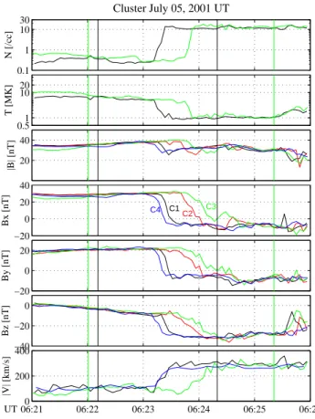
GSE. This event has also been investigated in detail by Haa-land et al. (2004), with the objective of comparing single-and multi-spacecraft determinations of magnetopause orien-tation, speed, and thickness. Time plots of number density, temperature, magnitude and three GSE components of the magnetic field, and bulk flow speed are shown in Fig. 8. Compared to the 30 June event, the spacecraft resided in a higher-latitude part of the plasma sheet before the crossing, as is inferred from the fact that both the magnitude and the x component of the magnetic field were more intense and the temperature was lower than in the 30 June event. The space-craft traversals of the magnetopause took place in the time order C4, C1, C2, and C3, i.e. opposite to the order in the previous event. We see that the duration of the current layer traversal was relatively short for C4 and C1, whereas it was longer for C2 and C3. The local magnetosheath magnetic field was tailward/dawnward/southward, as in the previous event.
3.2 Reconstruction from spacecraft 1 crossing
The MVABC and HT analysis for the interval 06:23:03– 06:23:44 UT yield (all vectors are in GSE): the mag-netopause normal vector, n=(0.6098, −0.7862, 0.0999); the constant HT frame velocity, VH T=(−248.6, −102.5,
68.6) km/s with the correlation coefficient, ccH T=0.9660
(These two vectors are very close to, but not identical to those reported in Haaland et al. (2004)). The usage of the constraint hBni=0 might be questionable for this event, since,
as shown later, the Wal´en relation is relatively well satisfied, i.e. the boundary may be of the rotational discontinuity-type. Nonetheless, we use the constraint because the orientation of the normal with, rather than without, the constraint is more consistent with those from various other methods (Haaland et al., 2004). Also the result without the constraint leads to an unlikely large Bn value. The normal component of
the HT velocity is negative (VH T·n=−64.1 km/s),
consis-tent with an outbound crossing of the magnetopause. The field map recovered from the C1 measurements during the time interval of 06:22:11 to 06:24:20 UT is shown in Fig. 9. For this event, the constant HT velocity is used for the re-construction, because effects other than the kinematic ef-fects of HT frame acceleration could be substantial, as will be shown later in this section. The optimal invariant axis is found to be z=(0.6066, 0.3061, −0.7337) (GSE) and C2, C3, and C4 were displaced from C1 by −1219 km, +935 km, and −570 km, respectively, in the z direction. In the recon-struction plane, the magnetosphere (Bx>0; By<0) is on the
lower left side and the magnetosheath (Bx<0; By>0) on the
upper right side. The magnetopause appears to be a slightly
0.1 1 10 30 N [/cc] Cluster July 05, 2001 UT 0.51 10 20 T [MK] 20 40 |B| [nT] −20 0 20 40 Bx [nT] C1 C2 C3 C4 −20 0 20 By [nT] −40 −20 0 Bz [nT] 06:210 06:22 06:23 06:24 06:25 06:26 200 400 |V| [km/s] UT
Fig. 8. Time plots of Cluster measurements around a magnetopause crossing event occurring at (−6.78, −14.97, 6.24) REin GSE on 5 July 2001. The format is the same as in Fig. 1.
bent TD-like structure. Thinning of the current sheet locally at (x, y) ≈(9000, 1000) km implies the presence of an X point at this location. The flow velocities remaining in the HT frame are shown by the white arrows. They are negligi-bly small on the magnetosheath side, indicating that, as be-fore, the HT frame is strongly anchored in the magnetosheath plasma. Near the magnetopause on its magnetospheric side, the flow directions in the C1 and C3 crossings are consistent with the recovered field configuration. The yellow arrows, representing the normal vectors determined from MVABC for each spacecraft measurement are approximately perpen-dicular to the recovered magnetopause surface.
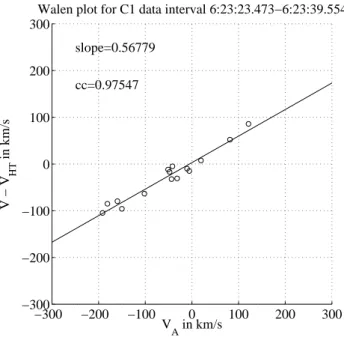
Figure 10 shows the result of the Wal´en test across the C1 magnetopause crossing, in which GSE velocity components in the HT frame are plotted against the corresponding com-ponents of the Alfv´en velocity. The regression line has a sig-nificant positive slope (slope=0.568), suggesting that some reconnection activity could have been present. The positive slope means that the plasma was flowing parallel to the field, which has a small negative normal component, Bn, at the
lo-cation of C1. In other words, one may infer that plasma was flowing earthward across the magnetopause, albeit at consid-erably less than Alfv´enic speeds. These results are consistent with the reconstructed field map, although the C1 velocity vectors shown in the map do not show clear direct evidence for such an earthward flow component.
0 2000 4000 6000 8000 10000 12000 14000 16000 18000 −1000 0 1000 x [km] y [km] Cluster−1 July 05, 2001 062211−062420 UT 100 km/s 1 2 3 4 N1 N2 N3 N4 B [nT] Bz −V HTx 0 20 40
Fig. 9. Magnetic field map reconstructed by using a constant HT velocity for the C1 magnetopause crossing on 5 July 2001. The format is the same as in the upper panel of Fig. 3, except that for C1, C3, and C4, the flow vectors in the HT frame are projected as white arrows, and for C2, the spacecraft trajectory is shown by a white curve. In this plane the magnetotail (Bx>0; By<0) is on the lower left side, whereas
the magnetosheath (Bx<0; By>0) is on the upper right side. The yellow arrows show the projections of the normal vectors determined from
MVABC. −300 −200 −100 0 100 200 300 −300 −200 −100 0 100 200 300 V A in km/s V − V HT in km/s
Walen plot for C1 data interval 6:23:23.473−6:23:39.554 slope=0.56779
cc=0.97547
Fig. 10. Wal´en relation across the magnetopause encountered by C1 at 06:23 UT on 5 July 2001. VH T=(−242.65, −84.71,
162.28) km/s in GSE.
In Fig. 11 the correlation between the field components measured by C2, C3, and C4 and the corresponding com-ponents predicted from the reconstruction map (Fig. 9) are shown. The correlation is slightly lower than in the previous event but it remains high, demonstrating that the reconstruc-tion technique works well also for this case. A few outlying points from the Bx component of the C4 data result from a
small error in the predicted time of the crossing by C4.
−40 −20 0 20 40 −40 −30 −20 −10 0 10 20 30 40
Bi (Predicted) [nT] i=x,y,z for C2,3,4
Bi (Measured) [nT] i=x,y,z for C2,3,4
Correlation between Measured and Predicted B (B map from SC1)
cc = 0.97049 Bx(C2) By(C2) Bz(C2) Bx(C3) By(C3) Bz(C3) Bx(C4) By(C4) Bz(C4)
Fig. 11. Correlation between the measured and predicted magnetic field data. The predicted data are from the field map recovered for the C1 traversal on 5 July 2001 (Fig. 9).
3.3 Reconstruction from spacecraft 3 crossing
The MVABC and HT analysis for the interval 06:23:32– 06:24:49 UT yield: n=(0.5959, −0.8000, 0.0704); the constant HT frame velocity, VH T=(−236.0, −94.5,
125.4) km/s with the correlation coefficient, ccH T=0.9512;
and VH T·n=−56.2 km/s. The GSE z component of the HT
velocity is substantially different from that computed for the C1 traversal; a possible explanation will be mentioned later. The normal motion of the magnetopause is negative, i.e. earthward, as required, although Haaland et al. (2004) have shown from Minimum Faraday Residue (MFR) analysis that the inward magnetopause speed was only some 43 km/s.
0
2000
4000
6000
8000
10000
12000
−1000
0
1000
2000
3000
4000
5000
x [km]
y [km]
Cluster−3 July 05, 2001 062200−062521 UT
4
1
2
3
N1
N3
N2
N4
B
100 km/s
[nT]
Bz
−V
HTx0
10
20
30
40
Fig. 12. Magnetic field map reconstructed for the C3 magnetopause crossing on 5 July 2001. The format is the same as in Fig. 9, except that the normal vectors are shown as red arrows.
−300 −200 −100 0 100 200 300 −300 −200 −100 0 100 200 300 V A in km/s V − V HT in km/s
Walen plot for C3 data interval 6:23:52.716−6:24:36.79 slope=1.0273
cc=0.97947
Fig. 13. Wal´en relation for the C3 magnetopause crossing oc-curring at 06:24 UT on 5 July 2001. VH T=(−254.11, −95.92,
225.78) km/s in GSE. The Wal´en slope close to +1 is consistent with a rotational discontinuity magnetopause, with the magnetic field having an inward component.
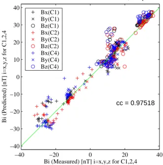
−40 −20 0 20 40 −40 −30 −20 −10 0 10 20 30 40
Bi (Predicted) [nT] i=x,y,z for C1,2,4
Bi (Measured) [nT] i=x,y,z for C1,2,4
Correlation between Measured and Predicted B (B map from SC3)
cc = 0.97518 Bx(C1) By(C1) Bz(C1) Bx(C2) By(C2) Bz(C2) Bx(C4) By(C4) Bz(C4)
Fig. 14. Correlation between measured and predicted magnetic field data. The predicted data are based on the map reconstructed from the C3 data for the 5 July 2001 event (Fig. 12).
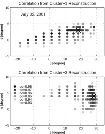
−20 −10 0 10 20 30 −5 0 5 10 θ [degree] φ [degree]
Correlation from Cluster−1 Reconstruction July 05, 2001 −20 −10 0 10 20 30 −5 0 5 10 cc=0.93 cc=0.94 cc=0.95 cc=0.96 cc=0.97 cc=0.98 θ [degree] φ [degree]
Correlation from Cluster−3 Reconstruction
Fig. 15. Dependence of the correlation coefficient on the choice of the invariant axis for the reconstructions from the C1 (upper panel) and C3 (lower) traversals on 5 July 2001. The format is the same as in Fig. 7.
The difference between this number and 56.2 km/s indicates the presence of an inward flow of plasma across the mag-netopause. The magnetic field map reconstructed for this C3 magnetopause crossing, using the data from 06:22:00 to 06:25:21 UT, is shown in Fig. 12. The selected optimal in-variant axis is z=(0.6997, 0.3727, −0.6096) (GSE), which is tilted from the invariant axis used in Fig. 9 by 9.7◦. A sig-nificant amount of field lines that connect the magnetosheath and magnetospheric sides of the magnetopause is seen in the map. A prominent X point in the transverse field at (x, y)≈ (4000, 3000) km looks more like a Y point. The HT frame is no longer anchored in the magnetosheath plasma, i.e. the flow vectors have substantial field-aligned components in the magnetosheath. This behavior is suggestive of ongoing re-connection. Note that the plasma is flowing across the mag-netopause in the direction parallel to the magnetic field in the open-field channel between the X point and the center of a bulge in the current layer, located at (x, y)≈ (7500, 0) km, indicating that the magnetosheath plasma enters the magne-tosphere along the reconnected field lines. The flow vectors have significant downward and rightward components at the bulge center, implying that in the reconstruction frame the reconnected flux tubes were moving in this direction. No-tice that the spatial dimension of the map in the x direction
is smaller than in Fig. 9, in spite of the longer data analysis interval (see Fig. 8). This is due to a smaller HT frame speed along the x-axis for the C3 traversal, caused by the frame motion being better anchored in the reconnected field lines than for the C1 traversal.
The Wal´en plot for the C3 crossing is shown in Fig. 13. The flow speed in the HT frame is almost 100% of the Alfv´en speed, in excellent agreement with the expectation from a one-dimensional RD. For earthward plasma flow across the magnetopause, the positive slope of the regression line im-plies that the normal magnetic field also points inward. This is consistent with the field map and with reconnection occur-ring tailward of the spacecraft. As in the 30 June event, the reconnection site is moving relative to Earth with a tailward velocity component.
Comparison of the two magnetic field maps for this event (Figs. 9 and 12) shows that there was dramatic evolution of the configuration during the 30-s time interval between the traversals by C1 and C3. At the moment when C1 crossed the current layer, there was incipient reconnection, as suggested by the corresponding Wal´en plot (Fig. 10). On the other hand, it is clear that when C3 crossed the magnetopause, the reconnection was fully developed and had resulted in the for-mation of a wide channel of interconnected field lines. The full-blown reconnection caused a localized thickening of the magnetopause current layer in the region traversed by C3 and an associated longer duration of this crossing (see Fig. 8). The crossing by C2 also had a long duration, which may, however, have been the result, at least in part, of a smaller magnetopause speed (Haaland et al., 2004). Such changes in speed are not accommodated by the map, which is based on a constant HT velocity.
Figure 14 shows the same type of correlation plot as Fig. 11, except that the predicted values are based on the map shown in Fig. 12. The correlation (cc=0.975) suggests that the technique predicts conditions at the other three spacecraft locations fairly well. This result may be surprising since the map is derived under the assumption that inertia forces are small, which is not the case near the bulge where the stream-lines have strong curvature and where the flow speed in the HT frame is comparable to the Alfv´en speed (Fig. 13). The assumption that the time dependence of the structures is neg-ligible is also not valid for this event, as is evident from a comparison of the maps in Figs. 9 and 12. Nevertheless, our results indicate that the maps recovered from C1 and C3 are at least qualitatively correct.
3.4 Orientation of invariant axis
In Fig. 15 the dependence of the correlation between the measured and predicted field components on the choice of the invariant (z)-axis for the 5 July 2001, event is shown. In these coordinates, the intermediate variance direction from MVABC is oriented at (θ , φ)=(0, 0) for the C1 crossing, while it is at (θ , φ)≈(2, −1) for the C3 crossing. We also see in this event that the optimal invariant axis is not far from the intermediate variance direction for both reconstructions.
As in the previous event, the reconstruction from the C1 data produces a correlation coefficient that depends strongly on φ but only weakly on θ . This behavior may be understood in the following way. The three reconstructions in Figs. 3, 5, and 9 exhibit a magnetopause current layer that is modestly tilted with respect to the x-axis in the reconstruction plane. Hence, rotations around the minimum variance axis (changes in θ ) change the By component in the reconstruction plane
only weakly, and do not have a significant influence on av-erage profiles of A calculated along the spacecraft trajectory. It follows that the behavior of the function Pt(A)and hence,
the reconstruction result, have only a modest dependence on θ. On the other hand, rotations around the maximum vari-ance axis, i.e. changes in φ, cause significant changes in By
and therefore, a strong dependence on φ.
In contrast, we find the correlation coefficient to be sensi-tive to variations in both θ and φ for the C3 reconstruction on 5 July (see Fig. 12). This behavior may be related to fea-tures that were not seen for the other three cases: The magne-topause crossed by C3 was tilted more steeply, relative to the x-axis, it was of the RD-type, and it had a fairly large-scale 2-D structure, namely the reconnection-associated bulge. A study of more cases is required to determine which of these factors affect the sensitivity of the correlation to variations of the orientation of the z-axis.
3.5 Summary of 5 July 2001 event
Substantial differences in the two recovered maps indicate that the magnetic field configuration evolved dramatically in the ≈30-s interval between the magnetopause crossings by C1 and C3. At the time of the crossing by C1, the mag-netopause was basically a TD-type current layer but with a small amount of interconnected field lines embedded. The boundary crossed by C3 had a much thicker current layer of RD-type. The presence of a single dominant X point and an associated reconnection layer is evident in the field map recovered for the C3 crossing, indicating that reconnection had been developing locally in a time period less than 30 s. Although the model assumptions of time invariance and of negligible inertia forces are violated in the event, the bulge in the magnetopause, containing reconnected field lines in the C3 map, was found to be a persistent feature in our var-ious reconstruction attempts. For this reason, we believe the C3 map to be at least qualitatively correct.
4 Summary and discussion
In this paper, we have applied the technique for recovering 2-D magnetohydrostatic structures from single-spacecraft data to two magnetopause crossings by the four Cluster space-craft, occurring when they were separated by about two thou-sand km from each other. In summary, the following results have been obtained.
1. An optimal invariant (z)-axis can be found in such a way that the correlation between the magnetic field components
predicted from the reconstruction map for one spacecraft and the corresponding components measured by the other three is at, or near, a maximum, with the proviso that the mea-sured velocity vectors, transformed into the co-moving (HT) frame, become nearly field-aligned in the field map (see Ap-pendix A). The orientation of the invariant axis thus selected is relatively close to the intermediate variance direction de-termined by MVABC. The invariant axis is generally well determined with respect to rotations around the maximum variance axis but less well with respect to rotations around the minimum variance axis.
2. Two complete magnetopause crossings, occurring on 30 June 2001 and 5 July 2001, have been examined. For each of the two events, two reconstruction maps have been produced, one based on the data from C1 and a second based on the data from C3. For an optimally selected invariant (z)-axis and HT frame velocity, the correlation coefficient between the predicted and measured field components exceeds 0.97 in all four cases. The result demonstrates that the reconstruction technique is capable of predicting field behavior at distances up to a few thousand km away from the spacecraft used for the reconstruction.
3. The reconstruction method incorporating the sliding-window HT analysis that takes into account time-varying motions of the HT frame, as described by Hu and Sonnerup (2003), was successfully applied to the 30 June 2001 event. This result suggests that, over a spatial scale of a few thou-sand km, the entire portion of the magnetopause shown in a map was approximately time-stationary but was moving in a time-dependent way. Localized motions of the magne-topause were small.
4. Intercomparison of the two field maps obtained for the 30 June 2001 event shows that the overall magnetopause structures were similar in the two maps, having a current layer of TD-type. It appears that the assumptions of local two dimensionality and time coherence were well satisfied for the magnetopause encountered on this day. The recon-structed field structures show a current layer significantly bent on spatial scales of a few thousand km, demonstrating that the magnetopause cannot always be treated as a planar structure during a Cluster encounter. Haaland et al. (2004) have shown that even modest deviations from the planar ge-ometry can lead to difficulties with various multi-spacecraft techniques for predicting the magnetopause velocity.
5. In the 5 July 2001, event, time evolution is clear from comparison of two field maps recovered individually from C1 and C3, which crossed the magnetopause at different mo-ments. Evidence consistent with reconnection developing lo-cally in the magnetopause current layer over a time interval of 30 s or less has been found. The map recovered for C3 shows a rather thick current layer with a dominant X point and interconnected flux tubes embedded, allowing for an ef-ficient access of the magnetosheath plasma into the magne-tosphere, while the map for C1, which spacecraft crossed the boundary ∼30 s earlier than C3 did, shows a thin TD-type current sheet within which a much smaller amount of inter-connected field lines is present.
6. Density ramps at the magnetopause occurred in the earthmost half of the current layer in both events (see Figs. 1 and 8). This behavior is consistent with the recovered field maps which show a dominant X point and associated flux tubes that connect the outer and inner parts of the magne-topause transition layer. The interconnection permits effec-tive transport of magnetosheath plasma into most of the cur-rent layer, via field-aligned flow. The ramps were located in the inner half of the current sheet, for the C1 traversal in the 30 June 2001 event and for the C3 traversal in the 5 July 2001 event, whereas they were closer to the center of the current sheet, for the C3 traversal in the June 30 event, and for the C1 traversal in the 5 July event. This can be explained by the temporal evolutions seen in the maps: for both events, the layer consisting of the interconnected field lines had been thickened during the interval between the C1 and C3 traversals. In neither event is there any evidence of a low-latitude boundary layer, containing magnetosheath-like plasma, earthward of, but adjoining, the magnetopause.
7. Our experiments have shown that the optimal invariant (z)-axis is not far away from the intermediate variance direc-tion for the cases examined, but also that a modest rotadirec-tion of the trial z-axis around the maximum variance direction is critical for optimization of the map. This could be related to the fact that the ratio of intermediate to minimum eigenval-ues is often not very large, resulting in significant uncertain-ties in the determination of both minimum and intermediate variance directions (Sonnerup and Scheible, 1998). Proxim-ity of the invariant axis to the intermediate variance direc-tion suggests that MVABC can provide a rough estimadirec-tion of the orientation of the axis of two-dimensional structures and hence, of X lines, etc.
8. The orientation of the optimal invariant axis is not very different for the two events, which were at positions not-too-distant from one another: The angle between the invari-ant axes for the C1 crossings is ≈25◦. It is also noted that the orientation of the magnetic field outside of the magne-topause was relatively similar among the two events: The angle between the magnetosheath field directions for the 30 June 2001 and 5 July 2001 events is 15◦. This result sug-gests that, at a chosen location on the magnetopause surface, the orientation of the reconnection lines is similar for similar IMF directions. This topic and also the question of how the orientation of the X lines depends on the solar wind condi-tions are important subjects to be pursued in future work by applying the reconstruction method to more events.
9. Both events occurred on the tail flank magnetopause, on the dawn side. The signatures of the RD-type current layer, found for the 5 July 2001 event in both the reconstruction re-sult and the Wal´en test for C3, suggest that reconnection can occur at the dawn tail magnetopause, consistent with the con-clusion reached by Phan et al. (2001). But the local magnetic shear for the 5 July 2001, event was not very high (101◦), in contrast with the reconnection events reported by Gosling et al. (1986) and Phan et al. (2001). Those events also oc-curred at the tail flank magnetopause but under almost an-tiparallel field conditions. The present event is consistent
with the finding that occurrence of reconnection on the tail surface is not rare even for relatively modest magnetic shears (Hirahara et al., 1997; Hasegawa, 2002; Hasegawa et al., 2004). It is noted in Fig. 12 that a clear X point and sig-nificant out-of-plane magnetic field components are found within the reconstructed domain, demonstrating that compo-nent merging was occurring. Our results for the 5 July 2001 event also indicate that the reconnection site was not station-ary relative to Earth but was moving both downstream and toward higher latitudes.
10. Although a qualitatively consistent field map was ob-tained for the C3 crossing on 5 July 2001, the fact that the Wal´en slope was close to one (Fig. 13) indicates that iner-tia forces must have played an important role in the tangen-tial stress balance in the reconnection layer. Incorporation of inertia effects into the reconstruction technique is not sim-ple but is necessary for accurate modeling of magnetopause structures during significant reconnection activity, as on 5 July 2001. If such effects could be accurately taken into ac-count, the recovered field map might show significant quan-titative deviations from the one shown in Fig. 12, at least near the reconnection site. Even so, we expect the map in Fig. 12 to be qualitatively correct. Development and test-ing of a technique that incorporates inertia effects will be ad-dressed in a future study.
11. The present work has made it clear that the past one-dimensional (1-D) local view of the magnetopause is not ad-equate. The constrained normal, n, from MVABC appears to represent the average magnetopause orientation relatively well, but the reconstructed maps show that the local orienta-tions can deviate from the average. Mesoscale 2-D structures seen in the magnetopause current layer and their dependence on parameters on the two sides will provide insights into how reconnection operates and how the mesoscale phenomena are controlled by the plasma parameter regime. These problems will be dealt with in a future statistical study.
Appendix A Optimizing the invariant (z)-axis, HT frame, and extrapolations of Pt(A)
In this Appendix, we describe the steps taken to find an opti-mal invariant axis, HT frame, and extrapolations of the trans-verse pressure function Pt(A). In the present study, we try to
determine the above parameters basically in such a way that the correlation between the measured and predicted magnetic field components becomes higher. This process is justified since, under the model assumptions, variations in time series data measured by the spacecraft should translate directly into spatial variations along the trajectory of spacecraft across static magnetic field structures, i.e. they should be caused by motion of the structures past the spacecraft. We use the reconstruction from C1 on 30 June 2001, at 18:12 UT as a ve-hicle for the presentation but the steps described are general ones.
1. Initially, the HT frame, i.e. the motion of the local struc-tures past the spacecraft, which is required for determination
of the spatial scale of the reconstruction domain in the x di-rection and for computation of the magnetic vector potential, A, is determined. Under the assumption of time indepen-dence of the structures, acceleration or/and rotation of the HT frame is allowed, but as a first step we simply use a con-stant HT frame velocity obtained from C1 for the interval 18:12:00–18:12:49 UT.
2. We define L, M, and N axes as the maximum, in-termediate, and minimum variance directions, respectively, which are determined from MVABC (Appendix B) and are ordered as a right-handed orthogonal coordinate system with N pointing outward. An optimal invariant axis is searched for by rotating the trial z-axis by trial and error, starting from the intermediate variance (M) direction, such that the corre-lation coefficient in Fig. 4b, between the measured and pre-dicted field components, reaches a higher value. First the initial invariant axis (the M axis) is rotated in the plane per-pendicular to N by an angle θ from the M direction. New axes M0 and L0 are determined after this rotation. The trial invariant (M0) axis thus obtained is then rotated by φ in the plane perpendicular to L0, resulting in a new invariant axis M00, which is used for a trial reconstruction. The positive signs of θ and φ are defined according to the right-hand rule. A certain number of candidate orientations, M00, for which the correlation coefficient is sufficiently high, are chosen by surveying the two angles, θ and φ. In principle, any coor-dinate system may be used for this survey process. In this study, we use the coordinate system based on the results from MVABC.
3. As shown in Fig. 7, the angular domain in which the correlation coefficient exceeds a certain value is belt-like and there is an uncertainty in the determination of an optimal θ value. Therefore, two further criteria are used to select the best invariant axis from the candidate orientations, one based on the functional behavior of Pt(A), p(A), and Bz(A), the
other based on the alignment between the remaining veloc-ity vectors in the HT frame and magnetic field lines, when visually inspected in the recovered map. For some of the candidates, the quantities Pt, p, or Bzhave two or more
sig-nificantly different values for certain A values near the center of the current sheet, i.e. near the maximum of Ptand A in the
Ptversus A plot (see Fig. 2), meaning that they vary
substan-tially on the same field line and thus, that the model assump-tions are violated. For other cases, the velocity vectors in the HT frame of C1, measured by the spacecraft not used for the reconstruction (C3 and C4), have non negligible components in the direction perpendicular to the reconstructed magnetic field lines. This feature suggests that the recovered field may not be reasonable. The best orientation of the invariance (z) is determined by considering these features.
4. In a second cycle of trial and error, the reconstruction is tested by incorporating the sliding-window HT technique (Hu and Sonnerup, 2003), which allows for the acceleration of the HT frame. This step is taken unless a very nearly time-independent HT frame is found, that is unless the correlation coefficient between components of −V ×B and −VH T×B
for the analysis interval is extremely good. Note that the
ap-plication of this method assumes that the entire structure en-countered by the four spacecraft moves together with a time-varying HT velocity. Inertia effects associated with the ac-celeration of the HT frame are assumed to be negligible. The optimal invariant axis can then be selected in the same way as in steps 2 and 3. If a better correlation is obtained than for the constant HT velocity case, the result obtained by us-ing the time-varyus-ing HT velocity is adopted as the optimal one. Otherwise, the result with the constant HT velocity is selected.
5. If a less than satisfactory correlation is obtained for both the constant and the time-varying HT velocity cases, a modified method to compute the HT velocity that results in larger acceleration of the HT frame, described in Sect. 2.3, can be tested to improve the result.
6. Our experience indicates that the correlation coefficient depends relatively strongly on the choice of both the invari-ant axis and the HT frame velocity, but only weakly on the behavior of the extrapolating exponential functions in the Pt
versus A plot. Therefore, these exponential functions are ad-justed after the above steps are finished. The above behavior is reasonable, since the extrapolating functions only modify magnetic field values in regions far from the current sheet, but have no effect on the shape of the current sheet. The correlation coefficient seems most sensitive to how well the timing of the magnetopause crossings is predicted.
Appendix B Intermediate and maximum variance axes with the constraint hBni=0
Methods for determining the vector normal to the magne-topause with the constraint hBni=0 were given by Sonnerup
and Scheible (1998). Here we describe a method to deter-mine the intermediate and maximum variance directions un-der this constraint.
By using a constraint of the form ˆn·ˆe=0, where ˆe is a known unit vector (here to be chosen as the normal vector from MVABC, nhBni=0), the eigenvalue problem can be writ-ten,
P · MB·P · ˆn = λ ˆn. (B1)
Here, MB is the magnetic variance matrix, MBij≡hBiBji−hBiihBji, and P is the matrix describing
the projection of a vector onto the plane perpendicular to ˆ
e, i.e. Pij=δij−eiej. By putting ˆn=ˆe in the eigenvalue
Eq. (B1), it is seen that ˆe is an eigenvector corresponding to λ=0. The other two eigenvalues are denoted by λminand λmax. The eigenvectors corresponding to λmin and λmax represent the minimum and maximum variance directions, respectively, in the plane perpendicular to ˆe. Thus, for ˆ
e=nhBni=0, the eigenvectors for λminand λmaxrepresent the intermediate and maximum variance directions, respectively, under the constraint hBni=0. If one puts ˆe=|hBi|hBi instead, the
eigenvector corresponding to λminis the normal vector from MVABC (Sonnerup and Scheible, 1998).