Multi-Criteria Inventory Classification and Root Cause Analysis Based on Logical Analysis of Data

UNIVERSITÉ DE MONTRÉAL

MULTI-CRITERIA INVENTORY CLASSIFICATION AND ROOT CAUSE ANALYSIS BASED ON LOGICAL ANALYSIS OF DATA

YUCHANG WU

DÉPARTEMENT DE MATHÉMATIQUES ET DE GÉNIE INDUSTRIEL ÉCOLE POLYTECHNIQUE DE MONTRÉAL

MÉMOIRE PRÉSENTÉ EN VUE DE L’OBTENTION DU DIPLÔME DE MAÎTRISE ÈS SCIENCES APPLIQUÉES

(GÉNIE INDUSTRIEL) OCTOBRE 2016

UNIVERSITÉ DE MONTRÉAL

ÉCOLE POLYTECHNIQUE DE MONTRÉAL

Ce mémoire intitulé :

MULTI-CRITERIA INVENTORY CLASSIFICATION AND ROOT CAUSE ANALYSIS BASED ON LOGICAL ANALYSIS OF DATA

présenté par : WU Yuchang

en vue de l’obtention du diplôme de : Maîtrise ès sciences appliquées

a été dûment accepté par le jury d’examen constitué de :

M. ADJENGUE Luc-Désiré, Ph. D., président

Mme YACOUT Soumaya, D. Sc., membre et directeur de recherche

DEDICATION

I delicate this thesis to my family for their endless love and support, and friends who helped me in my difficulties and encouraged me to follow my dreams.

ACKNOWLEDGEMENTS

First and foremost, I would like to express my sincere gratitude to my supervisor Professor Soumaya Yacout for her continuous support of my study and related research, for her profound guidance, constructive advice, and immense knowledge. I appreciate her patience and valuable opinion during writing of this thesis. With her confidence in me and support, the thesis is becoming possible. I also want to thank my committee members, Dr. Luc-Désiré Adjengue and Dr. Mohamed-Salah Ouali for serving as my jury committee. Their constructive comments help me refine my thesis.

My gratitude and appreciation goes as well to all those colleagues from our department for their help and advice.

My sincere thanks also go to Jeffrey Mo who encouraged me in any possible way. Without his precious support, it would not be possible to come here to finish my study.

Last but not the least, I would like to thank my family: my parents and my sister for supporting me spiritually throughout the journey of study and my life in general.

RÉSUMÉ

La gestion des stocks de pièces de rechange donne un avantage concurentiel vital dans de nombreuses industries, en passant par les entreprises à forte intensité capitalistique aux entreprises de service. En raison de la quantité élevée d'unités de gestion des stocks (UGS) distinctes, il est presque impossible de contrôler les stocks sur une base unitaire ou de porter la même attention à toutes les pièces. La gestion des stocks de pièces de rechange implique plusieurs intervenants soit les fabricants d'équipement d'origine (FEO), les distributeurs et les clients finaux, ce qui rend la gestion encore plus complexe. Des pièces de rechange critiques mal classées et les ruptures de stocks de pièces critiques ont des conséquences graves. Par conséquent il est essentiel de classifier les stocks de pièces de rechange dans des classes appropriées et d'employer des stratégies de contrôle conformes aux classes respectives. Une classification ABC et certaines techniques de contrôle des stocks sont souvent appliquées pour faciliter la gestion UGS.

La gestion des stocks de pièces de rechange a pour but de fournir des pièces de rechange au moment opportun. La classification des pièces de rechange dans des classes de priorité ou de criticité est le fondement même de la gestion à grande échelle d’un assortiment très varié de pièces. L'objectif de la classification est de classer systématiquement les pièces de rechange en différentes classes et ce en fonction de la similitude des pièces tout en considérant leurs caractéristiques exposées sous forme d'attributs. L'analyse ABC traditionnelle basée sur le principe de Pareto est l'une des techniques les plus couramment utilisées pour la classification. Elle se concentre exclusivement sur la valeur annuelle en dollar et néglige d'autres facteurs importants tels que la fiabilité, les délais et la criticité. Par conséquent l’approche multicritères de classification de l'inventaire (MCIC) est nécessaire afin de répondre à ces exigences.

Nous proposons une technique d'apprentissage machine automatique et l'analyse logique des données (LAD) pour la classification des stocks de pièces de rechange. Le but de cette étude est d'étendre la méthode classique de classification ABC en utilisant une approche MCIC. Profitant de la supériorité du LAD dans les modèles de transparence et de fiabilité, nous utilisons deux exemples numériques pour évaluer l'utilisation potentielle du LAD afin de détecter des contradictions dans la classification de l'inventaire et de la capacité sur MCIC.

Les deux expériences numériques ont démontré que LAD est non seulement capable de classer les stocks mais aussi de détecter et de corriger les observations contradictoires en combinant l’analyse des causes (RCA). La précision du test a été potentiellement amélioré, non seulement par l’utillisation du LAD, mais aussi par d'autres techniques de classification d'apprentissage machine automatique tels que : les réseaux de neurones (ANN), les machines à vecteurs de support (SVM), des k-plus proches voisins (KNN) et Naïve Bayes (NB). Enfin, nous procédons à une analyse statistique afin de confirmer l'amélioration significative de la précision du test pour les nouveaux jeux de données (corrections par LAD) en comparaison aux données d'origine. Ce qui s’avère vrai pour les cinq techniques de classification. Les résultats de l’analyse statistique montrent qu'il n'y a pas eu de différence significative dans la précision du test quant aux cinq techniques de classification utilisées, en comparant les données d’origine avec les nouveaux jeux de données des deux inventaires.

ABSTRACT

Spare parts inventory management plays a vital role in maintaining competitive advantages in many industries, from capital intensive companies to service networks. Due to the massive quantity of distinct Stock Keeping Units (SKUs), it is almost impossible to control inventory by individual item or pay the same attention to all items. Spare parts inventory management involves all parties, from Original Equipment Manufacturer (OEM), to distributors and end customers, which makes this management even more challenging. Wrongly classified critical spare parts and the unavailability of those critical items could have severe consequences. Therefore, it is crucial to classify inventory items into classes and employ appropriate control policies conforming to the respective classes. An ABC classification and certain inventory control techniques are often applied to facilitate SKU management.

Spare parts inventory management intends to provide the right spare parts at the right time. The classification of spare parts into priority or critical classes is the foundation for managing a large-scale and highly diverse assortment of parts. The purpose of classification is to consistently classify spare parts into different classes based on the similarity of items with respect to their characteristics, which are exhibited as attributes. The traditional ABC analysis, based on Pareto's Principle, is one of the most widely used techniques for classification, which concentrates exclusively on annual dollar usage and overlooks other important factors such as reliability, lead time, and criticality. Therefore, multi-criteria inventory classification (MCIC) methods are required to meet these demands.

We propose a pattern-based machine learning technique, the Logical Analysis of Data (LAD), for spare parts inventory classification. The purpose of this study is to expand the classical ABC classification method by using a MCIC approach. Benefiting from the superiority of LAD in pattern transparency and robustness, we use two numerical examples to investigate LAD’s potential usage for detecting inconsistencies in inventory classification and the capability on MCIC.

The two numerical experiments have demonstrated that LAD is not only capable of classifying inventory, but also for detecting and correcting inconsistent observations by combining it with the Root Cause Analysis (RCA) procedure. Test accuracy improves potentially not only with the LAD technique, but also with other major machine learning classification techniques, namely artificial

neural network (ANN), support vector machines (SVM), k-nearest neighbours (KNN) and Naïve Bayes (NB). Finally, we conduct a statistical analysis to confirm the significant improvement in test accuracy for new datasets (corrections by LAD) compared to original datasets. This is true for all five classification techniques. The results of statistical tests demonstrate that there is no significant difference in test accuracy in five machine learning techniques, either in the original or the new datasets of both inventories.

TABLE OF CONTENTS

LIST OF TABLES ... xii

LIST OF FIGURES ... xv

LIST OF SYMBOLS AND ABBREVIATIONS... xvi

CHAPTER 1INTRODUCTION ... 1

1.1 Statement of the problem ... 1

1.2 Objective ... 2

1.3 Organization of the Thesis ... 3

CHAPTER 2LITERATURE REVIEW ... 4

2.1 Traditional ABC classification ... 4

2.2 Multi-criteria inventory classification ... 5

2.2.1 Analytic hierarchy process ... 5

2.2.2 Data envelopment analysis ... 6

2.3 Machine learning classification ... 7

2.3.1 Artificial neural networks ... 7

2.3.2 Support vector machines ... 7

2.3.3 K-nearest neighbours ... 8

2.3.4 Naïve Bayes ... 8

3.1 Introduction ... 10

3.2 Logical analysis of data ... 11

3.2.1 Data binarization ... 12

3.2.2 Pattern generation and theory formation ... 14

3.2.3 Test and classification ... 16

CHAPTER 4THE PROCESS OF DATA ANALYSIS ... 18

4.1 Tools ... 18

4.2 LAD classification analysis procedure ... 18

4.3 Root cause analysis for misclassification ... 19

4.3.1 Working mechanism of RCA procedure ... 20

CHAPTER 5LAD CLASSIFICATION: NUMERICAL EXAMPLES ... 24

5.1 Numerical example of spare parts inventory ... 24

5.1.1 Introduction ... 24

5.1.2 LAD Classification on dataset ... 26

5.1.3 Misclassification analysis ... 27

5.1.4 Special investigation for misclassification ... 30

5.1.5 Analysis results ... 31

5.2 Numerical example of medical equipment inventory ... 34

5.2.1 Introduction ... 34

5.2.2 AHP dataset ... 35

5.2.3 Optimal dataset ... 38

5.2.4 Scaled dataset ... 43

5.3 Summary ... 47

6.1 Introduction ... 48

6.1.1 Performance metrics ... 48

6.1.2 Tools and configuration ... 49

6.2 Comparison of spare parts inventory ... 50

6.2.1 Comparison between original and new datasets ... 50

6.2.2 Comparison among classification of machine learning techniques ... 52

6.3 Comparison of medical equipment inventory ... 53

6.3.1 Comparison between original and new datasets ... 54

6.3.2 Comparison among classification of machine learning techniques ... 55

6.4 Statistical analysis... 57

6.4.1 Statistical analysis between the original and new datasets ... 57

6.4.2 Statistical analysis between datasets and learning techniques ... 61

6.5 Summary ... 66

CHAPTER 7CONCLUSION AND FUTURE WORK ... 67

7.1 Conclusion ... 67

7.2 Future work... 68

LIST OF TABLES

Table 3.1: Sample of dataset ... 13

Table 3.2: Level variables of attributes ... 13

Table 3.3: Interval variables of attributes ... 13

Table 3.4: Binary of attributes ... 14

Table 4.1: Misclassified observations of test (sample) ... 20

Table 4.2: Patterns created in the No. 5 Test ... 21

Table 4.3: Patterns created in the No. 7 Test ... 21

Table 4.4: Patterns created in the No. 9 Test ... 22

Table 4.5: Patterns created in the No. 15 Test ... 22

Table 4.6: RCA result of misclassified observations ... 23

Table 5.1: Dataset organized by three ABC classification methods ... 25

Table 5.2: The average test accuracy of the first round LAD analysis ... 26

Table 5.3: Misclassified observations from 1st round analysis of the AHP dataset ... 27

Table 5.4: Misclassified observations from 1st round analysis of the VRS dataset ... 27

Table 5.5: Misclassified observations from 1st round analysis of the CRS dataset... 28

Table 5.6: RCA result of 1st round analysis of the AHP dataset ... 28

Table 5.7: RCA results of 1st round analysis of the VRS dataset ... 29

Table 5.8: RCA result of 1st round analysis of the CRS dataset ... 29

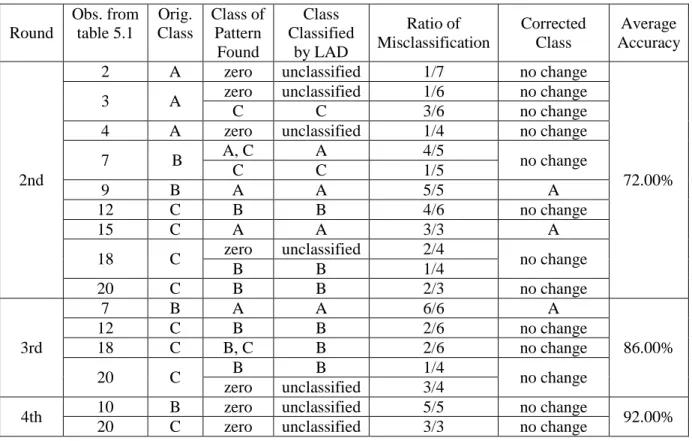
Table 5.9: Results of LAD analysis with RCA of the AHP dataset ... 32

Table 5.10: Results of LAD analysis with RCA of the VRS dataset ... 32

Table 5.11:Results of LAD analysis with RCA of the VRS dataset ... 33

Table 5.12: Results of LAD analysis with RCA of the CRS dataset ... 34

Table 5.14: RCA results of 1st round analysis of the AHP dataset ... 36

Table 5.15: Results of LAD Classification with RCA of the AHP dataset ... 37

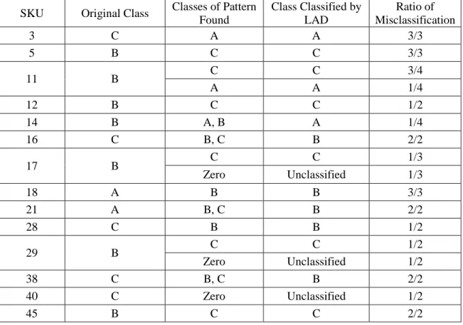
Table 5.16: Misclassified observations from 1st round analysis of the Optimal dataset ... 39

Table 5.17: RCA results of 1st round analysis of the Optimal dataset ... 40

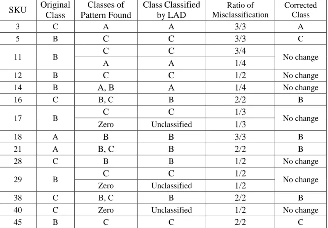
Table 5.18: Misclassification and RCA results of 2nd round analysis on Optimal dataset ... 40

Table 5.19: Misclassification and RCA results of 3rd round analysis on Optimal dataset ... 41

Table 5.20: Misclassification and RCA results of 4th round analysis on Optimal dataset ... 41

Table 5.21: Misclassification and RCA results of 5th round analysis on Optimal dataset ... 42

Table 5.22: Misclassification and RCA results of 6th round analysis on Optimal dataset ... 42

Table 5.23: Misclassification and RCA results of 7th round analysis on Optimal dataset ... 42

Table 5.24: Misclassification and RCA results of 8th round analysis on Optimal dataset ... 43

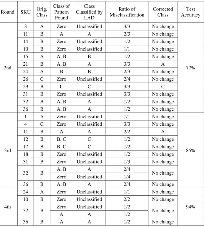
Table 5.25: Misclassified observations of 1st _{round analysis on the Scaled dataset ... 44}

Table 5.26: RCA results of the 1st round analysis on the Scaled dataset ... 45

Table 5.27: Misclassification and RCA result of 2nd round analysis on the Scaled dataset ... 45

Table 5.28: Misclassification and RCA result of 3rd round analysis on the Scaled dataset ... 46

Table 5.29: Misclassification and RCA result of 4th round analysis on the Scaled dataset ... 46

Table 6.1: Test accuracy on original and new datasets ... 50

Table 6.2: Test accuracy improvement on new datasets ... 51

Table 6.3: Test accuracy by machine learning techniques ... 52

Table 6.4: Test accuracy improvement by machine learning techniques ... 53

Table 6.5: Test accuracy on original and new datasets ... 54

Table 6.6: Test accuracy improvement on new datasets ... 54

Table 6.7: Test accuracy by machine learning technique ... 56

Table 6.9: Test accuracy on original and new datasets ... 58

Table 6.10: Paired t-Test for CRS and CRS-N ... 58

Table 6.11: Paired t-Test for VRS and VRS-N ... 59

Table 6.12: Paired t-Test for AHP and AHP-N ... 59

Table 6.13: Test accuracy on original and new datasets ... 60

Table 6.14: Paired t-Test for Scaled and Scaled-N ... 60

Table 6.15: Paired t-Test for Optimal and Optimal-N ... 61

Table 6.16: Paired t-Test for AHP and AHP-N ... 61

Table 6.17: Test accuracy of machine learning techniques on original datasets (1st inventory) .. 64

Table 6.18: Test accuracy of machine learning techniques on new datasets (1st inventory) ... 64

Table 6.19: Test accuracy of machine learning techniques on original datasets (2nd inventory) 65 Table 6.20: Test accuracy of machine learning techniques on new datasets (2nd inventory) ... 65

LIST OF FIGURES

Figure 4.1: Root cause analysis procedure for inconsistency detection ... 23

Figure 5.1: Visualisation of observations on the AHP dataset ... 31

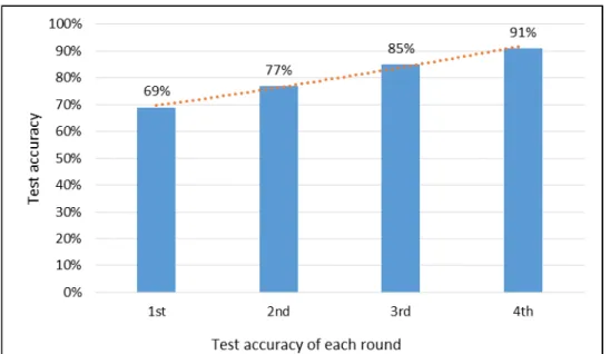
Figure 5.2: The change of test accuracy on the AHP dataset ... 38

Figure 5.3: The change of test accuracy on the Optimal dataset ... 43

Figure 5.4: The change of test accuracy on the Scaled dataset ... 46

Figure 6.1: Comparison of test accuracy between original datasets and new datasets ... 51

Figure 6.2: Comparison on test accuracy improvement of machine learning techniques ... 53

Figure 6.3: Comparison of test accuracy between original datasets and new datasets ... 55

Figure 6.4: Comparison of test accuracy improvement of machine learning techniques ... 56

LIST OF SYMBOLS AND ABBREVIATIONS

AHP Analytic Hierarchy Process

ANNs Artificial Neural Networks

BPNs backpropagation networks

CRS Constant Return to Scale

DEA Data Envelopment Analysis

DMU Decision Making Unit

FCM Fuzzy C-means

IDEA Imprecise DEA

KNN k-Nearest Neighbours

LAD Logical Analysis of Data

MCIC Multi-Criteria Inventory Classification

MDA Multiple Discriminant Analysis

NA Not Applicable

NB Naïve Bayes

OEM Original Equipment Manufacturer

OVA One-Versus-All

OVO One-Versus-One

RBF Radial Basis Function

RCA Root Cause Analysis

SKUs Stock Keeping Units

SVM Support Vector Machine

CHAPTER 1

INTRODUCTION

Spare parts inventory management plays a vital role in maintaining a competitive advantage in many industries, from capital intensive companies to service networks, such as railways, airlines, telecommunication (Boylan & Syntetos, 2010; Sarmah & Moharana, 2015; Stoll, Kopf, Schneider, & Lanza, 2015) etc. The purpose of classification is to consistently classify spare parts into different classes based on the similarity of items with respect to their characteristics. Wrongly classified critical spare parts and the unavailability of those critical items would have severe consequences (Sarmah & Moharana, 2015). Spare parts inventory management involves all parties, from Original Equipment Manufacturer (OEM) to distributors and end customers. Various forms of classifications have been widely performed in spare parts inventory management, inventory forecasting or production management (van Kampen, Akkerman, & van Donk, 2012).

The classification of spare parts into priority or criticality classes is the foundation for managing a large-scale and highly diverse assortment of parts (Rezaei & Dowlatshahi, 2010). Due to the massive quantity of distinct Stock Keeping Units (SKUs), it is almost impossible to control inventory by individual item or pay the same attention to all items (Babai, Ladhari, & Lajili, 2015). It is crucial to classify inventory items into classes and employ appropriate control policies conforming to these classes. Therefore, an ABC classification and certain inventory control techniques are often applied to facilitate SKU management (Fu, Lai, Miao, & Leung, 2015).

This study will propose using the Logical Analysis of Data (LAD), a pattern based machine learning technique, for spare parts inventory classification. The details of the LAD technique will be described further in Chapter 3, Methodology.

1.1 Statement of the problem

Spare parts inventory management intends to provide the right spare parts at the right time. The key problem is how to balance the cost of holding inventory and the risk of stock shortages (Kennedy, Wayne Patterson, & Fredendall, 2002). Either to maximize the profit from inventory sales or minimize the cost of inventory, we need to understand the characteristics of the machinery itself and then carry out the classification of inventories. Research on the classification of spare

parts helps to understand the nature of machinery, but we have not yet fully interpreted its attributes (van Kampen et al., 2012).

ABC analysis is one of the most widely used techniques for classification (Rezaei & Salimi, 2015; Stoll et al., 2015). The classical ABC classification is based on Pareto's Principle (Ramanathan, 2006) . Inventory is sorted by the total annual dollar usage, which is decided by unit price multiplied by annual usage rate. Though the ABC analysis is very popular for its ease of use, it concentrates exclusively on annual dollar usage and overlooks other important factors (Yu, 2011). The focus on this single criterion has resulted in taking no notice of other criteria, such as reliability, lead time, criticality, replicability, demand volume and inventory cost, which have been considered essential factors for inventory classification (Altay Guvenir & Erel, 1998; Ng, 2007; Ramanathan, 2006; Sarmah & Moharana, 2015; Stoll et al., 2015).

Multi-criteria classification methods are mostly divided into two categories, which are mathematical models and intelligence-based machine learning techniques. Mathematical models for inventory classification include analytic hierarchy process (AHP)(Lolli, Ishizaka, & Gamberini, 2014; Shamsaddini, Vesal, & Nawaser, 2015), data envelopment analysis (DEA) (Tavassoli, Faramarzi, & Saen, 2014) and fuzzy-rule-based approach (Sarmah & Moharana, 2015). On the other hand, machine learning techniques contain fuzzy c-means (FCM) clustering (Keskin & Ozkan, 2013), genetic algorithm (GA)(Altay Guvenir & Erel, 1998), artificial neural networks (ANNs) (Fariborz Y. Partovi & Anandarajan, 2002) etc. More details on classification methods will be discussed in Chapter 2, Literature Review. Despite their popularity, these methods either rely on certain assumptions about the importance of factors, or increase the complexity by recalculating classification with new inventory items. Furthermore, inconsistency in classification has been commonly found due to experts’ biases or inaccurate recordings.

1.2 Objective

The purpose of this study is to expand the classical ABC classification method by using a multi-criteria inventory classification approach based on the machine learning technique. The Logical Analysis of Data (LAD), a pattern based classification method, is proposed for our experiment. LAD is a machine learning technique which is capable of extracting useful knowledge in the form

of interpretable patterns from a dataset. The superiority of LAD is in its patterns transparency and robustness. In addition, it does not rely on any statistical techniques.

By utilizing the advantages of LAD technique, this thesis attempts to achieve the following specific objectives:

1. Extend the traditional ABC classification with multi-criteria by LAD;

2. Investigate the potential use of LAD by detecting inconsistencies of inventory classification;

3. Provide evidence of the capability of LAD for classification by comparing other machine learning classification techniques.

1.3 Organization of the Thesis

Chapter 2 introduces the literature review on inventory classification. The methodology of LAD is found in Chapter 3. The process of data analysis is described in Chapter 4. Chapter 5 shows our experimental results that establish the capability of LAD on spare parts inventory classification, which is tested on numerical examples. The statistical analysis results are summarized in Chapter 6, including the conclusions we have drawn from our research. Chapter 7 suggests several ideas for related future work. Following these concluding chapters is the bibliography.

CHAPTER 2

LITERATURE REVIEW

For decades, there has been plenty of research on inventory control and operations management with regards to the classification of products. Although there are a few excellent general reviews of classification on spare parts inventory, each to some extent reflects the researchers’ personal research interests and expertise. Due to the complexity of machine working conditions and the breadth of research, a truly comprehensive review is probably impossible, and certainly beyond the scope of this thesis. Instead, we focus on ABC classification and its extension schemes, which constitute the major goal of the research. The following brief review presents the characteristics of classical ABC classification and mathematical model based methods in addition to the principles of the popular machine learning techniques for ABC classification.

2.1 Traditional ABC classification

The traditional ABC classification is based on Pareto’s principle, also known as the 80-20 rule, which was developed at General Electric during the 1950s (Altay Guvenir & Erel, 1998; Keskin & Ozkan, 2013). The aim of ABC analysis is to categorize inventory into three classes, namely A (very important); B (moderately important) and C (relatively unimportant) (Hatefi, Torabi, & Bagheri, 2014). Class A includes all items within the cumulative value of 70-80%, class B includes all items with the cumulative value up to 95%, and the rest of the items are class Cs(Ng, 2007). Accordingly, each class is assigned a control level and a service level that are applied to all Stock Keeping Units (SKUs) in a specific class. More details on inventory control policies can be found in Silver, Pyke, and Peterson (1998).

ABC analysis is the most popular method for inventory classification by virtue of its clarity and capability. The classification of spare parts inventory is mostly based on the managerial efficiency concern and concentrates on the most valuable items (Braglia, Grassi, & Montanari, 2004). This practice inevitably overlooks other attributes of spare parts, such as lead time and reliability, and hardly satisfies the operations’ requirements for high availability at a low cost. Some researchers have introduced second criterion criticality of spare parts, aside from annual dollar usage, to extend the ABC analysis (Duchessi, Tayi, & Levy, 1988). This approach actually involves several other parameters, such as lead time and expected failure, to determine the criticality. However, either one-dimensional or two-dimensional classification schemes have limitations on the separation of

important factors from all potential useful parameters. A number of researchers have proposed the use of multiple criteria, such as lead time, reliability and obsolescence, to extend the ABC classification. The next section provides a brief review of Multi-Criteria Inventory Classification (MCIC).

2.2 Multi-criteria inventory classification

2.2.1 Analytic hierarchy process

Although classical ABC analysis is best known for its easy implementation and simplicity, it has been criticized for solely focusing on dollar usage and overlooking other crucial factors for inventory classification. Since then, many multi-criteria classification methods have been developed. One of the more popular techniques adopted in inventory classification is the analytic hierarchy process (AHP). The AHP methodology was proposed for spare parts classification from a number of authors (Cebi, Kahraman, & Bolat, 2010;Gajpal, Ganesh, & Rajendran, 1994; F. Y. Partovi & Hopton, 1994). The AHP is a decision making tool for analyzing complex problems which involve multiple criteria. The theory of tree structured AHP technique is formulated as pairwise comparisons to facilitate the decision-support procedure, which starts by calculating the relative weight of each criterion at each layer of the hierarchy and assessing the overall evaluation of all alternatives at the base level of the hierarchy.

The AHP techniques of ABC classification have been widely used. The main difference among those AHP techniques is the adoption of diverse criteria in the evaluation process. For example, F. Y. Partovi & Burton (1993) used four attributes of spare parts, which are unit cost, procurement cost, demand range and lead time, to classify inventory. Gajpal Ganesh & Rajendran (1994) proposed a scheme with three criteria, status of availability, type of spares and lead time, to estimate the criticality of spare parts by using the AHP technique.

One of the advantages of the AHP methodology is its adaptability in combining with other advanced techniques such as Artificial Neural Networks (ANNs), fuzzy logic and Data Envelopment Analysis (DEA) (Hadi-Vencheh & Mohamadghasemi, 2011; Kabir & Hasin, 2013; Shamsaddini et al., 2015). This characteristic allows users to obtain benefits from other methods and achieve a better solution; however, the AHP technique requires personal knowledge to assign

the weight of criteria. This assumption may bring about the inconsistency of inventory classification.

2.2.2 Data envelopment analysis

Another dynamic technique is Data Envelopment Analysis (DEA), which was originally developed by Charnes, Cooper, and Rhodes (1978). The principle of the DEA is to measure the relative performance of each Decision Making Unit (DMU) with multiple inputs and outputs. Initially it was used to evaluate the efficiency of non-profit and public organizations. Since then, many researchers have extended the DEA models and have successfully applied the models to many fields, such as financial efficiency and environment performance and classification (Liu, Lu, Lu, & Lin, 2013). One of these useful applications is inventory classification.

Ramanathan (2006) developed a DEA-like model combined with weighted linear programming for inventory classification. The model transfers all criteria into scalar scores and yields optimal scores for each inventory item by using weighted linear optimization, and then classifies items into classes based on the score value of items. This method may take a very long time when encountering thousands of inventory items, which is very common in industries. Ng (2007) improved the formulation with an alternative weight linear programming to solve the time cost problem, but the step for ranking criteria completely depends on users’ expertise and experience. This situation may lead to human bias and an inconsistency in inventory classification.

Most recently, researchers have proposed hybrid methods of DEA with other techniques, such as neural networks, fuzzy AHP and discriminant analysis (Hadi-Vencheh & Mohamadghasemi, 2011; Pendharkar, 2010; Tavassoli et al., 2014). The main difference among them is the way of calculating weights of the criteria of inventory items. Torabi, Hatefi, & Saleck Pay (2012) argued that most existing DEA models can only handle quantitative criteria. They developed a modified DEA-like model that takes both quantitative and qualitative criteria into consideration. The principle of the DEA-like model is that it applies concepts from an imprecise DEA (IDEA) model to ABC inventory classification.

2.3 Machine learning classification

With the development of computer science and artificial intelligence, machine learning techniques have been widely studied in many fields. One of the more common applications in machine learning is inventory classification.

2.3.1 Artificial neural networks

Artificial Neural Networks (ANN) is one of most popular techniques in machine learning. For instance, Partovi and Anandarajan (2002) introduced an Artificial Neural Networks (ANN) technique combining backpropagation and genetic algorithms into two learning methods for inventory classification purposes. The results are compared between the two learning methods and nonlinear relations among the criteria are discovered. But the meta-heuristics approach may be too difficult for inventory managers to understand and may result in less applicability in industry practices.

Simunovic, Simunovic, & Saric (2009) presented a model of neural networks to classify inventory items. They developed feed-forward neural networks trained by backpropagation and used minimum root mean square error for evaluating the performance. The final results show that the neural networks technique has better performance compared to the AHP method. Kabir & Hasin (2013) proposed an integration model of fuzzy AHP and neural networks for multi-criteria inventory classification. They adopted fuzzy AHP method to measure the weights of criteria of inventory items and similarly applied backpropagation to train the feed-forward neural networks. The performance of the model is assessed by the minimum mean absolute percentage of error between computed and predicted values.

2.3.2 Support vector machines

The support vector machine (SVM) is a supervised learning algorithm introduced by Vapnik (1995). The SVM classification method is based on the structural risk minimization principle (Yu, 2011). SVM approaches have been established as a popular machine learning tool in classification and aggression fields. Many applications of SVMs have been studied, including faults diagnosis, text classification, image detection, etc. (Guosheng & Guohong, 2008). Su, Zhou, & Mo, (2010) proposed a new classification scheme which is based on SVM to categorize the spare parts

inventory class. They employed the risk level as the indicator of inventory class according to the attributes of spare parts, such as importance, standardization level and replicability.

A comparison work was done between artificial-intelligence (AI)-based classification techniques and traditional multiple discriminant analysis (MDA) by Yu (2011). The AI-based techniques include support vector machines (SVMs), backpropagation neural networks (BPNs), and the k-nearest neighbour (k-NN). The results show the AI-based classification techniques have superiority over MDA.

2.3.3 K-nearest neighbours

The k-Nearest-Neighbours (k-NN) is another popular non-parametric classification and pattern recognition technique. The method is simple but effective in many cases (Gongde, Hui, Bell, Yaxin, & Greer, 2003). The principle of k-NN is to assign a new instance to the same class by determining the classification of instances that is closest to the new one. Selecting the k value is essential for a k-NN technique. An improved k-NN classification algorithm is proposed by Gong & Liu (2011). They developed a model that can dynamically get the value of k.

The k-NN classifier is an instance-based learning technique that requires computing the distance and ranking all training instances at each prediction, which is computationally expensive when classifying a lot of new instances or instances with many attributes. Another limitation is that the k-NN algorithm cannot learn anything from the training process and is not robust enough for noisy data (Bramer, 2013). To overcome the disadvantages, several researchers proposed modified models integrating other techniques. For example, Kalaivani & Shunmuganathan (2014) developed a k-NN classifier using a genetic algorithm to increase the capability by choosing appropriate attributes and achieving lower computational cost. Mejdoub & Ben Amar (2013) presented a scheme of k-NN algorithm to reduce attribute space by using the hierarchical classification technique.

2.3.4 Naïve Bayes

The Naïve Bayes (NB) model is a simple probabilistic classifier that is based on Bayes’ theorem with the assumption of independence among any feature (Agarwal, Jain, & Dholay, 2015). The NB algorithm incorporates the prior probability and conditional probabilities into one formula for

estimating the probability of every possible classification (Bramer, 2013). The limitation of NB is the independence assumptions between attributes. As reviewed by Jiang, Wang, Cai, & Yan (2007), many researchers have tried to overcome the limitation. For example, Ratanamahatana & Gunopulos (2003) proposed a combining decision tree NB algorithm that can choose the most relevant attributes of the training set to improve the classification accuracy. Webb, Boughton, & Wang (2005) presented an approach to relax the attribute independence assumption by averaging all of a constrained class of classifiers (called one-dependence classifiers).

CHAPTER 3

METHODOLOGY

3.1 Introduction

In general, data mining or machine learning provides data-driven analysis methods to extract useful knowledge or patterns from datasets. Data mining or machine learning is often divided into two main categories: supervised learning (predictive) and unsupervised learning (descriptive) methods. Supervised learning is to predict outputs for unseen observations by learning a set of input-output pairs, such as classification and regression, etc. Unsupervised learning is to find human-interpretable patterns by only given inputs, such as clustering and deep learning (Murphy, 2012).

Classification is to build a model for predicting the class of unknown observations as accurately as possible by providing a set of labelled datasets, which establishes the purpose of our study. A large number of studies on classification try to solve two-class (binary) problems where a classifier is built to discriminate new observations from two classes. But in many situations, more than two classes are involved in classification problems, such as inventory classification (Hadi-Vencheh & Mohamadghasemi, 2011; Shamsaddini et al., 2015), image recognition (Foody & Mathur, 2004; Joshi, Porikli, & Papanikolopoulos, 2012), cancer classification (Rifkin et al., 2003; Rui, Anagnostopoulos, & Wunsch, 2007; Zainuddin & Ong, 2011), handwritten interpretation (F. Chang, Chou, Lin, & Chen, 2004; Ou, Murphey, & Lee, 2004; Srihari, 2000), text categorization (Lewis, Yang, Rose, & Li, 2004; Weizhu, Jun, Benyu, Zheng, & Qiang, 2007) and speech recognition (Nakamura et al., 2006; Wang, Wang, Lin, Jian, & Kuok, 2006; Yang et al., 2012).

The two most common used approaches for multiclass classification are One-Versus-All (OVA) (or One-vs-Rest) and One-Versus-One (OVO) (also called all-pairs or All-vs-All) schemes. The main idea is to decompose the multiclass problems into multiple two-class problems. Given an N-class dataset, the OVA method is used to build N different binary N-classifiers by using one of the techniques, such as LAD, SVM or NB, etc. For the ith classifier, let the positive observations be all the points in class i, and let the negative observations be all the points not in class i. Let

f

( )

The OVO method is to build N (N-1) / 2 classifiers, one classifier to distinguish each pair of classes i and j. Let fijbe the classifier where class i are positive observations and class j are negative. Please note

f

f

x

( )

f x = ∑f x

Both OVA and OVO schemes are very simple and they were invented independently by many researchers. The choice between OVA and OVO methods is largely computational. It is more important to tune proper regularization classifiers as the underlying binary classifiers than to choose between OVA and OVO. For an overview study on OVA and OVO schemes, please refer to the article by Galar, Fernandez, Barrenechea, Bustince, & Herrera (2011). A good comparison between OVA and OVO schemes can be found in the article Duan, Rajapakse, & Nguyen (2007).

In this thesis, we adopt the OVA scheme to build LAD classifiers to solve multiclass classification problems; specifically, inventory classification.

3.2 Logical analysis of data

The Logical Analysis of Data (LAD) is a relatively new technique that intends to detect structural information and extract favorable knowledge in the style of interpretable patterns from datasets (Boros et al., 2000). This pattern-based supervised learning approach was initially presented by Crama, Hammer, & Ibaraki (1988). The Peter L. Hammer team plays a vital role in theoretical and applied developments of LAD. One of their successful applications of LAD was implemented in the medical field.

Recently the LAD technique has been studied with diverse applications, such as classification, feature selection, decision support, etc. (Boros et al., 2000). The advantage of LAD has enabled this technique to achieve plenty of applications in medical diagnosis, politics, economics, etc. A good review of LAD is presented by Alexe et al. (2007). A number of applications of LAD have been presented (S. Alexe et al., 2003; Dupuis, Gamache, & Pagé, 2012; P. L. Hammer & Bonates, 2006; Lejeune & Margot, 2011). The Yacout team was the first to apply the LAD technique to solve engineering problems, where most applications are in condition-based maintenance fields (Salamanca, 2007), such as equipment useful life prediction (Ragab, Ouali, Yacout, & Osman,

2014), rogue components detection (Mortada, Carroll Iii, Yacout, & Lakis, 2012), and fault diagnosis (Mortada, Yacout, & Lakis, 2013).

The LAD algorithm combines the theories of optimization, combinatorics and Boolean functions. Patterns, the essence of LAD technique’s decision rules, are needed to define discriminant function to separate observations between positive and negative in a dataset. Several studies of multiclass LAD approaches are proposed (Avila-Herrera & Subasi, 2015; Moreira, 2000; Mortada et al., 2013). Mortada et al. (2013) presented an OVO style multiclass LAD algorithm using mixed integer linear programming (MILP) approach to pattern generation, which is inspired by Moreira (2000) and Ryoo & Jang (2009). Avila-Herrera & Subasi (2015) proposed an OVA style multiclass LAD algorithm which also uses the MILP approach for pattern generation. The OVA style multiclass LAD model is adopted in our multi-criteria inventory classification study.

The implementation of the LAD algorithm is divided into three steps: data binarization, pattern generation and theory formation, test and classification.

3.2.1 Data binarization

Before conducting an analysis, data must be binarized so that it can be readable by computers. Each observation is considered a vector of m attributes that usually are shown as the non-binary format. The binarization process is used to transform attributes into Boolean variable vectors of n binary attributes. The non-binary attributes can be sorted into two categories: nominal indicators (e.g. color and critical level) and numerical indicators (e.g. price). The binarization of such nominal attributes is accomplished in an easy way by transforming each value vs of the attribute x into a Boolean variable b(x,vs) such that we obtain the formula below.

𝑏𝑏(𝑥𝑥, 𝑣𝑣𝑠𝑠) = �1,_0, 𝑥𝑥 = 𝑣𝑣_{𝑜𝑜𝑜𝑜ℎ𝑒𝑒𝑒𝑒𝑒𝑒𝑒𝑒𝑒𝑒𝑒𝑒}𝑠𝑠

As for numerical attributes, a practical binarization technique is to arrange attributes into a value-order style. Then a “cut-point”, which is a level variable (or interval variable) to indicate the attribute belong to certain level, is introduced. It means that for each attribute x and cut-point t (or cut-points t′, t″) a Boolean variable b(x, t) (or b(x, t′, t″)) shall be introduced as the following:

𝑏𝑏(𝑥𝑥, 𝑜𝑜) = �0,_1, 𝑥𝑥 < 𝑜𝑜_{𝑥𝑥 ≥ 𝑜𝑜} or 𝑏𝑏(𝑥𝑥, 𝑜𝑜′, 𝑜𝑜″) = �1, 𝑜𝑜′ < 𝑥𝑥 < 𝑜𝑜″

0, 𝑜𝑜𝑜𝑜ℎ𝑒𝑒𝑒𝑒𝑒𝑒𝑒𝑒𝑒𝑒𝑒𝑒

The cut-point t is the average value of vn and vn-1 (vn<vn-1) such that vn marks as one (1) and vn-1 marks as zero (0) or vice versa. The interval cut-point is formed by every two cut-points.

One example binarization procedure is presented. Suppose we have a sample dataset shown in Table 3.1, where the first and third attributes are numerical, while the second one is nominal.

Table 3.1: Sample of dataset

Label Obs. x1 x2 x3 D+ 1 1038 critical 7 2 855 critical 3 3 594 important 6 D- 4 455 important 4 5 268 regular 7 6 703 important 4

First we arrange numerical attributes from small to large so that we can calculate cut-points. Interval cut-points are also formed based on cut-points. So we easily obtain level and interval variables shown in Table 3.2 and Table 3.3. Once we have level and interval variables, the attributes can be transformed to the Boolean form shown in Table 3.4. Thus, the binarization of the dataset is done.

Table 3.2: Level variables of attributes

b1 b2 b3 b4 b5 b6 b7 b8 b9

x1≥524.5 x1≥648.5 x1≥779 x2=critical x2=important x2=regular x3≥3.5 x3≥5 x3≥6.5 Table 3.3: Interval variables of attributes

b10 b11 b12 b13 b14 b15

Table 3.4: Binary of attributes Obs. b1 b2 b3 b4 b5 b6 b7 b8 b9 b10 b11 b12 b13 b14 b15 1 1 1 1 1 0 0 1 1 1 0 0 0 0 0 0 2 1 1 1 1 0 0 0 0 0 0 0 0 0 0 0 3 1 0 0 0 1 0 1 1 0 1 1 0 0 1 1 4 0 0 0 0 1 0 1 0 0 0 0 0 1 1 0 5 0 0 0 0 0 1 1 1 1 0 0 0 0 0 0 6 1 1 0 0 1 0 1 0 0 0 1 1 1 1 0

3.2.2 Pattern generation and theory formation

Patterns play a vital role in LAD algorithm due to offering straightforward interpretation of datasets. The form of the patterns is the combination of attributes to formalize rules that can define homogenous subsets in the dataset. Once attributes are binarized, a pattern can be represented as a Boolean term of a conjunction of literals:

{ } ; 1,2, , i p n i Kp P

x

Λ

Where n is the number of attributes in datasets, Kp is the set of attributes in pattern P. Xi is a binary

variable and Xi is its negation. The number of literals is called the degree of a pattern. A pure

positive (negative) pattern is defined as its attributes covering at least one positive (negative) observation but not any negative (positive) observation. One of the most common ways of pattern generation is the combinatorial enumeration technique, such as a top-down or a bottom-up approach. The top-down approach starts by regarding all uncovered observations as patterns and removes literals one by one for those patterns until achieving a prime pattern. The bottom-up approach begins with a term of degree one which covers some positive observations. If the term only covers positive observations but not any negative ones, it is a pattern. Otherwise, literals are added to the term one by one until reaching a pattern. The details of this approach can be found in the article by Boros et al. (2000). The enumerative technique to pattern generation is a time-consuming task. For terms of degree d with n Boolean variables, the number of candidate patterns

can grow to2d

( )

n

been proposed for thrifty patterns (G. Alexe et al., 2007; G. Alexe & Hammer, 2006; Boros et al., 2000; Peter L. Hammer, Kogan, Simeone, & Szedmak, 2004; Ryoo & Jang, 2009).

In our study we adopt the MILP approach to generate patterns (Avila-Herrera & Subasi, 2015; Mortada et al., 2013; Ryoo & Jang, 2009). Given an N-class binary dataset  with m observations

and n attributes, in such way we have Ci (i =1, 2, ···, N) standing for the corresponding classes. Let

Pcp be a pattern covering some observations (coverage denoted as Cov(Pcp)) from class Cp and none of observations from class Ck, (k ≠ p).

The variables involved in the pattern generation algorithm are the pattern degree d, the Boolean pattern vector y defining the composition of the pattern found, and the coverage vector w.

Constraints should be satisfied to generate a pattern Pcp for the objective function:

(1) The Boolean vector y= (y1, y2, ···, y2n) ∈｛0, 1｝2n has such elements of binarized training dataset that if yj = 1 for some j = 1,2, ···, n, then the literal xj (associated with the j-th attribute in the dataset ) is included in pattern Pcp. Similarly, if yn+j = 1 then literalxj (complementary element of xj) is included in pattern Pc_p. So, each binarized attribute y_j in the training dataset can be expressed by a literal xj _{or its complement}xj in a pattern. Because a pattern cannot include both the literal xj andxj, and the degree d of a pattern is

associated with the number of literals, we have the constraints below:

= + ≤ = = ≤ ≤

+

∑

d

d

n

y

y

y

(2) A binary vector w= (w1, w2, ···, wm) (wi∈｛0, 1｝, 1≤ i ≤ m) is defined so that its elements are associated with the coverage of pattern Pci. The elements wi of vector w are the variables to minimize in the set covering problem so that for 1≤ i ≤ m, wi equals to one if observation

oi from class Cpis not covered by pattern Pcp, otherwiseequals to zero.

(3) Build an augmented matrixΜ =



_



_

elements to one and one elements to zero. Let vector u = My. The generated pattern must be able to cover at lease one observation Oi from class Cp (o_i ∈ Cp), however it is not

required to cover all the observations in class Cp. Hence generating a pure pattern Pcp with degree d has the constraints:

+ ≥ , ∈ ; (3.3)

i i p

u

nw

d i

I

A pattern for class k should not cover any observations from class p (k≠p). So the dot product of vector

u

= ≠

≤ −1, ∈ ,k 1,, ;k p; (3.4)

i k K

u

d

i

I

The formation of the pattern can be inferred from vector y, and its coverage vector w. Therefore, a pure pattern Pcp connected with class Cp , (1 ≤ p ≤ K) is determined by solving the optimal solution of the MILP problem below (Avila-Herrera & Subasi, 2015).

(3.5) . . (3.1),(3.2),(3.3),(3.4) p i i I Minimize d w s t ∈ +

∑

A pattern P is a strong pattern if and only if there is no pattern P′ such that Cov(P′) ⊃ Cov(P). A pattern is a prime pattern if removal of any of its literals makes it a non-pattern. Avila-Herrera & Subasi (2015) proved that an optimal solution (u, y, w, d) of problem (3.5) can be formed a pattern with maximum coverage and minimum degree, which produces a strong prime pattern. The strong prime pattern Pc has the following form. _p

{

}

{

}

y

y

Pc

Λ Λ

x

x

3.2.3 Test and classification

Suppose we have an N-class dataset  = 1∪2∪…∪N for training and testing wherek is

the set of observations from class k (k = 1, 2, …,N).The corresponding multi-class LAD models are denoted as  =1∪2∪…∪N, (i∩j =φ; i,j = 1, 2, …,N and i≠j ). For each new observation

(Ο∉_), a score is calculated based on generated patterns which cover this new observation. The judgement task is solved by a discriminant function that produces a score for each class based on patterns covered that new observation. The class along with the highest score is the estimation class

for this new observation. The discriminant function for classification of new observation (Ο∉ _) is formulated as below. ∈ Ο Ο =

∆

=

_∑

Patterns

P

w

          = ≤ ≤ ∈ ∈ = 1

_∑

The class of observation Οis estimated by the highest-class value of the discriminant function

∆ Ο( )calculated. Test accuracy is evaluated by the most commonly used method of cross-validation. The testing stage is for examination of the multi-class process and inconsistency in the dataset. The process of data analysis based on the LAD test result is presented in next Chapter. Once the test accuracy reaches an acceptable level (normally above 90%), the multi-class LAD model is ready to make classification for new (unseen) observations by using the discriminant function.

CHAPTER 4

THE PROCESS OF DATA ANALYSIS

In this chapter, we introduce our data analysis process when applying the Logical Analysis of Data (LAD) machine learning technique. The process contains two steps, namely a classification analysis of LAD and Root Cause Analysis (RCA) for misclassified items. We run both steps reiteratively until all inconsistent items are corrected and an acceptable test accuracy is received.

4.1 Tools

The random partition of the training datasets and the testing datasets is done by using Matlab. The implementation of LAD analysis is done by cbmLAD software which is written in C++ Programming language at École Polytechnique de Montréal. Several articles use cbmLAD as analysis tool to implement the LAD technique (Bennane & Yacout, 2012; Mortada et al., 2012; Mortada & Yacout, 2011).

4.2 LAD classification analysis procedure

The procedure of LAD classification analysis is to explore the dataset and to detect any problems with the dataset.

1. Suppose we have an inventory dataset = A ∪ B ∪ C with three classes A, B and

C. Firstly, we split the dataset  into two disjoint datasets called training dataset





 =









The observations in dataset  are set randomly into the training dataset





2. We execute cbmLAD on the training datasets and obtain the multi-class LAD classification and the corresponding patterns. Here we use 80% of dataset as the training dataset and the rest of the dataset as the testing dataset.

3. We execute cbmLAD on the testing datasets and calculate the test accuracy. The classification procedure by LAD is repeated on different training and testing sets either twenty or ten times. The number of repetition is chosen arbitrarily to ensure more persistent test results.

The test of twenty times is adopted in the first numerical example and ten times is for the second numerical example. The training datasets and testing datasets are randomly partitioned each time. Once the twenty (for first numerical example) or ten (for second numerical example) tests are finished, an average test accuracy is obtained by averaging the twenty tests’ accuracies. Those twenty or ten tests are defined as one round of analysis.

4.3 Root cause analysis for misclassification

One of the most important advantages of LAD is the transparency, which means the generated patterns can be easily interpreted. We make use of this characteristic of LAD to investigate misclassifications. In order to understand misclassifications, we examine the attributes of observations and find out the reason for a misclassification by using a procedure called Root Cause Analysis (RCA).

RCA begins by checking for any contradictions or repetitions. Contradictions in this thesis refer to two or more observations with exactly same attributes’ values but labelled as different classes. Since the basic assumption is that the attributes are enough to discriminate observations of different classes, all contradictory observations will be eliminated. Repetitions mean two or more observations are exactly the same. Since our objective in the training phase is to find patterns and the removal of repeated observation does not affect the pattern generation, under the condition of repetition, observations are considered as only one observation and other(s) are removed from dataset. The cbmLAD software is capable of detecting any contradictions or repetitions during the training and test phase.

Secondly, we take advantage of the logical interpretation of patterns by LAD. Patterns are generated during the training stage to reveal the characteristics of each class. Each pattern illustrates its coverage and shows corresponding weight of each pattern in the same class. The weight is the ratio of the number of covered observations by that pattern and all observations in the same class. The more observations covered by the pattern, the more weight the pattern has. In other

words, the patterns refer back to attributes that can explain why the items are misclassified. Inconsistent items can be found from the analysis of patterns.

4.3.1 Working mechanism of RCA procedure

In this section, we will briefly demonstrate how the RCA is applied to identify misclassified items. More details will be explained further in the Chapter 5 of numerical examples.

We use part of the first round result of LAD classification on AHP method dataset to illustrate the RCA procedure. Table 4.1 shows a sample of misclassified observations in testing. The unit price is US dollars and lead time is measured by days. ‘Number of test’ refers to how many times of an observation is tested during the 20 or 10 tests (one round of analysis).

Table 4.1: Misclassified observations of test (sample)

Test No.

Obs.

No. Part No.

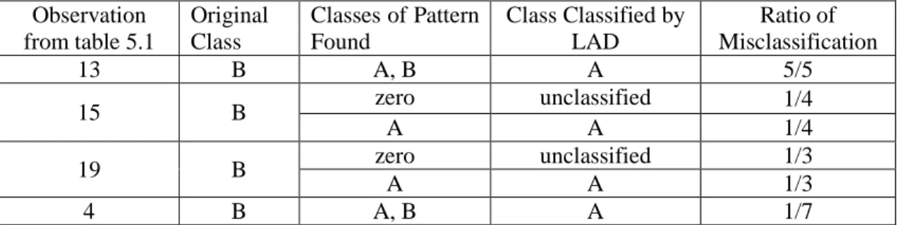
Usage Rate Unit Price Lead Time Orig. Class Classes of Patterns Found Class Classified by LAD No. of Tests 5 13 601R75 100-209 0.3 1601.58 281 B A, B A 5 10 A, B A 13 A, B A 17 A, B A 18 A, B A 9 19 601R31 7094-1 0.05 113.74 260 B zero unclassified 3 15 A A

The two misclassified items are originally from Class B. We start with No. 13 observation. The patterns, which are created during the training stage of No. 5 test, are shown in Table 4.2. The attributes of No. 13 observation are usage rate 0.3, unit price US$1,602 and lead time 281 days, which conform to both Pattern 1 of Class A and Pattern 2 of Class B. Next we examine the weight of each pattern and use the weight to decide the class of observation. Since the Pattern 1 of Class A has a larger weight (1) than Pattern 2 of Class B’s weight (0.4444), the observation is classified as Class A by LAD. Afterward, the No. 13 observation is tested 5 times over 20 tests and it is classified as Class A in all 5 tests by LAD, even though the original class is Class B. So the class of No. 13 observation changes from B to A.

No. 19 observation has the two problems of being misclassified as Class A and ‘Zero’. Here ‘Zero’ means that LAD cannot find any patterns matched for this observation or there is an equal weight

of matched patterns of different classes, which is considered as unclassified. The data from the item does not provide enough information for LAD to determine its class. The No. 19 observation has been tested 3 times over 20 tests (Test No. 7, 9 and 15, respectively) which has the outcome of 2 misclassifications and 1 correct classification. The patterns found in the No. 7 Test are shown in Table 4.3. The attributes of the No. 19 observation are usage rate 0.05, unit price US$113.74 and lead time 260 days, which match the pattern 2 of Class B. The No. 19 observation is originally labelled Class B. So it is classified correctly in the No. 7 Test.

Table 4.2: Patterns created in the No. 5 Test

Class Pattern Weight

A 1 Unit Price Greater Than 270.265 1

Lead Time Greater Than 207.5

B

1 Unit Price Less Than 270.265 0.5556 Lead Time Greater Than 139.5

2 Usage Rate Greater Than 0.065 0.4444 Lead Time Greater Than 139.5

C 1 Lead Time Less Than 139.5 1

The patterns found in the No. 9 Test are shown in Table 4.3. The attributes of No. 19 observation cannot match any patterns from Table 4.4. So the observation is considered as unclassified. The patterns found in the No. 15 Test are shown in Table 4.5. We can see that the No. 19 observation matches the pattern 1 of Class A. So it is misclassified in the No. 15 Test. Three tests receive three different results and show no consistent trend in the LAD tests, therefore, we keep this observation class unchanged.

Table 4.3: Patterns created in the No. 7 Test

Class Pattern Weight

A 1

Usage Rate Less Than 0.065

1 Unit Price Greater Than 259.92

Lead Time Greater Than 207.5

B 1

Usage Rate Greater Than 0.065

0.625 Lead Time Greater Than 125.5

2 Lead Time Greater Than 239 0.375

Table 4.4: Patterns created in the No. 9 Test

Class Pattern Weight

A 1

Usage Rate Less Than 0.065

1 Unit Price Greater Than 259.92

Lead Time Greater Than 207.5

B 1 Usage Rate Greater Than 0.065 1

Lead Time Greater Than 125.5

C 1 Lead Time Less Than 125.5 1

Table 4.5: Patterns created in the No. 15 Test

Class Pattern Weight

A

1

Usage Rate Less Than 0.065

1

Lead Time Greater Than 207.5

B 1 Usage Rate Greater Than 0.065 1

Lead Time Greater Than 125.5

C 1 Lead Time Less Than 125.5 1

By following the procedure of RCA, the explanations are found for misclassification.

1. More than one pattern matched, but the pattern weight in another class is bigger than the patterns of the original class. In other words, the item shares more common attributes with the other class than with the original class.

2. Patterns are found in only other classes. There is inconsistency in the original class.

3. No pattern is matched in the existing class. The item does not give enough information for any of the classes.

The interpretable patterns make the explanation of misclassifications straightforward and easy to understand. In order to make sure that the change of class is not arbitrary and the inconsistency is corrected, the observation class is changed when it satisfies the following situation after an RCA procedure:

1. It is always misclassified in the one different class;

2. If there is no situation 1 found and test accuracy is less than 90%, we will need a special investigation for the misclassification. (See 5.1.4).

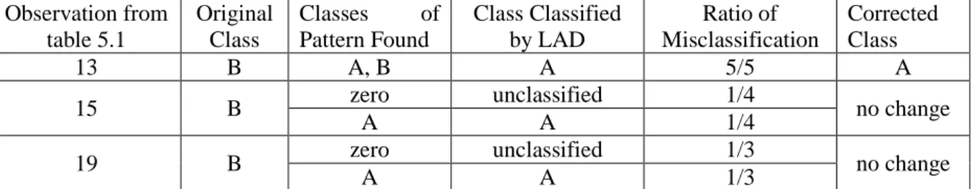
For instance, we see the No. 13 observation of Class B from Table 4.1, which is classified as Class A in all 5 tests, so the class of observation is changed from B to A. The RCA result is shown in Table 4.6.

Table 4.6: RCA result of misclassified observations

Obs. No. Usage Rate Unit Price Lead Time Orig. Class Classes of Pattern Found Class Classified by LAD No. of Tests Corrected Class 13 0.3 1601.58 281 B A, B A 5 A

19 0.05 113.74 260 B zero unclassified 3 no change

A A

After inconsistent observations are corrected, the dataset is run through another round of training and tests. Misclassified observations are checked by the RCA procedure again to detect inconsistencies. The process of LAD classification and RCA is repeated until no more inconsistent observations are found. The RCA procedure is shown in Figure 4.1.

Figure 4.1: Root cause analysis procedure for inconsistency detection

No

Yes

Yes

No

No

Yes

Start training and test Is there misclassified

End

Change class Special investigation

(see 5.1.4)

Dataset acutalisation

CHAPTER 5

LAD CLASSIFICATION: NUMERICAL EXAMPLES

In this chapter, we use two sets of numerical examples to study the LAD classification applicability, capability and its effectiveness of detecting inconsistencies by combining it with the Root Cause Analysis (RCA) procedure. First, we examine the feasibility of LAD classification on spare parts inventory and then analyze the erroneous items of classification by applying the RCA procedure. Based on the results of RCA analysis, corresponding corrections will be made. Next, both the LAD classification and the RCA procedure will be run reiteratively until all inconsistency is corrected and an acceptable test accuracy (above 90%) is received. The second numerical example study is based on medical equipment inventory. Each numerical example includes one dataset of different ABC classification methods, namely AHP, DEA, DEA-like weighted linear optimization and scaled DEA-like weighted linear optimization.

5.1 Numerical example of spare parts inventory

5.1.1 Introduction

The dataset of LAD classification on inventory is adopted from the article by Rad, Shanmugarajan, and Wahab (2011). The dataset is a set of spare parts inventory from airlines. We are able to access part of the data containing 20 observations with three results of classification methods (see Table 5.1), namely Analytic Hierarchy Process (AHP), Data Envelopment Analysis (DEA) with Constant Return to Scale (CRS) and Variable Return to Scale (VRS).

As described in Chapter 4, we classify datasets with the LAD technique and then analyze the erroneous observations of classifications by applying the procedure of Root Cause Analysis (RCA). After making corrections, both the LAD classification and the RCA procedure will be run reiteratively until all inconsistencies are corrected and an acceptable test accuracy (above 90%) is received.

The dataset contains 20 observations with five attributes: Part Number, Usage Rate, Unit Price, Lead Time and Class. The attribute Class has three results for each of the three classification methods (AHP, VRS and CRS). The attribute Part Number has no effect on the classification and is only used for the purpose of identification. To make things easier, we use the observation number as the identification of an individual inventory item.

Table 5.1: Dataset organized by three ABC classification methods

Observation Part No. Usage Rate Unit Price Lead Time ABC Classification CRS VRS AHP 1 350689-7 0.05 4.16 98 A A C 2 J221P014 0.36 8.64 30 A A C 3 AS3582-038 0.21 2.42 197 A A B 4 AS3582-232 0.36 9.28 29 A A C 5 9452K71 0.05 0.8 50 A A C 6 M39029/58-363 0.03 4.48 98 A A C 7 AS3209-014 0.13 10.72 176 B A B 8 M39029/22-191 0.05 5.6 98 B B C 9 350690-7 0.08 7.04 24 B A C 10 NSA551607ND 0.05 28.16 98 B B C 11 CC670-38730-3 0.49 706.47 188 C A B 12 3E3291-1 0.15 1152.48 148 C C B 13 601R75100-209 0.3 1601.58 281 C A B 14 AS3582-228 0.26 9.12 50 C A C 15 SL618-3CM 0.03 6.9 260 C A B 16 601R31719-5 0.05 426.79 218 C C A 17 BA670-45691-25 0.03 19.79 39 C C C 18 49001-243 0.26 93.05 103 C C C 19 601R317094-1 0.05 113.74 260 C B B 20 601R40508-35 0.08 49.75 260 C A B

For the AHP classification method, the total of 20 observations consist of 1 observation of Class A, 8 observations of Class B and 11 observations of Class C. On VRS classification method, the dataset consists of 13 observations of Class A, 3 observations of Class B and 4 observations of Class C. On CRS classification method, the dataset consists of 6 observations of Class A, 4 observations of Class B and 10 observations of Class C.

The DEA methodology was presented initially by Charnes, Cooper and Rhodes (1978). The key ingredient is efficiency, which is defined as a ratio of weighted sum of outputs to a weighted sum of inputs, where the weight structure is calculated by means of mathematical programming, and constant returns to scale (CRS) are assumed. In 1984, Banker, Charnes and Cooper developed a model with variable returns to scale (VRS). Descriptions on AHP and DEA can be found in the Chapter 2 literature review.

5.1.2 LAD Classification on dataset

We use 80% of the dataset as a training subset and 20% as a testing subset. The partitions of training and testing subsets are random. One general rule is that we keep the proportions of the three classes in those subsets the same as in the original dataset, so we can achieve a more efficient analysis of the dataset.

The process of conducting LAD classification analysis follows the instructions described in Section 4.2 ‘LAD classification analysis procedure’ in the previous chapter. After running twenty tests with randomly selecting training datasets and testing datasets, we calculate the average test accuracy. We consider these twenty tests as one round analysis of LAD classification. The confusion matrix presents the overall accuracy of the first round LAD analysis (shown in Table 5.2).

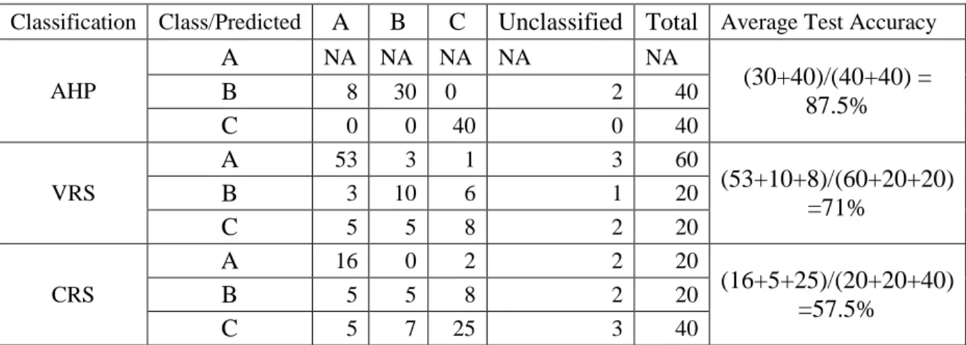
Table 5.2: The average test accuracy of the first round LAD analysis

Classification Class/Predicted A B C Unclassified Total Average Test Accuracy

AHP A NA NA NA NA NA (30+40)/(40+40) = 87.5% B 8 30 0 2 40 C 0 0 40 0 40 VRS A 53 3 1 3 60 (53+10+8)/(60+20+20) =71% B 3 10 6 1 20 C 5 5 8 2 20 CRS A 16 0 2 2 20 (16+5+25)/(20+20+40) =57.5% B 5 5 8 2 20 C 5 7 25 3 40

The numbers in Table 5.2 stand for how many observations are being tested during one round of analysis. If an observation is tested twice, it will count as 2, and so on. The ‘NA’ (Not Applicable) in Table 5.2 refers to the AHP dataset that has only one observation in Class A, so we are not able to test the Class A pattern at this time. This may be part of the reason that the LAD classification on AHP dataset reaches the best average test accuracy of 87.50%, followed by 71% for VRS dataset and 57.50% for CRS dataset. Next, we conduct the RCA procedure to detect any inconsistencies and to achieve better test accuracy (as described in section, 5.1.3.).