HAL Id: hal-00329284
https://hal.archives-ouvertes.fr/hal-00329284
Submitted on 1 Jan 2003
HAL is a multi-disciplinary open access
archive for the deposit and dissemination of
sci-entific research documents, whether they are
pub-lished or not. The documents may come from
teaching and research institutions in France or
abroad, or from public or private research centers.
L’archive ouverte pluridisciplinaire HAL, est
destinée au dépôt et à la diffusion de documents
scientifiques de niveau recherche, publiés ou non,
émanant des établissements d’enseignement et de
recherche français ou étrangers, des laboratoires
publics ou privés.
sheet
Z. Vörös, W. Baumjohann, R. Nakamura, A. Runov, T. L. Zhang, M.
Volwerk, H. U. Eichelberger, A. Balogh, T. S. Horbury, K.-H. Glaßmeier, et al.
To cite this version:
Z. Vörös, W. Baumjohann, R. Nakamura, A. Runov, T. L. Zhang, et al.. Multi-scale magnetic field
intermittence in the plasma sheet. Annales Geophysicae, European Geosciences Union, 2003, 21 (9),
pp.1955-1964. �hal-00329284�
Annales Geophysicae (2003) 21: 1955–1964 c European Geosciences Union 2003
Annales
Geophysicae
Multi-scale magnetic field intermittence in the plasma sheet
Z. V¨or¨os1, W. Baumjohann1, R. Nakamura1, A. Runov1, T. L. Zhang1, M. Volwerk1, H. U. Eichelberger1, A. Balogh2, T. S. Horbury2, K.-H. Glaßmeier3, B. Klecker4, and H. R`eme5
1Institut f¨ur Weltraumforschung der ¨OAW, Graz, Austria 2Imperial College, London, UK
3TU Braunschweig, Germany
4Max-Planck-Institut f¨ur extraterrestrische Physik, Garching, Germany 5CESR/CNRS, Toulouse, France
Received: 27 September 2002 – Revised: 14 December 2002 – Accepted: 29 January 2003
Abstract. This paper demonstrates that intermittent mag-netic field fluctuations in the plasma sheet exhibit transi-tory, localized, and multi-scale features. We propose a multifractal-based algorithm, which quantifies intermittence on the basis of the statistical distribution of the “strength of burstiness”, estimated within a sliding window. Interesting multi-scale phenomena observed by the Cluster spacecraft include large-scale motion of the current sheet and bursty bulk flow associated turbulence, interpreted as a cross-scale coupling (CSC) process.
Key words. Magnetospheric physics (magnetotail; plasma sheet) – Space plasma physics (turbulence)
1 Introduction
The study of turbulence in near-Earth cosmic plasma is im-portant in many respects. Turbulence, being in its nature a multi-scale phenomenon, may influence the transfer pro-cesses of energy, mass and momentum on both MHD and kinetic scales. Vice versa, turbulence can be driven by insta-bilities, such as magnetic reconnection or current disruption (Tetreault, 1992; Angelopoulos et al., 1999a; Klimas et al., 2000; Chang et al., 2002; Lui, 2002).
The understanding of intermittence features of fluctuations is fundamental to turbulence. Intermittence simply refers to processes which display “sporadic activity” during only a small fraction of the considered time or space. This is also the case in non-homogeneous turbulence, where the distri-bution of energy dissipation regions is sporadic and proba-bility distributions of measurable quantities are long-tailed with significant departures from Gaussianity. Rare events forming the tails of probability distribution functions, how-ever, carry a decisive amount of energy present in a process (Frisch, 1995).
Substantial experimental evidence exists for the occurence of intermittent processes within the plasma sheet.
Baumjo-Correspondence to: Z. V¨or¨os ([email protected])
hann et al. (1990) showed that within the inner plasma sheet inside of 20 RE, high-speed short-lived (∼10 s) plasma flows
are rather bursty. Angelopoulos et al. (1992) noted that those flows organize themselves into ∼10 min time scale groups called bursty bulk flows (BBF). Despite the fact that BBFs represent relatively rare events (10–20% of all mea-surements), they are the carriers of the decisive amount of mass, momentum and magnetic flux (Angelopoulos et al., 1999b; Sch¨odel et al., 2001) and can, therefore, energetically influence the near-Earth auroral regions (Nakamura et al., 2001).
So far experimental evidence for real plasma sheet tur-bulence is not unambiguous; however, its existence is sup-ported by the occurrence of plasma fluctuations in bulk flow velocity and magnetic field which are comparable or even larger than the corresponding mean values (Borovsky et al., 1997). Other characteristics of plasma sheet turbulence, such as probability distributions, mixing length, eddy viscosity, power spectra, magnetic Reynolds number, etc., were found to exhibit the expected features or to be in expected ranges predicted by turbulence theories (Borovsky et al., 1997). Though the amplitude of the velocity and magnetic field fluc-tuations increases with geomagnetic activity (Neagu et al., 2002), intense fluctuations are present independently from the level of geomagnetic activity (Borovsky et al., 1997), in-dicating that different sources or driving mechanisms might be involved in their generation. In fact, according to obser-vations by Angelopoulos et al. (1999a), at least a bi-modal state of the inner plasma sheet convection is recognizable from plasma flow magnitude probability density functions: BBF-associated intermittent jet turbulence and intermittent turbulence which occurs during non-BBF (quiet background) flows. Angelopoulos et al. (1999a) have also proposed that BBF-generated intermittent turbulence can alter transport processes in the plasma sheet and may represent a way for cross-scale coupling (CSC) to take place.
µ
(L) =1
0
L
0 L
ITER.
STEPS:
k=1
.
.
.
L/2
m
1.
µ
m
2.
µ
µ
1,1=1/4
µ
1,2=3/4
m
1.
µ
1,1m
2.
µ
1,1m
1.
µ
1,2m
2.
µ
1,2m
1=1/4
m
2=3/4
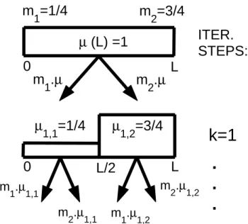
Fig. 1. Recursive construction rule for binomial distribution.
These facts call for a method which allows for analysis of both intermittence and multi-scale properties of fluctuations. In this paper we propose a multifractal technique for this pur-pose. Using both magnetic field and ion velocity data from Cluster, we will show that BBF-associated “magnetic turbu-lence” exhibits clear signatures of cross-scale energisation.
2 Multifractal approach to turbulence
In order to elucidate the basic assumptions of our approach we use a multinomial distribution model first and introduce a local parameter for quantification of the intermittence level on a given scale. Then, we discuss the range of potential scales over which the presence of cross-scale energisation might be experimentally demonstrable and mention some limitations regarding the availability of multipoint observa-tions.
2.1 Local intermittence measure (LI M)
The large-scale representation of magnetotail processes by mean values of measurable quantities is useful, but can also be misleading in characterising multi-scale phenomena when quantities observed on different scales carry physically im-portant information.
Multifractals are well suited for describing local scal-ing properties of dissipation fields in non-homogeneous tur-bulence (Frisch, 1995). Therefore, they are most suitable for a description of plasma sheet fluctuations. In non-homogeneous turbulence, the transfer of energy from large scales to smaller scales can be conveniently modeled by a multiplicative cascade process. The distribution of energy dissipation fields on small scales exhibits burstiness and in-termittence.
Let us consider a simple model example. Multinomial deterministic measures are examples of multifractals (Riedi, 1999). These consist of a simple recursive construction rule: a uniform measure µ(L) is chosen on an interval I : [0, L] and is then unevenly distributed over n > 1 (n – integer) equal subintervals of I using weights mi; i = 1, ..., n and
P
imi =1. Usually L is chosen to be 1. After the first
itera-tion we have n equal subintervals, and subinterval i contains a fraction µ(L)mi of µ(L). Next, every subinterval and the
measure on it are split in the same way recursively, having i =1, ..., nksubintervals or boxes after k iteration steps and µk,i in the box Ik,i. Figure 1 shows the simplest example of
a binomial distribution (n = 2). We note that the measure µcan be any positive and additive quantity, such as energy, mass, etc.
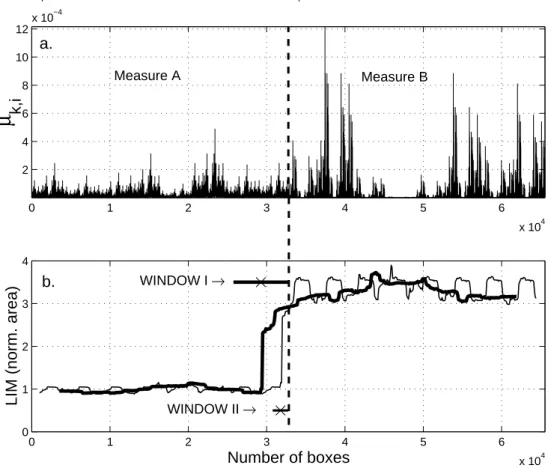
Figure 2a presents two distributions, A and B, separated by a dashed vertical line in the middle. Both mimic typical bursty “time series” like a physical variable from a turbu-lent system, however, by construction distribution A is less intermittent than distribution B. In both cases the same ini-tial mass (µ) is distributed over interval L, n = 8; k = 5 is chosen (that is nk = 32768 boxes), but the weights
mi(A) = (0.125, 0.08, 0.09, 0.16, 0.05, 0.25, 0.12, 0.125)
and mi(B) = (0.1, 0.3, 0.05, 0.002, 0.04, 0.218, 0.09, 0.2)
are different. Intermittence is larger in case B (Fig. 2a) because of the larger differences between weights (if all weights were equal, the resulting distribution would become homogeneous). Our goal is to quantify this level of inter-mittence by multifractals. The definition of multifractality in terms of the large deviation principle simply states that a dissipation field, characterized locally by a given “strength of burstiness” α, has a distribution f (α) over the considered field. It measures a deviaton of the observed α from the ex-pected value α. The corresponding (α, f (α)) large deviation spectrum is of concave shape (Riedi, 1999).
The strength of local burstiness, the so-called coarse-grain H¨older exponent α, is computed as
αi ∼
log µk,i
log[I ]k,i
, (1)
where [I ]k,i is the size of the k, i-th box and equality holds
asymptotically.
It is expected that, due to its multiplicative construction rule µk,i will decay fast as [I ]k,i →0 and k → ∞. We add
that αi <1 indicates bursts on all scales, while αi >1
char-acterizes regions where events occur sparsely (Riedi, 1999). Equation (1) then expresses the power-law dependence of the measure on resolution. Usually “histogram methods” are used for the estimation of the f (α) spectrum (also called rate function), so that the number of intervals Ik,i for which αk,i
falls in a box between αmin and αmax(the estimated
mini-mum and maximini-mum values of α) is computed and f (α) is found by regression. In this paper, however, f (α) spectra are estimated using the FRACLAB package which was devel-oped at the Institute National de Recherche en Informatique, Le Chesnay, France. Here, the well-known statistical kernel
Z. V¨or¨os et al.: Multi-scale magnetic field intermittence 1957 0 1 2 3 4 5 6 x 10⁴ 2 4 6 8 10 12x 10 −4 mi(A) ∈ [.125 .08 .09 .16 .05 .25 .12 .125] mi(B) ∈ [.1 .3 .05 .002 .04 .218 .09 .2]
µ
k,i
a.
0 1 2 3 4 5 6 x 10⁴ 0 1 2 3 4 WINDOW I →LIM (norm. area)
Number of boxes
WINDOW II →
b.
Measure A Measure B
Fig. 2. (a) Two multinomial distributions: measure A is less intermittent than measure B; dashed line in the middle separates the two measures. (b) LI M estimation for two different windows I and II.
0.5 1 1.5 2 2.5 0.2 0.3 0.4 0.5 0.6 0.7 0.8 0.9 1 α f( α ) B A
Fig. 3. Multifractal distributions for measures A and B shown in Fig. 2a.
method for density estimations is used which also yields sat-isfactory estimations for processes different from purely mul-tiplicative ones (V´ehel and Vojak, 1998; Canus et al., 1998).
A comparison of Figs. 2a and 3 indicates that the wider the f (α) spectrum is, the more intermittent the measure is. This feature was also proposed for the study of the possible role of turbulence in solar wind – magnetosphere coupling processes (V¨or¨os et al., 2002), and this feature will be used to describe magnetic field intermittence in the plasma sheet.
In order to gain appropriate information about the time evolution of intermittence from real data, we estimate f (α) within sliding overlapping windows W with a shift S W . In our model case the time axis is represented by increasing the number of subintervals Ik,i. LI M is introduced as the
to-tal area under each f (α) curve within a window W , divided by the mean area obtained from the measurements along the reference measure A. Actually, LI M(A) fluctuates around 1, due to errors introduced by finite window length. For measures exhibiting a higher level of intermittence than the reference measure A, LI M > 1. Figure 2b shows that for measures A and B, the different levels of intermittence are properly recognized by LI M. Estimations based on a larger window (Window I: W = 7000 boxes, S = 100 boxes) are more robust, but a smaller window (Window II:W = 2000 boxes, S = 100 boxes) allows for a better localization of the transition point between measures A and B (thick line in the middle of Fig. 2a).
2.2 Multi-scale LI M
Deterministic multinomial measures are self-similar in the sense that the construction rule is the same at every scale. Real data are more complex. Physical processes may have characteristic scales or may distribute energy differently over some ranges of scales. In order to study BBF-associated magnetic turbulence on both large and small scales, we in-troduce a “time scale” τ through differentiation
δBx(t, τ ) = Bx(t + τ ) − Bx(t ). (2)
Throughout the paper the GSM coordinate system is used in which the x axis is defined along the line connecting the center of the Sun to the center of the Earth. The origin is defined at the center of the Earth and is positive towards the Sun. Then, a normalized measure at a time tiis given by
µBx(ti, τ ) =
δBx2(ti, τ )
P
iδBx2(ti, τ )
. (3)
We have to mention, however, some essential limitations of this approach when a separation of spatial and temporal vari-ations is eventually addressed. A time series obtained from a single spacecraft can be used for mapping the spatial struc-ture of turbulence, using the so-called Taylor’s hypothesis, if the spatial fluctuations on a scale l pass over the spacecraft faster than they typically fluctuate in time. In the plasma sheet this is probably the case during fast BBFs (Horbury, 2000). Otherwise, Taylor’s hypothesis may not be com-pletely valid. Instead of Eq. (2) a real two-point expression, δBx+l(t ) = Bx+l(t ) − Bx(t )could be used, where l is a
dis-tance between Cluster spacecraft. The corresponding LI M, however, strongly fluctuates in a variety of cases (not shown), presumably due to mapping of physically different and struc-tured regions by individual Cluster satellites. We postpone this kind of multi-point observations to future work.
Nevertheless, Angelopoulos et al. (1999a) noticed that some characteristics of turbulence estimated from single point measurements are equivalent to ones from two-point measurements, for distances at or beyond the upper limit of the inertial range in which case Eq. (2) can be used ef-ficiently. Borovsky et al. (1997) estimated the lower limit of the inertial range to be about ion gyroperiod time scales (∼10 s in plasma sheet), over which a strong dissipation of MHD structures is expected. The upper limit of inertial range (largest scale) was identified by a plasma sheet convection time scale or by inter-substorm time scale, both of the or-der of 5 h. As known, inertial range refers to a range of wave numbers (or corresponding scales) over which turbu-lence dynamics is characterized by zero forcing and dissi-pation (Frisch, 1995). Recent theoretical and experimental work shows, however, that inertial range cascades might be exceptional. In a large variety of turbulent flows, rather bidi-rectional direct coupling (or cross scale coupling – CSC), due to nonlinearity and nonlocality between large and small scales, exists (Tsinober, 2001). While the large scales are determined by velocity fluctuations, the small scales are rep-resented by the field of velocity derivatives (vorticity, strain).
3 Data analysis
3.1 General considerations
In this paper we analyse intermittence properties of 22 Hz resolution magnetic field data from the Cluster (CL) flux-gate magnetometer (FGM) (Balogh et al., 2001) and compare those characteristics with the spin-resolution (∼4 s) velocity data from the Cluster ion spectrometry (CIS/CODIF) experi-ment (R`eme et al., 2001).
Compared with the previous model example, the estima-tion of the LI M for the BX component of the magnetic
data was somewhat different. First of all, we calculated LI M(t, τ )for different time scales τ . In the optimal case energization through a cascading process should appear on different scales that are time shifted, that is the large scales should become energized first and the small scales later. We found, however, that on various scales LI M fluctuates strongly (not shown) and using this approach it would be hard to identify an energy cascading process within an in-ertial range of scales. This was not unexpected, because cas-cade models are treated in Fourier space (wave vector space), whereas our approach represents a pure time-domain anal-ysis method (though the magnetic field data itself already contain some spatial information), so the individual scales have rather different meanings. Also, nonlinear and nonlocal direct interactions between scales may prevent experimental recognition of cascades.
Therefore, we decided to estimate LI M on several scales around 40 s, which is considered to be a typical large scale of BBF velocity fluctuations, and compute the average LI ML
(subscript L reads as large scale) from the corresponding f (α)spectra. BBF events usually last several minutes (An-gelopoulos et al., 1992), however, if τ is chosen to be several minutes long, the corresponding window length W should be even several times longer, which would make measurements of the non-stationary features of intermittence almost impos-sible.
A typical small scale was chosen experimentally. We looked for a τ (Eq. 2) which reflects the small-scale changes of the intermittence level properly. We found that fluctua-tions on time scales larger than a few seconds already exhibit similar intermittence properties as on scales around 40 s. In fact, the majority of bursty flows may remain uninteruptedly at high speed levels for a few seconds (Baumjohann et al., 1990). Therefore, we considered time scales around 0.4 s as small ones (two orders less than the chosen large scale) and the corresponding intermittence measure reads as LI MS.
This time scale may already comprise some kinetic effects. The use of 22-Hz resolution magnetic data from the FGM experiment on such small time scales implies the problem of different transfer functions for high and low frequencies. Corrections introduced by appropriate filtering had no effect on the LI M estimations.
Z. V¨or¨os et al.: Multi-scale magnetic field intermittence 1959 10:55 11 11:05 11:10 11:15 11:20 11:25 11:30 11:35 −20 0 20
Bx [nT]
CL3 :2001/08/29
10:55 11 11:05 11:10 11:15 11:20 11:25 11:30 11:35 10−20 10−10 100µ
Bx
10:55 11 11:05 11:10 11:15 11:20 11:25 11:30 11:35 10−20 10−10 100µ
Bx
10:55 11 11:05 11:10 11:15 11:20 11:25 11:30 11:35 10 15 20 25Time [UT]
LIM
L,S A B C Da.
b. (
τ
= 0.4 sec)
c. (
τ
=40 sec)
d.
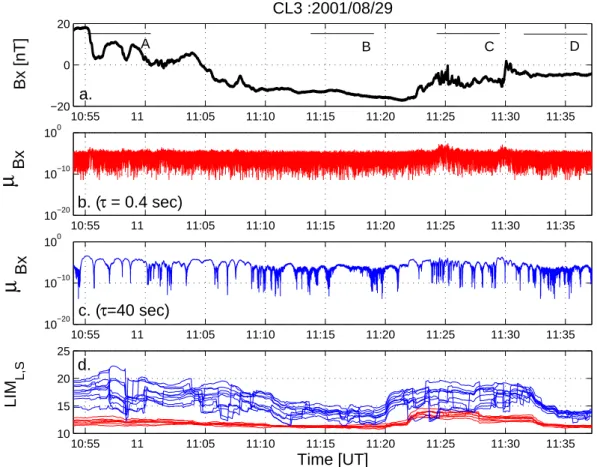
Fig. 4. (a) Magnetic field BXcomponent measured by Cluster 3; (b) the associated measure computed by using Eqs. (2) and (3) on small
scales (red colour); (c) the same on large scales (blue colour); (d) small and large scale LI ML,S.
3.2 Event overview and LI M analysis
The events we are interested in occured between 10:55 and 11:35 UT on 29 August 2001 (Fig. 4a), when CL was located at a radial distance of about 19.2 RE, near midnight. In the
following the relatively “quiet” time period from 11:15 to 11:20 UT will be used as a reference level for both LI ML
and LI MSestimations. It means that during this time period
the LI ML,Smean values equal 1.
The current sheet structure and movement during 10:55– 11:07 UT has been studied by Runov et al. (2002). Only the BX component from CL 3 will be evaluated. During the
chosen interval, CL 3 was located approximately 1500 km south of the other three spacecraft. CL traversed the neu-tral sheet from the Northern (BX ∼ 20 nT) to the Southern
Hemisphere (BX ∼ −15 nT), then BX approached BX ∼ 0
again (Fig. 4a). The correspondingly normalized small-scale (τ = 0.4 s) and large-scale (τ = 40 s) measures (Eqs. 2 and 3) are depicted by red and blue curves in Fig. 4b and c, re-spectively. In fact, Eq. (2) represents a high-pass or low-pass filter for properly chosen time shifts τ . Therefore, Fig. 4b (4c) shows an enhanced level of small-scale (large-scale) fluctuations when high-frequency (low-frequency) fluctua-tions are present in Fig. 4a. LI ML,S were computed as a
changing area under f (α) multifractal distribution curves
over the interval α ∈ (1, αmax)and within the sliding
win-dow W = 318 s. The time shift is S = 4.5 s. These parame-ters were chosen such that the opposing requirements for the stability of LI M estimations (wide window needed) and for time-localization of non-stationary events (narrow window needed) were matched. Considering the whole area under the f (α) curves, i.e. estimating LI M over α ∈ (αmin, αmax)
as in the previous section (model case), would be also possi-ble. This gives, however, the same qualitative results. During intervals of changing intermittence levels, mainly the right wing of f (α) changes. Therefore, we estimated LI M over the interval α ∈ (1, αmax). Figure 4d shows 10 red curves
of LI MS(t, τ ) computed for τ ∈ (0.3, 0.5) s, and 10 blue
curves for τ ∈ (30, 50) s. Obviously, LI MLand LI MS
ex-hibit quite different courses, and we will analyse the differ-ences in more detail.
First, we examine the f (α) multifractal spectra. Windows A, B, C and D in Fig. 4a indicate periods during which dis-tinct physical phenomena occured. The differences are evi-dent from the magnetic field BX, measures µBx and LI ML,S
evolution over time (Figs. 4a–d). We focus mainly on an in-terval between 11:23 UT and 11:33 UT, in which both LI ML
and LI MShave increased values. Period C is during this
in-terval. We contrast this interval with 10:55 to 11:10 UT, at the beginning of which a wavy flapping motion or an
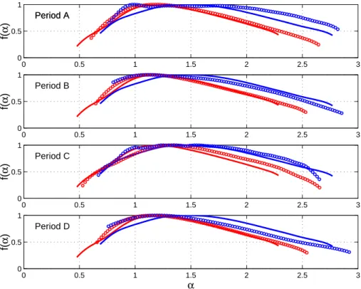
expansion-0 0.5 1 1.5 2 2.5 3 0 0.5 1 f( α ) Period APeriod A 0 0.5 1 1.5 2 2.5 3 0 0.5 1 f( α ) Period B 0 0.5 1 1.5 2 2.5 3 0 0.5 1 f( α ) Period C 0 0.5 1 1.5 2 2.5 3 0 0.5 1 α f( α ) Period D
Fig. 5. Multifractal spectra for periods A–D shown in Fig. 4a (red circles: small scales, blue circles: large scales); continuous curves with the same colour code correspond to average multifractal spectra estimated for the whole interval from 10:55 to 11:35 UT.
contraction of the current sheet is observed (Period A) with a characteristic time scale of 70–90 s (Runov et al., 2002). Periods B and C represent quiet intervals with different BX
values. The corresponding f (α) spectra are depicted by red and blue circles in Fig. 5. We also computed the global f (α) spectra for the whole BXtime series on small and large scales
from 10:55 to 11:35 UT, which are depicted by solid red and blue lines, respectively. Deviations from these average f (α) curves classify physical processes occurring during periods A–D. An examination of only the right wings of the distribu-tions leads to the following conlusions (see also Figs. 4a and d):
1. the f (α) spectra estimated on both large and small scales exceed the average f (α) only during period C; 2. during period A (large scale flapping motion), only the
large scale (blue circles) exceeds the average blue curve significantly;
3. quiet periods B and D exhibit average or narrower than average distributions.
With the definition of LI M, we have introduced a num-ber which quantifies intermittence as an area under the right wing of the f (α) distribution function. We have to empha-size, however, that f (α) distributions cannot be described or replaced by one number. The whole distribution contains more information. It is evident from Fig. 5 that the more intermittent period C is also characterized by the largest dif-ference between αmaxand αminon small scale (red circles).
Also, only in this case, the maximum of the f (α) curve is significantly shifted to the right. There are multiplicative cas-cade models for which multifractal distributions of concave shape and the underlying intermittence properties can be de-scribed by one parameter, e.g. the P-model (Halsey et al., 1986; V¨or¨os et al., 2002). However, those models cannot fit the data well because of the non-stationarity and shortness of the available time series in the plasma sheet. This is clearly visible in the case of large-scale, non-concave distributions during periods A and C (blue circles, Fig. 5). For this rea-son LI M represents a descriptor which tells more about the intermittent fluctuations than second order statistics, but less than the whole multifractal distribution function.
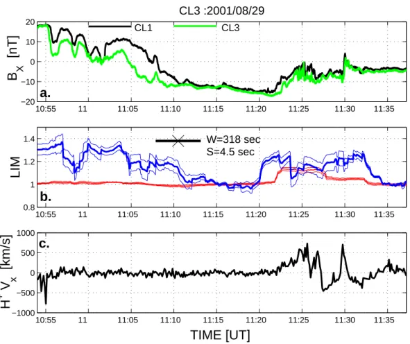
3.3 Multi-spacecraft comparison and BBF occurrence To facilitate interpretation, the BX components from two
Cluster spacecraft (CL1 and CL3) are depicted in Fig. 6a. The difference between the BXcomponents measured at the
locations of CL1 and 3 changes substantially during the con-sidered interval, indicating spatial gradients of the order of the distance between CLs within current sheet. The largest spatial gradients occur during and after the flapping motion from 10:55 to 11:10 UT. Large gradients are also present during the interval 11:22–11:30 UT. These two intervals are separated by a ∼10 min interval, from 11:10 to 11:21 UT, characterized by small spatial gradients and −18 < BX <
−10 nT. Therefore, the spacecraft are outside of the cur-rent sheet. There are two more periods when the observed
Z. V¨or¨os et al.: Multi-scale magnetic field intermittence 1961 10:55 11 11:05 11:10 11:15 11:20 11:25 11:30 11:35 −20 −10 0 10 20
B
X[nT]
CL3 :2001/08/29
10:55 11 11:05 11:10 11:15 11:20 11:25 11:30 11:35 0.8 1 1.2 1.4LIM
W=318 sec S=4.5 sec 10:55 11 11:05 11:10 11:15 11:20 11:25 11:30 11:35 −1000 −500 0 500 1000TIME [UT]
H
+V
x[km/s]
a.
b.
c.
CL1 CL3Fig. 6. (a) Magnetic field BXcomponents measured by Cluster 1, 3 spacecraft; (b) LI ML,Sfor small scales (red line) and large scales (blue
line), thin curves show standard deviations; (c) proton velocity data.
spatial gradients are small. The first is before 10:55 UT (BX > 18:nT), when the spacecraft were in the northern
lobe. The interval after 11:30 UT also contains small spa-tial gradients, but the BX components change from −6 to
2 nT, indicating that the spacecraft are closer to the center of current sheet.
Figure 6b shows LI ML,S(red and blue curves). Standard
deviations computed from a number of f (α) distributions (Fig. 4d) estimated around τ = 40 and 0.4 s are also de-picted by thin lines around LI ML,S(t )in Fig. 6b. Window
parameters are also indicated.
It is visible that during the large scale motion (thoroughly analysed by Runov et al., 2002) and after, until ∼11:10 UT (Fig. 6a), LI M shows enhanced intermittence level on large scales, but not on small scales (Fig. 6b). LI ML is also
high before 10:55 UT, only because the local window W ex-tends over the period of wavy motion of the current sheet. As no enhanced intermittence level is observed during the whole interval until ∼11:10 UT on small scales, we con-clude that cross-scale energisation is not present. More pre-cisely, at least in terms of intermittent fluctuations quantified by LI M, there was no CSC mechanism present that could couple large-scale energy reservoirs at the level of the MHD flow (∼40 s) to the small scales (∼0.4 s). We cannot exclude,
however, other mechanisms of CSC not directly associated with LI M changes. LI MLtends to decrease rapidly after
11:10 UT because data from outside the current sheet influ-ence its estimation.
Between 11:20 and 11:35 UT, both LI MLand LI MS
in-crease. This enhancement is clearly associated with high frequency intermittent fluctuations in BX (Fig. 6a; see also
the global spectrum for period C in Fig. 5) and with the oc-curence of a BBF. In Fig. 6c we show the proton velocity data from CIS/CODIF experiment (H+VX; GSM). Figure 7a
shows the magnetic field BZcomponent of the magnetic field
measured by CL3, while Figs. 7b–d show BX, proton
veloc-ity and LI M at better time resolution than in Fig. 6. Four windows centered on points marked by crosses in-dicate the times when LI ML,S significantly increase or
de-crease relative to the quiet level (LI ML,S ∼1). Vertical red
and blue arrows indicate the starting points of increase and decrease of LI ML,S, respectively.
When the spacecraft enter the current sheet after 11:20 UT, LI MLincreases and window 1 shows that the enhancement
is associated with the appearance of large-scale fluctuations in BX, a small decrease in BZand gradual increase in VX,H+,
starting at 11:22:20 UT (see the vertical dashed line at the right end of window 1). Approximately two minutes later,
11:160 11:18 11:20 11:22 11:24 11:26 11:28 11:30 11:32 11:34 11:36 10 20
B
Z[nT]
2001/08/29
11:16 11:18 11:20 11:22 11:24 11:26 11:28 11:30 11:32 11:34 11:36 −20 −10 0 10B
X[nT]
11:16 11:18 11:20 11:22 11:24 11:26 11:28 11:30 11:32 11:34 11:36 0.8 1 1.2 1.4 1.6TIME [UT]
LIM
11:16 11:18 11:20 11:22 11:24 11:26 11:28 11:30 11:32 11:34 11:36 −1000 0 1000H
+V
x[km/s]
CL1 CL3 a. b. c. d.1
2
3
4
Fig. 7. (a) Magnetic field BZcomponent from Cluster 3; (b) Magnetic field BXcomponents from Cluster 1, 3; (c) proton velocity data; (d)
LI ML,S.
the center of window 2 points to the first significant enhance-ment of LI MS(red vertical arrow). LI MSachieved its
max-imum value 1.14 ± 0.02 within ∼40 s. The right end of win-dow 2 is clearly associated with:
1. magnetic field dipolarization (rapid increase in BZ to
∼8–10 nT in Fig. 7a);
2. appearance of high-frequency fluctuations in BX(CL3),
(in Fig. 7b);
3. BBF velocities larger than 400 km/s (Fig. 7c);
4. enhancements of energetic ion and electron fluxes on CL3 (not shown); all at ∼11:24:27 UT.
LI MS drops to 1.05 ± 0.02 at 11:27:45 UT (marked by
the red arrow from the center of window 3). This time, the right end of window 3 starts to leave behind the largest peaks of VX,H+, but that is not the only reason for the decrease in
LI MS. When LI MS decreases, LI ML remains at a high
level (1.24 ± 0.05), or even increases, due to the sudden jump in BXfrom −10 to +2 nT closely before 11:30 UT. It
was previously mentioned that after 11:30 UT, the spacecraft moved closer to the center of the current sheet. Therefore, we suppose that, due to the large-scale motion of the cur-rent sheet, which keeps LI MLat a high level, the spacecraft
appear to be outside of the region of BBF-associated turbu-lence. This is also supported by the simultaneous decrease in both LI MLand LI MS at approximately 11:32:30 UT, when
window 4 includes BX from the region with small
gradi-ents after 11:30 UT. Therefore, during the interval between the right ends of window 2 and 3, i.e. within a time period of ∼6 min from ∼11:24 to ∼11:30 UT, LI M analysis indi-cates BBF and dipolarization-associated CSC between MHD and small, possibly kinetic scales. An alternative to the CSC might be a simultaneous, but independent enhancement of in-termittent fluctuations on both large and small scales. As was mentioned earlier, an identification of the energy-cascading process is almost impossible using the applied method. The primary pile-up of energy associated with the increase in BBF velocity on large scales at 11:22:20 UT, however, seems to indicate that in this case, small-scale fluctuations are ener-gised by MHD scale rapid flows. Unambiguous evidence for or against BBF-related CSC requires a statistical ensemble of events to be analysed. We mention that inverse cascades during current disruption events were reported by Lui (1998). The large difference between LI ML and LI MS after
11:28 UT can be attributed to the prevailing large-scale mo-tion of the current sheet. The spacecraft moved closer to the center of the current sheet, where the multiscale LI M signs
Z. V¨or¨os et al.: Multi-scale magnetic field intermittence 1963 of CSC are already absent. This can be explained by the
tran-sitory and localized nature of CSC.
4 Conclusions
We proposed a windowed multifractal method to quantify lo-cal intermittence of magnetic field fluctuations obtained by Cluster. The main results of this paper comprise a multi-scale description of large-scale current sheet motion and of a BBF-associated cross-scale energisation process. We have shown as Cluster passes through different plasma regions, physical processes exhibit non-stationary intermittence properties on MHD and small, possibly kinetic scales. As any robust es-timation of turbulence characteristics requires processing of long time series (due to the presence of energetic but rare events), the observed transitory and non-stationary nature of fluctuations prevents us from unambiguously supporting or rejecting a model for plasma sheet turbulence.
The multifractal description of intermittent magnetic fluc-tuations is in accordance with previous knowledge that the change in fractal scaling properties can be associated with phase transition-like phenomenon and self organization in the plasma sheet (Chang, 1999; Consolini and Chang, 2001; Consolini and Lui, 2001; Milovanov et al., 2001). Our re-sults also support the idea of Angelopoulos et al. (1999a) that BBF-related intermittent turbulence may represent an effec-tive way for CSC. Propagating BBFs can modify a critical threshold for nonlinear instabilities or trigger further local-ized reconnections due to the free energy present on multiple scales. In this sense, our results suggest that BBFs may repre-sent those multiscale carriers of energy, flux and momentum, which lead to the avalanche-like spread of disturbances on medium or large scales (Klimas et al., 2000; Lui, 2002). In this respect classification of multiscale physical processes us-ing LI M, or multifractal distributions offers a way in which the role of turbulence in a variety of dynamical processes within the plasma sheet can be statistically evaluated.
Acknowledgements. The authors acknowledge the use of
FRA-CLAB package developed at the Institut National de Recherche en Informatique, France. ZV thanks A. Petrukovich for many valuable suggestions. The work by KHG was financially supported by the German Bundesministerium f¨ur Bildung und Wissenschaft and the German Zentrum f¨ur Luft- und Raumnfahrt under contract 50 OC 0103.
Topical Editor T. Pulkkinen thanks A. Klimas and another ref-eree for their help in evaluating this paper.
References
Angelopoulos, V., Baumjohann, W., Kennel, C. F., Coroniti, F. V., Kivelson, M. G., Pellat, R., Walker, R. J., L¨uhr, H., and Paschmann, G.: Bursty bulk flows in the inner central plasma sheet, J. Geophys. Res., 97, 4027–4039, 1992.
Angelopoulos, V., Mukai, T., and Kokubun, S.: Evidence for in-termittency in Earth’s plasma sheet and implications for self-organized criticality, Phys. Plasmas, 6, 4161–4168, 1999a.
Angelopoulos, V., Mozer, F. S., Lin, R. P., Mukai, T., Tsuruda, K., Lepping, R., and Baumjohann, W.: Comment on “Geotail survey of ion flow in the plasma sheet: Observations between 10 and
50 RE” by W. R. Paterson et al., J. Geophys. Res., 104, 17 521–
17 525, 1999b.
Balogh, A., Carr, C. M., Acu˜na, M. H., et al.: The Cluster magnetic field investigation: overview of in-flight performance and initial results, Ann. Geophysicae, 19, 1207–1217, 2001.
Baumjohann, W., Paschmann, G., and L¨uhr, H.: Characteristics of high-speed ion flows in the plasma sheet, J. Geophys. Res., 95, 3801–3810, 1990.
Borovsky, J. E., Elphic, R. C., Funsten, H. O., and Thomsen, M. F.: The Earth’s plasma sheet as a laboratory for flow turbulence in high-β MHD, J. Plasma Phys., 57, 1–34, 1997.
Canus, Ch., V´ehel, J. L., and Tricot, C.: Continuous large deviation multifractal spectrum: definition and estimation, Proc. Fractals 98, Malta, 1998.
Consolini, G. and Chang, T. S.: Magnetic field topology and crit-icality in geotail dynamics: relevance to substorm phenomena, Space Sci. Rev., 95, 309–321, 2001.
Consolini, G. and Lui, A. T. Y.: Symmetry breaking and nonlinear wave-wave interaction in current disruption: possible evidence for a phase transition, AGU Monograph on Magnetospheric Cur-rent Systems, 118, 395–401, 2001;
Chang, T.: Self-organized criticality, mult-fractal spectra, sporadic localized reconnections and intermittent turbulence in the mag-netotail, Phys. Plasmas, 6, 4137–4145, 1999.
Chang, T., Wu, Ch., and Angelopoulos, V.: Preferential acceleration of coherent magnetic structres and bursty bulk flows in Earth’s magnetotail, Phys. Scripta, T98, 48–51, 2002.
Frisch, U.: Turbulence, Cambridge University Press, 1995. Horbury, T. S.: Cluster II analysis of turbulence using correlation
functions, in Proc. Cluster II Workshop, ESA SP-449, 89–97, 2000.
Halsey, T. C., Jensen, M. H., Kadanoff, L. P., Procaccia, I., and Shraiman, B. I.: Fractal measures and their singularities: the characterization of strange sets, Phys. Rev. A, 33, 1141–1151, 1986.
Klimas, A. J., Valdivia, J. A., Vassiliadis, D., Baker, D. N., Hesse, M., and Takalo, J.: Self-organized criticality in the substorm phe-nomenon and its relation to localized reconnection in the magne-tospheric plasma sheet, J. Geophys. Res., 105, 18 765–18 780, 2000.
Lui, A. T. Y.: Multiscale and intermittent nature of current disrup-tion in the magnetotail, Phys. Space Plasmas, 15, 233–238, 1998. Lui, A. T. Y.: Multiscale phenomena in the near-Earth
magneto-sphere, J. Atmosph. Sol. Terr. Phys., 64, 125–143, 2002. Milovanov, A. V., Zelenyi, L. M., Zimbardo, G., and Veltri, P.:
Self-organized branching of magnetotail current systems near the per-colation threshold, J. Geophys. Res., 106, 6291–6307, 2001. Nakamura, R., Baumjohann, W., Sch¨odel, R., Brittnacher, M.,
Sergeev, V. A., Kubyshkina, M., Mukai, T., and Liou, K.: Earth-ward flow bursts, auroral streamers, and small expansions, J. Geophys. Res., 106, 10 791–10 802, 2001.
Neagu, E., Borovsky, J. E., Thomsen, M. F., Gary, S. P., Baumjo-hann, W., and Treumann, R. A.: Statistical survey of magnetic field and ion velocity fluctuations in the near-Earth plasma sheet: Active Magnetospheric Particle Trace Explorers / Ion Release Module (AMPTE/IRM) measurements, J. Geophys. Res., 107, 10.1029/2001JA000318, 2002.
R`eme, H., Aoustin, C., Bosqued, J. M., et al.: First multispacecraft ion measurements in and near the Earth’s magnetosphere with
the identical Cluster ion spectrometry (CIS) experiment, Ann. Geophysicae, 19, 1303–1354, 2001.
Riedi, R. H.: Multifractal processes, Technical Report, TR99–06, Rice University 1999.
Runov, A., Nakamura, R., Baumjohann, W., Zhang, T. L., Volwerk, M., Eichelberger, H. U., and Balogh, A.: Cluster observation of a bifurcated current sheet, Geophys. Res. Lett., in press, 2002. Sch¨odel, R., Baumjohann, W., Nakamura, R., Sergeev, V. A., and
Mukai, T.: Rapid flux transport in the central plasma sheet, J. Geophys. Res., 106, 301–313, 2001.
Tetreault, D.: Turbulent relaxation of magnetic fields 2. Self-organization and intermittency, J. Geophys. Res., 97, 8541–8547, 1992.
Tsinober, A.: An informal introduction to turbulence, Kluwer Aca-demic Publishers, 2001.
V´ehel, J. L. and Vojak, R.: Multifractal analysis of Choquet capac-ities: preliminary results, Adv. Appl. Math., 20(1), 1–43, 1998. V¨or¨os, Z., Jankoviˇcov´a, D., and Kov´acs, P.: Scaling and
singular-ity characteristics of solar wind and magnetospheric fluctuations, Nonlin. Proc. Geophys., 9, 149–162, 2002.