Quantitative Finance under rough volatility

HAL Id: tel-02372962

https://tel.archives-ouvertes.fr/tel-02372962

HAL is a multi-disciplinary open access archive for the deposit and dissemination of sci-entific research documents, whether they are pub-lished or not. The documents may come from

L’archive ouverte pluridisciplinaire HAL, est destinée au dépôt et à la diffusion de documents scientifiques de niveau recherche, publiés ou non, émanant des établissements d’enseignement et de

Omar El Euch

To cite this version:

Omar El Euch. Quantitative Finance under rough volatility. Numerical Analysis [math.NA]. Sorbonne Université, 2018. English. �NNT : 2018SORUS172�. �tel-02372962�

THÈSE

présentée pour obtenir

LE GRADE DE DOCTEUR EN SCIENCES DE

SORBONNE UNIVERSITÉS

Spécialité : Mathématiques

par

Omar

E

L

E

UCH

Quantitative Finance Under

Rough Volatility

Soutenue le 25 Septembre 2018 devant un jury composé de :

Walter

S

University of Vienna

rapporteur

Josef

T

ETH Zurich

rapporteur

Bruno

B

Université Paris-Dauphine

examinateur

Jean-Philippe

B

Capital Fund Management

examinateur

Peter

F

TU Berlin

examinateur

Jean

J

Université Pierre et Marie Curie examinateur

Gilles

P

Université Pierre et Marie Curie examinateur

Peter

T

ENSAE

examinateur

Nizar

T

Ecole Polytechnique

examinateur

Remerciements

Je tiens en premier lieu à exprimer ma plus profonde gratitude à Mathieu Rosenbaum pour son encadrement scientifique, son soutien et sa confiance. Sous sa direction, j’ai passé trois merveilleuses années pendant lesquelles j’étais totalement épanoui. Je lui suis infiniment reconnaissant!

Je remercie Walter Schachermayer et Josef Teichamnn d’avoir accepté de rapporter ma thèse. Je suis très honoré par leur lecture attentive de ce manuscrit et leur intéret pour mon travail. Je remercie également Bruno Bouchard, Jean-Philippe Bouchaud, Peter Friz, Jean Jacod, Gilles Pagès et Peter Tankov d’examiner ma thèse et de participer à ma soutenance.

Je voudrais particulièrement exprimer ma gratitude à Nizar Touzi pour m’avoir transmis la passion des mathématiques financières et encouragé à faire cette thèse. Je suis honoré d’avoir travaillé avec lui et de l’avoir au sein du jury de ma thèse.

Je remercie également mes collaborateurs Eduardo Abi Jaber, Jim Gatheral, Masaaki Fukasawa, Thibaut Mastrolia et Othmane Mounjid. Ce fut un immense plaisir de travailler avec chacun d’eux!

Toute ma reconnaissance va aussi à Marcos Costa Santos Carreira, Christa Cuchiero, Stefano De Marco, Stefan Gerhold, Julien Guyon, Blanka Horvath, Antoine Jacquier et Alexandre Richard. Les diverses discussions et interactions que j’ai eu avec chacun d’eux ont permis le bon avancement de mon travail.

Je suis reconnaissant à tous mes professeurs de l’Ecole Polytechnique et du Master "Probabilités et Finance“, en particulier Emmanuel Gobet, Nicole El Karoui et Aurélien Alfonsi pour m’avoir fait découvrir les mathématiques financières.

Un grand merci à tous les doctorants de l’Ecole Polytechnique et de Jussieu, en particulier Aditi, Eric, Hadrien, Heythem, Paul, Saad et surtout Pamela pour leur bonne humeur et pour avoir rendu mon quotidien encore plus agréable durant ces trois dernières années.

Je remercie égalemement tout le secrétariat du CMAP et du LPMA et plus particuliérement Nasséra Naar pour sa disponibilité et son aide pendant trois ans.

Pour finir, je remercie mes parents, ma soeur, mes cousines Chema et Hend, ma famille, mes amis et Mariem pour leurs encouragements et leur soutien durant cette thèse et bien avant.

Résumé

Cette thèse a pour objectif la compréhension de plusieurs aspects du caractère rugueux de la volatilité observé de manière universelle sur les actifs financiers. Ceci est fait en six étapes. Dans une première partie, on explique cette propriété à partir des comportements typiques des agents sur le marché. Plus précisément, on construit un modèle de prix microscopique basé sur les processus de Hawkes reproduisant les faits stylisés importants de la microstructure des marchés. En étudiant le comportement du prix à long terme, on montre l’émergence d’une version rugueuse du modèle de Heston (appelé modèle rough Heston) avec effet de levier. En utilisant ce lien original entre les processus de Hawkes et les modèles de Heston, on calcule dans la deuxième partie de cette thèse la fonction caractéristique du log-prix du modèle rough Heston. Cette fonction caractéristique est donnée en terme d’une solution d’une équation de Riccati dans le cas du modèle de Heston classique. On montre la validité d’une formule similaire dans le cas du modèle rough Heston, où l’équation de Riccati est remplacée par sa version fractionnaire. Cette formule nous permet de surmonter les difficultés techniques dues au caractère non markovien du modèle afin de valoriser des produits dérivés.

Dans la troisième partie, on aborde la question de la gestion des risques des produits dérivés dans le modèle rough Heston. On présente des stratégies de couverture utilisant comme instruments l’actif sous-jacent et la courbe variance forward. Ceci est fait en spécifiant la structure markovienne infini-dimensionnelle du modèle.

Étant capable de valoriser et couvrir les produits dérivés dans le modèle rough Heston, nous confrontons ce modèle à la réalité des marchés financiers dans la quatrième partie. Plus précisément, on montre qu’il reproduit le comportement de la volatilité implicite et historique. On montre également qu’il génère l’effet Zumbach qui est une asymétrie par inversion du temps observée empiriquement sur les données financières.

On étudie dans la cinquième partie le comportement limite de la volatilité implicite à la monnaie à faible maturité dans le cadre d’un modèle à volatilité stochastique général (incluant le modèle rough Bergomi), en appliquant un développement de la densité du prix de l’actif. Alors que l’approximation basée sur les processus de Hawkes a permis de traiter plusieurs questions relatives au modèle rough Heston, nous examinons dans la sixième partie une approximation markovienne s’appliquant sur une classe plus générale de modèles à volatilité rugueuse. En utilisant cette approximation dans le cas particulier du modèle rough Heston, on obtient une méthode numérique pour résoudre les équations de Riccati fractionnaires. Enfin, nous terminons cette thèse en étudiant un problème non lié à la littérature sur la volatilité rugueuse. Nous considérons le cas d’une plateforme cherchant le meilleur système de make-take fees pour attirer de la liquidité. En utilisant le cadre principal-agent, on décrit le meilleur contrat à proposer au market maker ainsi que les cotations optimales affichées par ce dernier. Nous montrons également que cette politique conduit à une meilleure liquidité et à une baisse des coûts de transaction pour les investisseurs.

The aim of this thesis is to study various aspects of the rough behavior of the volatility observed universally on financial assets. This is done in six steps.

In the first part, we investigate how rough volatility can naturally emerge from typical behav-iors of market participants. To do so, we build a microscopic price model based on Hawkes processes in which we encode the main features of the market microstructure. By studying the asymptotic behavior of the price on the long run, we obtain a rough version of the Heston model exhibiting rough volatility and leverage effect.

Using this original link between Hawkes processes and the Heston framework, we compute in the second part of the thesis the characteristic function of the log-price in the rough Heston model. In the classical Heston model, the characteristic function is expressed in terms of a solution of a Riccati equation. We show that rough Heston models enjoy a similar formula, the Riccati equation being replaced by its fractional version. This formula enables us to overcome the non-Markovian nature of the model in order to deal with derivatives pricing. In the third part, we tackle the issue of managing derivatives risks under the rough Heston model. We establish explicit hedging strategies using as instruments the underlying asset and the forward variance curve. This is done by specifying the infinite-dimensional Markovian structure of the rough Heston model.

Being able to price and hedge derivatives in the rough Heston model, we challenge the model to practice in the fourth part. More precisely, we show the excellent fit of the model to historical and implied volatilities. We also show that the model reproduces the Zumbach’s effect, that is a time reversal asymmetry which is observed empirically on financial data. While the Hawkes approximation enabled us to solve the pricing and hedging issues under the rough Heston model, this approach cannot be extended to an arbitrary rough volatility model. We study in the fifth part the behavior of the at-the-money implied volatility for small maturity under general stochastic volatility models.

In the same spirit as the Hawkes approximation, we look in the sixth part of this thesis for a tractable Markovian approximation that holds for a general class of rough volatility models. By applying this approximation on the specific case of the rough Heston model, we derive a numerical scheme for solving fractional Riccati equations.

Finally, we end this thesis by studying a problem unrelated to rough volatility. We consider an exchange looking for the best make-take fees system to attract liquidity in its platform. Using a principal-agent framework, we describe the best contract that the exchange should propose to the market maker and provide the optimal quotes displayed by the latter. We also argue that this policy leads to higher quality of liquidity and lower trading costs for investors.

Market microstructure, high frequency trading, leverage effect, rough volatility, Hawkes pro-cesses, limit theorems, Heston model, rough Heston model, fractional Brownian motion, fractional Riccati equation, forward variance curve, affine Volterra processes, stochastic Volterra equations, Markovian representation, stochastic invariance, Zumbach’s effect, Edge-worth expansion, rough volatility models, make-take fees, market making, financial regulation, principal-agent problem, stochastic control.

List of papers being part of this thesis

• O. El Euch, M. Fukasawa and M. Rosenbaum, The microstructural foundations of leverage

effect and rough volatility, Finance and Stochastics, 22(2), 241-280, 2018.

• O. El Euch and M. Rosenbaum, The characteristic function of rough Heston models, to appear in Mathematical Finance.

• O. El Euch and M. Rosenbaum, Perfect hedging in rough Heston models, to appear in Annals of Applied Probability.

• E. Abi Jaber and O. El Euch, Markovian structure of the Volterra Heston model, submitted, 2018.

• O. El Euch, J. Gatheral and M. Rosenbaum, Roughening Heston, submitted, 2018. • O. El Euch, J. Gatheral, R. Radoicic and M. Rosenbaum, The Zumbach effect under rough

Heston, submitted, 2018.

• O. El Euch, M. Fukasawa, J. Gatheral and M.Rosenbaum, Short-term at-the-money

asymptotics under stochastic volatility models, submitted, 2017.

• E. Abi Jaber and O. El Euch, Multi-factor approximations of rough volatility models, submitted, 2018.

• O. El Euch, T. Mastrolia, M. Rosenbaum and N. Touzi, Optimal make-take fees for market

Contents x

Introduction 1

Motivations . . . 1

Outline . . . 3

1 Part I: The microstructural foundations of leverage effect and rough volatility. 4 2 Part II: Characteristic function of rough Heston models . . . 8

3 Part III: Hedging under the rough Heston model . . . 12

4 Part IV: The rough Heston model in practice . . . 17

5 Part V: Short-term behavior of the at-the-money implied volatility under rough volatility . . . 18

6 Part VI: Markovian approximation of rough volatility models . . . 21

7 Part VII: Optimal make-take fees for market making regulation . . . 25

Part I The microstructural foundations of rough volatility 31 I Microstructural foundations of leverage effect and rough volatility 33 1 Introduction . . . 33

2 From high frequency features to leverage effect . . . 37

3 From high frequency features to rough volatility . . . 47

4 Proofs . . . 52

I.A Technical results . . . 66

I.B Fractional integrals and derivatives . . . 67

I.C Mittag-Leffler functions . . . 67

Part II Pricing under the rough Heston model 69 II Characteristic function of rough Heston models 71 1 Introduction . . . 71

2 From Hawkes processes to rough Heston models . . . 75

4 The characteristic function of rough Heston models . . . 84

5 Numerical application . . . 86

6 Proofs . . . 90

II.A Mittag-Leffler functions . . . 103

II.B Wiener-Hopf equations . . . 104

II.C Fractional differential equations . . . 104

Part III Hedging under the rough Heston model 107 III Perfect hedging in rough Heston models 109 1 Introduction . . . 109

2 Conditional laws of rough Heston models . . . 112

3 Characteristic function of generalized rough Heston models . . . 113

4 Hedging under generalized rough Heston models . . . 122

5 Proofs . . . 125

III.A Fractional calculus . . . 138

III.B Martingale property of the price in the generalized rough Heston model . . . 142

III.C Moments properties for Hawkes processes . . . 143

IV Markovian structure of the Volterra Heston model 147 1 Introduction . . . 147

2 Existence and uniqueness of the Volterra Heston model . . . 149

3 Markovian structure . . . 152

4 Application: square-root process in Banach space . . . 156

IV.A Existence results for stochastic Volterra equations . . . 159

IV.B Reminder on stochastic convolutions and resolvents . . . 160

Part IV The rough Heston model in practice 163 V Roughening Heston 165 1 Introduction . . . 165

2 The rough Heston model . . . 166

3 Pricing and hedging . . . 166

4 Calibration of the rough Heston model . . . 167

5 A poor man’s rough Heston model . . . 170

V.A Numerical solution of the fractional Riccati equation . . . 172

V.B Call option prices using Fourier techniques . . . 174

VI Zumbach’s effect in rough Heston model 175 1 Introduction . . . 175

2 Empirical estimation of the Zumbach effect . . . 176

Library . . . 181

VI.B Proof of (5) . . . 183

VI.C The Zumbach effect in terms of correlations in the stationary regime . . . 183

VI.D Variance computations . . . 184

Part V Short-term behavior of the at-the-money implied volatility under rough volatility models 187 VII Short-term at-the-money asymptotics under stochastic volatility models 189 1 Introduction . . . 189

2 Framework . . . 190

3 Asymptotic expansions . . . 193

4 Asymptotics for at-the-money skew and curvature . . . 199

5 The rough Bergomi model . . . 200

VII.A Conditional expectations of Wiener-Itô integrals . . . 205

Part VI Markovian approximation of rough volatility models 207 VIII Multi-factor approximation of rough volatility models 209 1 Introduction . . . 209

2 A definition of rough volatility models . . . 212

3 Multi-factor approximation of rough volatility models . . . 213

4 The particular case of the rough Heston model . . . 219

5 Proofs . . . 225

VIII.A Stochastic convolutions and resolvents . . . 237

VIII.B Some existence results for stochastic Volterra equations . . . 240

VIII.C Linear Volterra equation with continuous coefficients . . . 244

Part VIIOptimal make-take fees for market making regulation 249 IX Optimal make-take fees for market making regulation 251 1 Introduction . . . 251

2 The model . . . 253

3 Solving the market maker’s problem . . . 256

4 Designing the optimal contract . . . 258

5 Impact of the presence of the exchange on market quality and comparison with [AS08, GLFT13] . . . 264

IX.A Predictable representation . . . 271

IX.C Exchange Hamiltonian maximization . . . 276 IX.D On the verification argument for the exchange problem . . . 277

Introduction

The aim of this work is to study various aspects of rough volatility models such as the microstructural foundations of rough volatility, the pricing and hedging under these models and finding relevant model approximations for numerical computations. We also discuss an optimal make-take fees policy for market making regulation.

Motivations

The rough nature of the volatility is nowadays considered a universal feature of financial data. It has been first discovered in [GJR18] and then confirmed in [BLP16]. Indeed, empirical studies over a very wide range of assets of volatility time series have shown that the volatility exhibits a dynamic that is rougher than that of a Brownian motion. Moreover, including this stylized fact into financial models leads to a better fit of the volatility surface, see [BFG16, Fuk17]. The first step of this thesis is to understand how such feature can be generated by answering the following question:

Question 1. Can the rough behavior of the volatility be explained from microscopic interactions

between agents?

In order to answer this question, we build a tick by tick price model encoding the microscopic stylized facts observed in the market in the context of high frequency trading. This model is based on Hawkes processes. By studying the asymptotic behavior of our microscopic price dynamic in the long run, we obtain in the limit a rough version of the Heston model.

Since the discovery of this empirical feature, many works aim at rethinking classical stochastic volatility models in order to account for the rough behavior of the volatility. A way to do so is by replacing the classical Brownian motion by a fractional one with a small Hurst parameter around0.1. However, due to the non-Markovian nature of the fractional Brownian

motion, difficulties are encountered in practice when it comes to derivatives pricing. Under the classical Heston model, efficient numerical methods for option pricing have been developed in [AMST07, CM99, KJ05, Lew01] by using the explicit formula for the characteristic function of the asset log-price established in [Hes93]. The convergence result linking Hawkes processes to rough volatility may help us to extend this formula to the rough case and to answer the following question:

Question 2. Can we obtain a formula of the characteristic function in the rough Heston model? By answering the question above, numerical methods for option pricing can be developed. However, in practice, a pricing procedure is not enough. We should also be able to manage derivatives risks. This makes the question bellow important so that such model can be used in the industry:

Question 3. How do we hedge derivatives in the rough Heston model?

Once we are able to price and hedge derivatives in the rough Heston model, it will be natural to challenge the model to practice. By introducing the rough volatility feature into the Heston framework, we expect a better fit of the model to the historical and implied volatility. Hence, we raise the following issue:

Question 4. How does the rough Heston model behave in practice?

While the Hawkes approximation will enable us to answer the questions above, this approach is only specific to the rough Heston case and cannot be extended to an arbitrary rough volatility model. We can use a direct approach by applying small-time expansions of the density of the asset price to answer our next question:

Question 5. How does the at-the-money implied volatility of rough volatility models behave in the

short term?

In the same spirit as the Hawkes approximation, it is also natural to look for a tractable Markovian approximation that can be used to tackle derivatives pricing and hedging as well as numerical simulation of a general class of rough volatility models. This leads to the following question:

Question 6. Can we approximate a rough volatility model by a tractable Markovian one? Finally, we end the thesis with a topic unrelated to rough volatility. Indeed, we study the problem of optimal market making regulation. Nowadays, with the fragmentation of financial markets, exchanges are in competition and look for the best way to attract liquidity in their platforms. Hence, they apply a make-take fees system where they subsidize liquidity providers and tax liquidity consumers. Such system led to the emergence of a new type of market makers, such as high frequency traders, that aim at collecting fee rebates. However many studies have shown that these market makers tend to leave the market in a period of stress, see [MSLR17]. Hence, they stop being liquidity providers during a period of time the market needs the most liquidity. It is therefore natural to look for a way to avoid this kind of situation by answering the following question:

Question 7. What is the optimal make-take fees system that the exchange should apply on its

Outline

Outline

Each question presented above corresponds to a part of the thesis.

In Part I, we answer Question 1 by building a Hawkes-based microscopic price model able to reproduce the main features of market microstructure: high endogoneity of the market, no-arbitrage property, buying/selling asymmetry of liquidity and presence of metaorders. We prove in Chapter I that when the first three of these stylized facts are considered, the microscopic price behaves in the long run as a Heston stochastic volatility model exhibiting leverage effect. When we add the last property (presence of metaroders), we obtain in the limit a rough version of the Heston model exhibiting both leverage effect and rough volatility. Therefore we show that rough volatility is generated from the high endogeneity of the market together with the metaorders splitting phenomenon. Furthermore, we obtain that leverage effect can be at least partially explained from microstructural features.

We answer Question 2 in Part II by using the link between Hawkes processes and the rough Heston model of Part I. While the characteristic function of the log-price under the classical Heston model is given explicitly in terms of the solution of a Riccati equation, we show in Chapter II that this formula can be extended to the rough Heston model, the Riccati equation being replaced by a fractional one. In practice, fractional Riccati equations cannot be solved explicitely, but numerical methods such as the Adams scheme, presented in Chapter II, can be used.

In Part III, we tackle Question 3 by identifying the conditional law of the rough Heston model and studying its infinite-dimensional Markovian structure. In particular, we obtain in Chapter III explicit hedging strategies of derivatives by using as instruments the state variables of the model, namely the underlying asset and the forward variance curve. We also look for a general state space in which the forward variance curve lies in Chapter IV.

In Part IV, we treat Question 4 and examine the fit of the rough Heston model to the market. More precisely, we summarize in Chapter V the results obtained in Parts II and III and show the amazing fit of the rough Heston model to the SPX volatility surface. Then in Chapter VI, we answer a question raised by Jean Philippe Bouchaud about the ability of the model to reproduce a time reversal asymmetry observed in financial time series.

In Part V, we answer Question 5 by applying an Edgeworth small-time expansion of the asset price density under a general stochastic volatility framework. In particular, we obtain the behavior of the at-the-money implied skew and curvature for small maturity and apply these results to the particular case of the rough Bergomi model, see Chapter VII.

Answers to Question 6 can be found in Part VI where we study in Chapter VIII the conver-gence of multi-factor stochastic volatility models sequence to a general class of rough volatility models. This multi-factor approximation is naturally obtained by smoothing the fractional

kernel appearing in the dynamics of the variance process. By applying this approximation on the specific case of the rough Heston model, we derive a numerical scheme for solving fractional Riccati equations appearing in the characteristic function formula.

Finally, Question 7 is studied in Part VII. We consider a framework where one market maker quotes bid and ask prices on a platform held by an exchange who earns transaction costs from each market order. The intensity of market orders arrival is a deterministic function of the spread. In order to attract liquidity in its platform, we provide in Chapter IX the optimal contract that the exchange should propose to the market maker. This is done by using a principal-agent framework: First we compute the market maker optimal quotes for any contract proposed by the exchange. Then knowing the optimal quotes of the market maker, we compute the best contract that the exchange should choose. We finally study the effect of the optimal policy on the liquidity of the market, the profit and loss of the market maker and the exchange and the transaction costs for investors.

Let us now rapidly review the main results of this thesis.

1 Part I: The microstructural foundations of leverage effect and

rough volatility.

A very wide range of assets exhibits a rough dynamic of the volatility with the same order of magnitude for the roughness parameter around0.1in the Hölder sense. Understanding how

such a stylized fact can be generated is of course a natural question. Moreover, it will lead us to rough volatility models that we can manage in practice.

In Chapter I, we aim at understanding how microscopic features of the market at the high frequency scale can give rise in the long run to the crucial macroscopic stylized facts: leverage effect and rough volatility. More precisely, we build a tick by tick price model based on Hawkes processes. Then, we encode in this model the main features of market microstructure and study its long run behavior.

1.1 Building the microscopic model

Inspired by [BDHM13a, JR15], we model the tick by tick price as follows:

Pt= Nt+− Nt−,

whereNt= (Nt+, Nt−)is a bi-dimensional Hawkes process with intensityλt= (λ+t,λ−t)defined

by µ λ+ t λ− t ¶ = µ µ+ µ− ¶ + Z t 0 µ ϕ1(t − s) ϕ3(t − s) ϕ2(t − s) ϕ4(t − s) ¶ .µd N + s d N− s ¶ ,

where µ+ _andµ− _{are positive constants and}

φ = µ ϕ1 ϕ3 ϕ2 ϕ4 ¶ :R+→ M2(R+).

1. Part I: The microstructural foundations of leverage effect and rough volatility.

In this framework,λ+

td t corresponds to the probability of an upward jump ofP between times

t and t + d t. This probability has three components:

• µ+d t, the Poissonian part of the intensity, is the probability that the price goes up

because of some exogenous reason. • ¡

Z t

0 ϕ1(t − s)d N +

s ¢d t, is the probability of upward jump induced by past upward jumps.

• ¡ Z t

0 ϕ3(t − s)d N −

s ¢d t, is the probability of upward jump induced by past downward

jumps.

Similar analysis can be made onλ−

td t.

We now present the relevant stylized facts of market microstructure in our setting:

• Encoding the absence of statistical arbitrage: At the high-frequency scale, designing a strategy that is profitable on average is a very intricate task, see [ALR14]. We model this fact by assuming that the number of future upward jumps is on average equal to the number of downward jumps, namely

E[N+

t ] = E[Nt−].

This condition is satisfied by taking

µ+_{= µ}−_{, ϕ}

1+ ϕ3= ϕ2+ ϕ4. (1)

• Dealing with the asymmetry of liquidity between the bid and ask side of the order book: The fact that the ask side of the order book is more liquid than the bid side is a stylized fact commonly observed in the market, see [BCST12, BP09, HS06, HS81, TT12]. In the Hawkes framework, this is translated by an asymmetry in the kernel matrix φ

such that

ϕ3= βϕ2, β > 1. (2)

• The high degree of endogeneity of the market: Markets are highly endogenous. This means that most of the orders have no real economic motivation but are rather sent in reaction to past orders, see [FS15, HBB13]. Thanks to a population interpretation of Hawkes processes, we can show that the stability condition

S (Z ∞

0 φ(s)ds) = kϕ1k1+ βkϕ2k1< 1,

whereS denotes the spectral radius operator, should almost be violated in order to take into account the high endogeneity of the market. Hence, we assume that this spectral radius is smaller but close to unity. To do so, we index the Hawkes process by a

parameterT > 0meant to go to infinity. More precisely, we assume that the microscopic

pricePT is given by

P_tT= NtT,+− NtT,−, (3)

whereN_tT= (NtT,+, NtT,−)is a bi-dimensional Hawkes process indexed byT, with intensity

λT t = (λT,+t ,λT,−t ) defined by ÃλT,+ t λT,− t ! = µµT µT ¶ + Z t 0 φ T (t − s). Ã d NsT,+ d NsT,− ! ,

withµT _{a positive constant. The kernel matrixφ}T_:R

+→ M2(R+)is given by φT = aTφ = aT µ ϕ1 ϕ3 ϕ2 ϕ4 ¶ , aT∈ (0, 1),

and should satisfy

S (

Z _∞

0 φ(s)ds) = 1, aTT →∞−→

1, (4)

so that the high endogeneity of the market is obtained whenT is large enough.

1.1.1 Final microscopic model

The final microscopic model for the pricePT is given by (3). In order to encode the stylized

facts discussed above, Conditions (1), (2) and (4) shall be satisfied. These conditions impose the following specific structure of the kernel matrixφT_.

Assumption 1. We assume that

φT = aTφ = aT µ ϕ1 βϕ2 ϕ2 (β − 1)ϕ2+ ϕ1 ¶ ,

withϕ1,ϕ2:R+7→ R+ such thatkϕ1k1+ βkϕ2k1= 1, andaT∈ (0, 1)converging to unity asT goes

to infinity.

1.2 Generating leverage effect

In order to obtain a first non-degenerate limit in the long run, we use the following additional assumption on the asymptotic framework and the kernel matrix.

Assumption 2. There exist positive parametersλ,µandmsuch that T (1 − aT) → T →∞λ, µT= µ, and S (Z ∞ 0 xφ(x)dx) = m < ∞.

1. Part I: The microstructural foundations of leverage effect and rough volatility.

After a suitable scaling in time and space, we show that the microscopic price converges to a Heston dynamics exhibiting a negative correlation between price and volatility moves. Result 1. Under Assumptions 1 and 2, asT tends to infinity, the rescaled microscopic price

1 TP T t T= N_{t T}T,+− N_{t T}T,− T , t ∈ [0,1],

converges in law for the Skorokhod topology to the following Heston model:

Pt= 1 1 − (kϕ1k1− kϕ2k1) s 2 1 + β Z t 0 p XsdWs, with d Xt= λ m¡(β + 1) µ λ− Xt¢d t + 1 m s 1 + β2 1 + β p Xtd Bt, X0= 0,

where(W, B )is a correlated bi-dimensional Brownian motion with

d 〈W,B〉t= 1 − β

p2(1 + β2₎d t .

Result 1 shows that when β > 1, we obtain leverage effect generated by the asymmetry of liquidity between the bid and ask side of the order book. Note that Conditions (1) and (4) are also important to obtain a non-degenerate macroscopic price limit. To our knowledge, this result is the first in the literature relating in a non ad-hoc way the leverage effect to high frequency dynamics.

1.3 Generating rough volatility

The microscopic price above does not take into account an important stylized fact: The wide presence of metaorders in the market, see [AC01, LL13]. This property is a crucial feature of the market microstructure. It is translated in the Hawkes framework by considering a kernel matrixφT _{exhibiting a heavy tail as explained in [JR16b]. This leads us to replace Assumption}

2 by the following one.

Assumption 3. There existα ∈ (1/2,1)andC > 0such that

αxαZ ∞

x ϕ1(s) + βϕ2(s)d s →x→∞

C .

Moreover, for someλ∗_{> 0andµ > 0,}

Tα(1 − aT) → T →∞λ

∗_{> 0, T}1−α_µ

T → T →∞µ.

By incorporating the effect of metaorders into our microscopic model, we obtain that the limiting behavior of the price is different from that in Result 1.

Result 2. Letλ = αλ∗_{/¡CΓ(1−α)¢. Under Assumptions 1 and 3, asT tends to infinity, the rescaled} microscopic price s 1 − aT µTα Pt TT = s 1 − aT µTα (Nt TT,+− Nt TT,−), t ∈ [0,1],

converges in the sense of finite dimensional laws to the following rough Heston model:

Pt= 1 1 − (kϕ1k1− kϕ2k1) s 2 β + 1 Z t 0 p YsdWs,

withY the unique solution of

Yt= 1 Γ(α) Z t 0 (t − s) α−1_{λ¡(1 + β) − Y} s¢d s + 1 Γ(α) Z t 0 (t − s) α−1_λ s 1 + β2 λ∗_{µ(1 + β)} p Ysd Bs,

where(W, B )is a correlated bi-dimensional Brownian motion with

d 〈W,B〉t= 1 − β

p2(1 + β2₎d t .

Furthermore, the processYt has Hölder regularityα − 1/2 − εfor anyε > 0.

Result 2 shows that the limiting behavior of the microscopic price is still of Heston-type. However, a new fractional kernel(t − s)α−1 appears in the limiting dynamics and creates a

rough behavior of the volatility. Actually this kernel appears also in the Mandelbrot-van Ness representation of the fractional Brownian motionsWH

W_tH= 1 Γ(H + 1/2) Z 0 −∞¡(t − s) H −1 2_{− (−s)}H − 1 2¢dW_s+ 1 Γ(H + 1/2) Z t 0 (t − s) H −1 2dW_s.

Hence, the tail exponentαis linked to the Hurst parameter of the limiting model H = α − 1/2.

In particular, this shows that the rough behavior of the volatility is explained by the high degree of endogeneity of the market together with the wide presence of metaorders. Note that even more fundamental arbitrage-based foundations of rough volatility have been recently developed in [JR18].

2 Part II: Characteristic function of rough Heston models

By taking into account the main features of market microstructure, Result 2 shows that after a suitable scaling in time and space, the microscopic price (3) converges in the long run to a rough version of the Heston model. In Chapter II, we use this convergence result to obtain the characteristic function of the rough Heston model. This is done by computing the characteristic function of the microscopic price and then passing to the limit. From this characteristic function formula, efficient numerical methods can be applied in order to price derivatives, see [AMST07, CM99, KJ05, Lew01].

2. Part II: Characteristic function of rough Heston models

2.1 Link between the rough Heston model and Hawkes processes

In the spirit of Chapter I, we define the rough Heston model as a rough generalization of the celebrated Heston model, where the fractional kernel(t − s)α−1 is added in the definition of

the variance process:

d St= St p VtdWt Vt= V0+ 1 Γ(α) Z t 0 (t − s) α−1_{λ(θ −V} s)d s + 1 Γ(α) Z t 0 (t − s) α−1_νp Vsd Bs. (5)

The parametersλ,θ,V0 andνin (5) are positive and W andB are two Brownian motions

with correlationρ. These parameters play the same role as in the classical Heston model. The additional parameterα ∈ (1/2,1)governs the smoothness of the volatility sample paths. The well-definition of this model is established by showing the weak existence and uniqueness of a non-negative solutionV of the fractional stochastic differential equation appearing in (5),

see Proposition 3 in Chapter II. Moreover, we show that the processV isα − 1/2 − εHölder

continuous for anyε > 0. Using the link between Hawkes processes and the Heston framework, we aim at computing the characteristic function of the log-price

Xt= log(St/S0) = Z t 0 p VsdWs− 1 2 Z t 0 Vsd s.

We consider the microscopic price PT defined in (3). We make the following choice of the

kernel matrixφT _{so that Assumptions 1 and 3 are met.}

Assumption 4. There existsβ ≥ 0such that

aT = 1 − λT−α, φT= ϕTχ, where χ = 1 β + 1 µ1 β 1 β ¶ , ϕT= aTϕ, ϕ = fα,1,

with fα,1 the Mittag-Leffler density function defined in Section II.A of Chapter II.

Result 2 needs to be adapted so that the limiting process is the log-price Xt:

• Result 2 states that q_θ(1−a

T)

2µTα PTt converges to the martingale part of Xt, namely

Rt

0

p

VsdWs. So that the drift part of Xt appears in the limit, we consider the

fol-lowing modification of the microscopic price:

X_tT = s θλ 2µT2αPtT− θλ 2µT2αNtT,+.

• Result 2 leads to a vanishing initial variance in the long run. In order to avoid this phenomenon, we need to change the Poissonian part of the intensity µT into a time

Assumption 5. The baseline intensityµˆT is given by ˆ µT(t ) = µT+ ξµT¡ 1 1 − aT(1 − Z t 0 ϕ T (s)d s) − Z t 0 ϕ T_{(s)d s¢,}

withξ > 0andµT= µTα−1for someµ > 0.

Under these new conditions, we obtain the following result.

Result 3. Under Assumptions 4 and 5, the sequence of processes(X_tT)_{t ∈[0,1]}converges in law for the

Skorokhod topology to(Xt)t ∈[0,1]with

V0= θξ, ν =s λθ(1+β

2₎

µ(1 + β)2 , ρ =

1 − β p2(1 + β2₎.

2.2 The characteristic function of Hawkes processes

In order to compute the characteristic function of the log-priceXt, we compute the

character-istic function of X_tT and then we pass to the limit. X_tT being a linear combination of N_{t T}T,+

andN_{t T}T,−, we need to be able to compute the characteristic function of a multivariate Hawkes

process.

Let us consider now ad-dimensional Hawkes processN = (N1, ..., Nd)with intensity

λt=    λ1 t ... λd t    = µ(t ) + Z t 0 φ(t − s).dNs ,

whereµ : R+→ Rd+ is locally integrable andφ : R+→ Md(R+)has integrable components such

that

S ¡Z ∞

0 φ(s)ds¢ < 1.

We give a population interpretation of this process, as in [HO74], in which we considerd types

of individuals and for for each type, an individual can be either a migrant or the descendant of a migrant such that

• Migrants of typek ∈ {1,..,d} arrive as a non-homogenous Poisson process with rate µk(t ).

• Each migrant of typek ∈ {1,..,d}gives birth to children of type j ∈ {1,..,d}following a

non-homogenous Poisson process with rateφj ,k(t ).

• Each child of type k ∈ {1,..,d} also gives birth to other children of type j ∈ {1,..,d}

2. Part II: Characteristic function of rough Heston models

Then, fork ∈ {1,..,d},N_tk can be taken as the number up to timet of migrants and children

born with typek. Using this population interpretation, we are able to characterize the law the

Hawkes process and compute its characterisitic function. Result 4. For anya ∈ Rd

E[exp(i a.Nt)] = exp¡

Z t

0 ¡C (a, t − s) − 1¢.µ(s)ds¢,

whereC :Rd× R+→ Cd is solution of the following integral equation:

C (a, t ) = exp¡i a + Z t

0 φ

∗_{(s).(C (a, t − s) − 1)d s¢,}

withφ∗_{(s)the transpose ofφ(s).}

2.3 The characteristic function of rough Heston models

From Result 4, we are able to compute the characteristic function of X_tT LT(a, t ) = E[exp(i aXtT)], a ∈ R.

Moreover as a consequence of Result 3,LT(a, t )converges to the characteristic function of the

log price Xt

L(a, t ) = E[exp(i aXt)], a ∈ R,

as T goes large. This enables us to obtain a formula forL(a, t ). Let I1−α be the fractional

integral operator defined by

I1−αf (t ) = 1

Γ(1 − α) Z t

0 (t − s)

−α_{f (s)d s,}

andDα be the fractional derivative operator defined by

Dαf (t ) = 1 Γ(1 − α) d d t Z t 0 (t − s) −α_{f (s)d s.}

We have the following result.

Result 5. Assume thatρ ∈ (−1/p2, 1/p2]. Then, the characteristic function of the log price of the

rough Heston model is given by

L(a, t ) = exp¡ Z t 0 (θλ +V0 s−α Γ(1 − α))h(i a, t − s)d s¢,

whereh(i a, .)is the unique continuous solution of the following fractional Riccati equation

Dαh(i a, t ) =1 2(−a 2 − i a) + (i aρν − λ)h(i a, t ) +ν 2 2h 2_{(i a, t ), I}1−α_{h(i a, 0) = 0, (6)}

We call Equation (6) a fractional Riccati equation. It can be also written in a Volterra form as follows, h(i a, t ) = Z t 0 (t − s)α−1 Γ(α) ¡ 1 2(−a 2 − i a) + (i aρν − λ)h(i a, s) +ν 2 2 h 2_{(i a, s)¢d s.}

Whenα = 1, we obtain a classical Riccati equation that can be solved explicitly leading to the celebrated Heston formula of the characteristic function, see [Hes93]. Forα < 1, (6) cannot be solved explicitly. However, we can apply the Adams scheme on the Volterra form of (6) to solve it numerically, see Section 5.1 in Chapter II.

Thanks to the semi-closed formula of the characteristic function, pricing vanilla options becomes an easy task in this model. Finally note that this formula has been extended in [AJLP17], to the general class of Volterra affine models in which the fractional kernel is replaced by an arbitrary one.

3 Part III: Hedging under the rough Heston model

Thanks to Result 5, we are now able to price derivatives under the rough Heston model. However in practice, the interest of pricing is limited if it does not go along with a hedging strategy.

Remarking that the conditional law of a rough Heston model is still a rough Heston dynamic, we are able to use again the Hawkes framework to compute the conditional characteristic function of the rough Heston model in Chapter III. This leads us to identify the state variables of the model, namely the underlyingSt and the forward variance curve(E[Vs+t|Ft])s≥0. As

a result, any vanilla option can be perfectly hedged, in principle, using the underlying and the forward variance curve. In Chapter IV, we generalize this result for any Volterra Heston model and provide a general state space for the forward variance curve.

3.1 Conditional law of the rough Heston model

In order to derive a hedging strategy for a vanilla option with maturityT > 0and payoff f (ST),

we need to compute the dynamics of the process (E[f (ST)|Ft])t ∈[0,T ], that is identifying the

law of the rough Heston model (5) conditional onFt. We can show that the conditional law is

still a rough Heston dynamic such that the mean reversion levelθ becomes a time dependent one. Hence, it is convenient to extend the definition of the rough Heston model as follows:

d St= St p VtdWt Vt= V0+ 1 Γ(α) Z t 0 (t − s) α−1_λ(θ0 (s) − Vs)d s + 1 Γ(α) Z t 0 (t − s) α−1_νp Vsd Bs. (7)

The parametersλ,V0 andνare positive,α ∈ (1/2,1)andW andB are two Brownian motions

with correlationρ. The new mean reversion levelθ0_{is allowed to be time dependent satisfying}

3. Part III: Hedging under the rough Heston model

Assumption 6. θ0_{is a deterministic function, continuous onR}∗

+satisfying ∀u > 0; θ0(u) ≥ − V0 λΓ(1 − α)u−α, and ∀ε > 0 ∃Kε> 0; ∀u ∈ (0, 1]; θ0(u) ≤ Kεu− 1 2−ε_.

Note that the fractional stochastic differential equation in (7) admits a unique weak solution, see Theorem 2 in Chapter III. We have the following result.

Result 6. The law of the process(St0

t ,V t0

t )t ≥0= (St +t0,Vt +t0)t ≥0 is that of a rough Heston model

with the following dynamic:

d St0 t = S t0 t q Vt0 t dW t0 t , S t0 0 = St0 Vt0 t = Vt0+ 1 Γ(α) Z t 0 (t − u) α−1_λ(θt0_{(u) − V}t0 u )d u + 1 Γ(α) Z t 0 (t − u) α−1_νq_Vt0 u d But0, with(Wt0 t , B t0

t )t ≥0= (Wt0+t− Wt0, Bt0+t− Bt0)t ≥0 a two-dimensional Brownian motion with

corre-lationρ, independent ofFt0 and

θt0_{(u) = θ}0_(t 0+ u) + α λΓ(1 − α) Z t0 0 (t0− v + u)−1−α(Vv− Vt0)d v + (u + t0)−α λΓ(1 − α)(V0− Vt0),

which is anFt0-measurable function satisfying Assumption 6.

3.2 Extending the characteristic function formula

In order to obtain the dynamic of the process(E[f (ST)|Ft])t ∈[0,T ], we compute the conditional

characteristic function of XT = log(ST/S0). Thanks to Result 6, it is enough to extend the

characteristic function formula stated in Result 5 by using again the Hawkes framework. Result 7. Lett > 0andz ∈ C. Assume

λ − ρνℜ(z) > 0, a−(t ) < ℜ(z) < a+(t ), where a−(t ) =ν 2_{− 2ρνψ(t ) +}p_∆(t) 2ν2_{(1 − ρ}2₎ , a+(t ) = ν2_{− 2ρνψ(t ) −}p_∆(t) 2ν2_{(1 − ρ}2₎ , with ψ(t) = λ + αt−α Γ(1 − α), ∆(t) = 4ν 2_ψ(t)2 + ν4− 4ρν3ψ(t). Then we have E[(St)ℜ(z)] < ∞. Furthermore, R(z, t ) = E£exp(z log(St/S0)) ¤

is given by exp¡ Z t 0 h(z, t − s)(λθ 0 (s) + V0s −α Γ(1 − α))d s¢,

whereh(z, .)is the unique continuous solution of the following fractional Riccati equation: Dαh(z, s) =1 2(z 2 − z) + (zρν − λ)h(z, s) +ν 2 2h(z, s) 2_, s ≤ t, I1−αh(z, 0) = 0.

Note that the mean reversion levelθ0_{is linked to the forward variance curve as follows:}

λθ0

(t ) = Dα(E[V.] − V0)(t ) + λE[Vt].

So, we can write the characteristic function of the log-price as a functional of(E[Vs])s≥0.

Result 8. Lett > 0andz ∈ Csatisfying the assumptions of Result 7. Then R(z, t ) =exp¡ Z t 0 χ(z,t − s)E[Vs ]d s¢ with χ(z,t) =1 2(z 2 − z) + zρνh(z, t ) +ν 2 2 h(z, t ) 2_,

withh(z, .)the unique continuous solution of the fractional Riccati equation given in Result 7.

3.3 Hedging under the rough Heston model

We are now in position to compute the dynamic of a call price with maturityT > 0and strike K > 0under the rough Heston model

Ct= E[(ST− K )+|Ft].

Assuming thatρ ≤ 0, Result 7 shows that there existsa > 1such thatE[(St)a]is finite for any

timet ≥ 0. We are therefore able to use a Fourier inversion technique similar to [CM99] and

obtain that Ct= 1 2π Z b∈R ˆ g (−b)PTt (a + i b)db

with_{g (b) =}ˆ _{(i b−a)(i b−a+1)}e(1−a+i b)log(K ) and

P_tT(a + i b) = E[exp¡(a + ib)log(ST)¢|Ft],

the conditional characteristic function process. Using the fact that conditional onFt, the law

of(S,V )is still a rough Heston model and the characteristic function formula of Result 8, we

deduce that

P_tT(a + i b) =exp¡(a + ib)log(St) +

Z T −t

0 χ(a + ib,T − t − s)E[Vs+t|Ft

]d s¢

is a deterministic function of underlyingSt and the forward variance curve(E[Vs+t|Ft])s≥0.

Hence there exists a deterministic functionalC such that Ct= C (T − t , St, (E[Vs+t|Ft])s≥0).

3. Part III: Hedging under the rough Heston model

Result 9. The functionalC admits a derivative∂SC according to the spot priceSt and a Fréchet

derivative ∂VC according to the forward variance curve(E[Vs+t|Ft])s≥0. Furthermore, we have

that Ct= C0+ Z t 0 ∂SC (T − u,Su ,E[V.+u|Fu])d Su+ Z t 0 ∂VC (T − u,Su

,E[V.+u|Fu]).(dE[V.+u|Fu]),

wheredE[Vx|Fu]is the Itô differential at timeu of the martingaleMu= E[Vx|Fu],u ≤ x.

The importance of the last result is two-fold: It shows that we are able to hedge vanilla options in principle using the underlying and the forward variance curve and that the rough Heston model is Markovian in an infinite-dimensional space with state variables St and

(E[V_s+t|Ft])s≥0. Of course, in practice, this strategy will be discretized and one will use liquid

variance swaps. We can also hedge the forward variance curve risk by using one European option as the dynamics of the forward variance curve is produced by one Brownian noise.

3.4 The Markovian structure of the Volterra Heston model

After identifying the state variables of the rough Heston model, we investigate in Chapter IV a suitable general state space in which the forward variance curve lies. To do so, we extend the rough Heston model by replacing the fractional kernel (t − s)α−1 by an arbitrary one. This

leads to the Volterra Heston model defined below.

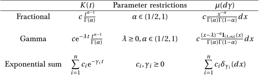
d St= St p VtdWt Vt= g0(t ) − λ Z t 0 K (t − s)Vsd s + Z t 0 K (t − s)ν p Vsd Bs. (8)

The parameters λ, V0 and ν are positive and W and B are two Brownian motions with

correlationρ. The kernel K ∈ L2_loc(R₊)is assumed to be completely monotone of the form

K (t ) =

Z ∞

0

e−xtµ(dx), t > 0,

whereµis a positive measure of locally bounded variation such that

Z _∞

0 (1 ∧ (xh)

−1/2_{)µ(dx) ≤ Ch}(γ−1)/2_, Z ∞ 0

x−1/2(1 ∧ (xh))µ(d x) ≤ C hγ/2; h > 0,

for someγ ∈ (0,2] and positive constantC. The functiong0 is assumed to be continuous and

satisfies

g0(t ) = E[Vt] + λ

Z t

0 K (t − s)E[Vs

]d s.

Hence, we can chooseg0 so that the model is consistent with the market forward variance

3.4.1 Existence and uniqueness result

We start by looking for a general condition ong0to ensure the weak existence and uniqueness

of a non-negative solution of the Volterra stochastic equation in (8) and hence the well-definition of the Volterra Heston model. LetHγ/2 be the set of locally Hölder continuous functions of any order strictly smaller thanγ/2andLbe the resolvent of the first kind ofK

defined by the unique measure of locally bounded variation such that

L ∗ K (t) = 1,

where∗is the convolution operator. We denote by∆h the following operator∆h: f 7→ f (h + ·).

We can show that∆hK ∗ L is of bounded variation and we denote byd (∆hK ∗ L)its associated

measure. Following the same approach as in [AJLP17], we obtain the following result. Result 10. Ifg0belongs to the following admissible set:

GK =©g0∈ Hγ/2; g0(0) ≥ 0and ∆hg0− (∆hK ∗ L)(0)g0− d(∆hK ∗ L) ∗ g0≥ 0,for anyh ≥ 0ª ,

there exists a unique weak non-negative solutionV of the Volterra stochastic equation (8).

Although the definition of GK seems abstract, we can show that it contains many usual

parameterizations of the forward variance curve, see Example IV.1 in Chapter IV. 3.4.2 Markovian structure

Following the same approach as in Chapter III, we identify the conditional law of the Volterra Heston model. More precisely, we obtain that the law of(St0

t ,V t0

t )t ≥0= (St +t0,Vt +t0)t ≥0 is that

of a Volterra Heston model with the following dynamics:

d St0 t = S t0 t q Vt0 t dW t0 t , S t0 0 = St0 Vt0 t = gt0(t ) − λ Z t 0 K (t − u)V t0 u d u + Z t 0 K (t − u)ν q Vt0 u d But0, with (Wt0 t , B t0

t )t ≥0 = (Wt0+t− Wt0, Bt0+t− Bt0)t ≥0 a two-dimensional Brownian motion with

correlationρ, independent ofFt0 andgt0 linked to the forward variance curve observed at

timet0, gt0(t ) = E[V t0 t |Ft0] + λ Z t 0 K (t − s)E[V t0 s |Ft0]d s.

Hence, similarly to Result 6, the Volterra Heston model is Markovian with state variables the underlyingSt andgt which is linked to the forward variance curve(E[Vs+t|Ft])s≥0. Moreover,

we are able to provide the state space in which the process(gt)t ≥0 evolves.

Result 11. GK is stochastically invariant according to(gt)t ≥0, that is

4. Part IV: The rough Heston model in practice

4 Part IV: The rough Heston model in practice

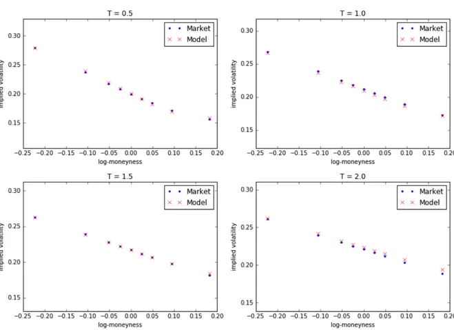
We summarize in Chapter V the results obtained under the rough Heston model and show the excellent fit of this model to the SPX volatility surface. We also study in Chapter VI the consistency of this model with a feature raised in [Zum09] concerning the time reversal asymmetry of financial time series.

4.1 Fitting the volatility surface

In Parts II and III, we build a rough version of the Heston model that appears naturally as a limit of a microscopic price and show that it enjoys tractable formulas for derivatives pricing and hedging. In Chapter V, we apply a calibration procedure on the SPX volatility surface and show the amazing fit of the model to the actual volatility surface. We also suggest, by a moments-matching procedure, an approximation method to compute instantaneously the implied volatility for a given expiry T. More precisely, we approximate the characteristic

function by the one of a classical Heston model with flat forward variance curve given by

1

T

RT

0 E[Vs]d s, correlationρand volatility of volatility parameter given by

e ν(T ) = r 3 2H + 2 ν Γ¡H +3 2 ¢ 1 T12−H .

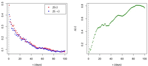
4.2 Consistency with the time reversal asymmetry

In [CB14, Zum09], it is observed empirically that the time reversal symmetry is violated in financial time series. This is the so-called Zumbach’s effect. It is done by studying the time series of daily asset log-returns (rt)t ≥0 and daily realized volatility (vt)t ≥0. More precisely,

we observe that the empirical correlation betweenr_{t −δ}2 andvt is greater that the empirical

correlation between r_t2 and v_{t −δ} for anyδ > δ0= 1day. Under the rough Heston model (7),

the daily return is given by1

rt=

Z t

t −δ0

p

VsdWs,

and the daily realized volatility is

vt=

Z t

t −δ0 Vsd s.

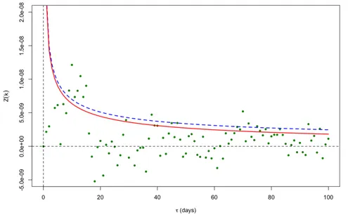
In Chapter VI, we show that the rough Heston model exhibits this phenomenon by computing

C (k, t ) = Cov(vt +kδ0, r

2

t) −Cov(r_{t +kδ}2 0, vt), t > δ0, k ∈ N.

Result 12. For smallδ0,C (k, t )is given approximatively by

C (k, t ) ∼ δ0→0 2(ρν)2δ2₀α+1g (k)E[Vt], k ∈ N, t > 0, withg (k) =_Γ(α+1)1 2 R1 0((k + s)α− (k + s − 1)α) (1 − s)αd sandα = H +1/2. In particularC (k, t ) > 0.

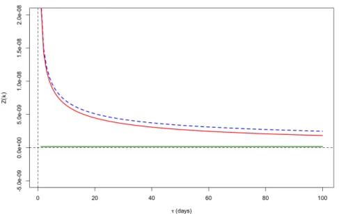
We also compute the Zumbach’s effect in the stationary regime Z (k)defined by Z (k) = lim

t →∞C or r (vt +kδ0, r

2

t) −Cor r (r_{t +kδ}2 ₀, vt).

Result 13. Consider the case where E[Vt] converges to a limiting varianceV¯∞ when t goes to

infinity. Then, for smallδ0,

Z (k) ∼ 2(ρν) 2_{p ¯V} ∞ q ν2 λ2 R_∞ 0 fα,λ(s)2d s q 2 ¯V_∞+6_λν22 R_∞ 0 fα,λ(s)2d s δ2α−1 0 g (k),

wherefα,λis the Mittag-Leffler density function,α = H+1/2andg (k) =_Γ(α+1)1 2

R1

0((k + s)α− (k + s − 1)α) (1−

s)αd s.

Note that the Zumbach’s effect is of orderδ2α−1

0 = δ 2H

0 . Hence as δ0 is small, this effect is

negligible whenH = 1/2, and this effect becomes more important when the volatility is rough,

i.e whenH is close to zero.

5 Part V: Short-term behavior of the at-the-money implied

volatility under rough volatility

While the Hawkes framework enabled us to to understand the pricing and hedging under the rough Heston model, this procedure cannot be applied for an arbitrary rough volatility model. We show in Chapter VII that asymptotic formulas for short maturity for the at-the-money skew and curvature can be obtained under a general class of stochastic volatility (that includes usual rough volatility models). This is done by applying a small-time Edgeworth expansion of the density of the asset price.

5.1 Model

We consider a general model such that the log-price is adapted to a filtrationF = (Ft)t ≥0 and

is given by d Xt= − 1 2Vtd t + p VtdWt,

where the variance processV is positive and adapted to a filtrationG = (Gt)t ≥0 smaller than

F. We assume that the Brownian motion is decomposed asWt= ρtBt+

q

1 − ρ2tB0t, with B0

independent ofGandB is aG-Brownian motion. Denoting by p(K ,θ)the put option price

with maturityθ and strikeK, we have p(F ezσ0(θ)_,θ)

Fσ0(θ) =

Z z

−∞P(Zθ≤ ζ)e

ζσ0(θ)_dζ,

where F = eX0 is the forward price,σ

0(θ) = q Rθ 0 E[Vs]d s and Z_θ= − 1 2σ0(θ)〈M〉θ+ 1 σ0(θ) M_θ, M_θ= Z θ 0 p VtdBt, 〈M〉θ= Z θ 0 Vtdt .

5. Part V: Short-term behavior of the at-the-money implied volatility under rough volatility

In order to apply a small-time expansion of the option prices, we need to make the following technical assumption that settles the asymptotic behavior of the model.

Assumption 7. There exists a family of random vectors

n

(M_θ(0), M_θ(1), M_θ(2), M_θ(3));θ ∈ (0,1)o

such that

1. the law ofM_θ(0)is standard normal for allθ > 0,

2.

sup

θ∈(0,1)kM

(i )

θ kp< ∞, i = 1, 2, 3

for allp > 0and

3. for someH ∈ (0,1/2]and² ∈ (0, H),

lim θ→0θ −2H−2² ° ° ° ° M_θ σ0(θ)− M (0) θ − θHMθ(1)− θ2HMθ(2) ° ° ° ° 1+² = 0, lim θ→0θ −H−2² ° ° ° ° 〈M〉θ σ0(θ)2− 1 − θ H_M(3) θ ° ° ° ° 1+² = 0.

Furthermore, we assume the existence of the derivatives

a(i )_θ (x) = d dx n E0[M_θ(i )|M_θ(0)= x]φ(x) o , i = 1,2,3, b_θ(x) = d 2 dx2 n E0[M_θ(1)|M_θ(0)= x]φ(x) o c_θ(x) = d 2 dx2 n E0[|M_θ(1)|2|M_θ(0)= x]φ(x) o

in the Schwartz space (i.e., the space of the rapidly decreasing smooth functions), whereφ is the standard normal density. Finally we assume that

sup θ∈(0,1) ° ° ° ° 1 θ Z θ 0 Vtdt ° ° ° °_p< ∞, _θ∈(0,1)sup ° ° ° ° ° ½ 1 θ Z θ 0 Vt(1 − ρ 2 t)dt ¾−1°_° ° ° °_p < ∞,

wherek · kp denotes theLp-norm under the probability measureP.

Note that regular stochastic volatility models satisfy Assumption 7, see Section 2.2 of Chapter VII.

5.2 Asymptotics results

Applying Assumption 7, we obtain an asymptotic expansion of the density ofZ_θ,.

Result 14. Under Assumption 7, the densityp_θ ofZ_θ satisfies

sup

x∈R

(1 + x2)α|pθ(x) − qθ(x)| = o(θ2H)

asθ → 0for anyα ∈ N, where

q_θ(x) =φ(x) − θHa(1)_θ (x) − θ2Ha(2)_θ (x) −σ0(θ) 2 (xφ(x) − θ H_a(3) θ (x)) +θ 2H 2 cθ(x) − θH_σ 0(θ) 2 bθ(x) + σ0(θ)2 8 (x 2 − 1)φ(x).

Under usual stochastic volatility models, we can in general approximateq_θ by qeθ such that

sup x∈R(1 + x 2₎α |qθ(x) −qeθ(x)| = o(θ 2H_), with e q_θ(x) =φ µ x +σ0(θ) 2 ¶ ½ 1 + κ3(θ) µ H3 µ x +σ0(θ) 2 ¶ − σ0(θ)H2 µ x +σ0(θ) 2 ¶¶ θH¾ + φ(x) µ κ4(θ)H4(x) +κ3 (θ)2 2 H6(x) ¶ θ2H_,

where κ3 andκ4 are bounded functions and Hk denotes thekth Hermite polynomial. This

enables us to compute the asymptotic behavior of the put price p(F ezσ0(θ)_,θ) for small θ,

leading to the following expansion of the implied volatility. Result 15. For anyz ∈ R,

σBS(pθz,θ) = κ2(θ) ( 1 + κ3(θ) Ã z κ2(θ)+ κ2(θ) p θ 2 ! θH +Ã 3κ 2 3(θ) 2 − κ4(θ) + (κ4(θ) − 3κ 2 3(θ)) z2 κ2 2(θ) ! θ2H ) + o(θ2H), whereκ2(θ) = σ0(θ)/ p

θ andσBS(k,θ)denotes the implied volatility with log-moneyness k and

maturityθ. This leads to the following asymptotics of the at-the-money skew and curvature

∂kσBS(0,θ) = κ3(θ)θH −1/2+ o(θ2H −1/2), ∂2 kσBS(0,θ) = 2 κ4(θ) − 3κ3(θ)2 κ2(θ) θ 2H −1 + o(θ2H −1).

6. Part VI: Markovian approximation of rough volatility models

5.3 Application to the rough Bergomi model

We apply these results to the rough Bergomi model introduced in [BFG16], where the variance process is defined as follows

Vt= E[Vt] exp ( ηH p 2H Z t 0 (t − s) H −1/2_dB s− η2 H 2 t 2H ) ,

whered 〈W,B〉t= ρd t. We can check then that Assumption 7 is satisfied and thatqeθ can be

computed explicitly with

κ3(θ) = ρηH r H 2 1 θH_σ 0(θ)3 Z θ 0 exp ( −η 2 H 8 t 2H ) Z t 0 (t − s) H −1/2_pE[V s]dsE[Vt]dt , κ4(θ) = (1 + 2ρ2)η2_HH (2H + 1)2_{(2H + 2)}+ ρ2_η2 HHβ(H + 3/2, H + 3/2) 2(H + 1/2)2 .

whereβis the beta function.

6 Part VI: Markovian approximation of rough volatility models

d St= St p VtdWt, t ∈ [0,T ], Vt= V0+ 1 Γ(H + 1/2) Z t 0 (t − s) H −1/2_λ(θ0 (s) − Vs)d s + 1 Γ(H + 1/2) Z t 0 (t − s) H −1/2_σ(V s)d Bs. (9)

The parametersλ,V0 are positive,H ∈ (0,1/2)is the Hurst parameter2,σ is a deterministic

function,θ0 _{is a mean reversion level allowed to be time dependent andW andB are two}

Brownian motions with correlation ρ. Note that the rough Heston model (7) is a particular case of (9) withσ(x) = νpx. The weak existence of such model is guaranteed by assuming

thatθ0 _{satisfies Assumption 6 and thatσis a continuous function with linear growth such that}

σ(0) = 0. In that case, the variance processV admits Hölder continuous paths of any order

strictly less than H.

Due to the fractional kernel(t − s)H −1/2, the variance process is neither Markovian nor a

semi-martingale. In the spirit of Parts II and III, we would like to overcome these difficulties in order to manage the pricing and hedging of derivatives by looking for a tractable approximation of (9). We expect from this approximation to display a Markovian structure such that the variance process is a semi-martingale.

2_{Note the change of notations compared to (5) in the fractional kernel power whereαis replaced byH + 1/2.}