UNIVERSITÉ DE MONTRÉAL
EXPERIMENTAL PERFORMANCE CHARACTERIZATION AND MODELING OF PHOTOVOLTAIC-THERMAL SYSTEMS FOR INTEGRATION IN HIGH PERFORMANCE
RESIDENTIAL BUILDINGS
VÉRONIQUE DELISLE
DÉPARTEMENT DE GÉNIE MÉCANIQUE ÉCOLE POLYTECHNIQUE DE MONTRÉAL
THÈSE PRÉSENTÉE EN VUE DE L’OBTENTION DU DIPLÔME DE PHILOSOPHIAE DOCTOR
(GÉNIE MÉCANIQUE) AOÛT 2016
ÉCOLE POLYTECHNIQUE DE MONTRÉAL
Cette thèse intitulée :
EXPERIMENTAL PERFORMANCE CHARACTERIZATION AND MODELING OF PHOTOVOLTAIC-THERMAL SYSTEMS FOR INTEGRATION IN HIGH PERFORMANCE
RESIDENTIAL BUILDINGS
présentée par : DELISLE Véronique
en vue de l’obtention du diplôme de : Philosophiae Doctor a été dûment accepté par le jury d’examen constitué de :
M. BERNIER Michel, Ph. D., président
M. KUMMERT Michaël, Doctorat, membre et directeur de recherche Mme SANTATO Clara, Doctorat, membre
ACKNOWLEDGEMENTS
This doctoral degree was a great learning experience and it left me with a humbling life lesson: if you cannot explain it, you do not understand it and you need to read more. This project made me become a much better researcher and for that, I would like to take the opportunity to acknowledge a number of people for their assistance and guidance over the past five years.
I would like to thank my supervisor, Professor Michaël Kummert. His active listening was extremely useful at generating new ideas and solutions. His comments were greatly appreciated and helped me becoming much better at writing, presenting and disseminating results.
I would like to show my appreciation to my current and former colleagues at Natural Resources Canada. In particular, I would like to acknowledge Sophie Pelland, Yves Poissant, Dave Turcotte and Josef Ayoub who supported me by either reviewing my work or stimulating new ideas. I have to mention the great understanding and flexibility provided by my director at Natural Resources Canada, Lisa Dignard-Bailey, during the course of this project. Lisa was very supportive from the beginning and I would probably not have started this degree if it had not been of her support and enthusiasm.
Thank you to Martin Kegel for his support throughout this process. His understanding was greatly appreciated.
I would like to give a special thank you to Michel Bernier, member of this jury. He gave me a first taste of research in building energy efficiency and renewable energy technologies by supervising my 4th year undergraduate studies project ten years ago. He encouraged me at pursuing a Master’s degree at the University of Waterloo and more recently, convinced me of doing a Ph. D. He laid out the first stone of my professional career, a career that I truly enjoy and for this, I am very grateful.
Finally, I would like to thank Professors Alan Fung and Clara Santato for being members of the jury despite their busy schedule.
RÉSUMÉ
Les capteurs photovoltaïques intégrés aux bâtiments avec récupération de chaleur (BIPV-T) convertissent l’énergie solaire absorbée en énergie électrique et thermique simultanément à partir d’une seule et même superficie de toit ou de façade, tout en agissant comme une composante intégrale de l’enveloppe du bâtiment. Ainsi, les capteurs BIPV-T démontrent un grand potentiel d’intégration aux bâtiments ayant une superficie limitée de toit ou de façade avec une bonne exposition au soleil ou un objectif énergétique agressif comme par exemple, l’atteinte d’une consommation énergétique nette nulle.
Bien que le caractère esthétique et la double-fonctionnalité de cette technologie présente un certain intérêt, le nombre de produits BIPV-T ou de modules photovoltaïques avec récupération de chaleur (PV-T) sur le marché demeure limité. La faible adoption par le marché de cette technologie peut être expliquée par le manque d’information sur son coût-bénéfice, son coût élevé, l’absence d’outils pour estimer la production énergétique et le manque de solutions complètes incluant non seulement le capteur, mais également des stratégies d’utilisation de l’énergie thermique produite. L’objectif de cette thèse est de contribuer à l’élimination de certains obstacles freinant l’adoption des capteurs BIPV-T et PV-T utilisant l’air comme fluide pour récupérer la chaleur en améliorant les connaissances reliées à la caractérisation de la performance et à ses bénéfices réels.
La caractérisation de la performance de capteurs PV-T est un défi. Étant donné que les cellules photovoltaïques agissent en tant qu’absorbeur thermique, le rendement thermique est influencé par le rendement électrique et vice-versa. Afin de capturer cette interaction lors de la caractérisation de la performance, un lien doit être établi entre les rendements thermique et électrique. Le Chapitre 4 présente les résultats d’essais expérimentaux effectués en conditions intérieures et extérieures sur deux capteurs PV-T non-vitrés pour valider une méthode qui consiste à utiliser la température équivalente des cellules pour relier la production d’électricité à la production d’énergie thermique dans un capteur PV-T. Cette température peut être estimée à partir de la tension en circuit ouverte sans avoir à mesurer la température des cellules photovoltaïques. Son utilisation évite donc les problèmes associés à la non-uniformité de la température de l’absorbeur et à l’accès à la surface arrière des cellules pour l’installation de senseurs. En récupération de chaleur, il a été démontré que la température équivalente des
cellules pouvait être estimée à partir de l’ensoleillement et des températures de l’air à l’entrée et à la sortie du capteur. Puisque ces variables font partie intrinsèque de la caractérisation thermique du capteur, la température équivalente des cellules peut être utilisée pour relier le rendement électrique au rendement thermique. La validation de cette relation a été démontrée en développant une méthode graphique présentant à la fois la performance thermique et la performance électrique du capteur. Le système de graphiques développé peut être utilisé à des fins de conception pour estimer la production thermique et électrique à partir des conditions environnementales et d’opération.
Les données obtenues durant les essais expérimentaux ont été utilisées pour valider un modèle d’un capteur PV-T à air applicable pour des installations intégrées ou non au bâtiment et opérant dans des configurations en boucle ouverte ou fermée. Ce modèle est présenté au Chapitre 5 et a été implémenté dans un outil de simulation énergétique pour permettre d’étudier les interactions entre la production thermique et électrique du capteur et les charges électriques, de ventilation et de chauffage de l’air et de l’eau chaude domestique d’un bâtiment.
Le modèle validé a été utilisé pour expérimenter une nouvelle méthode développée dans le but d’identifier le coût-bénéfice réel d’intégration des capteurs BIPV-T à air dans des bâtiments résidentiels à haute performance en comparaison à des technologies d’énergie solaire standards. Ce type de comparaison n’est pas simple à effectuer puisque deux types d’énergies de différentes valeurs sont produits. De plus, le coût de capteurs BIPV-T est difficile à évaluer parce que cette technologie est relativement nouvelle sur le marché et les produits sont souvent développés pour un bâtiment spécifique et une application particulière.
Les Chapitres 5 et 6 proposent une nouvelle approche pour analyser le coût-bénéfice. Cette approche utilise le concept du coût du seuil de rentabilité définit comme le coût incrémental maximal pour récupérer la chaleur d’une installation BIPV pour que le coût du BIPV-T (en dollars par unité d’énergie produite utile) soit égal à celui de la technologie solaire à laquelle il est comparé. Pour demeurer compétitif, le coût incrémental doit être inférieur à celui du coût du seuil de rentabilité. Ainsi, plus ce coût est élevé, plus il est facile pour un système BIPV-T d’être compétitif avec d’autres technologies.
Le coût-bénéfice d’un système BIPV-T utilisant le concept du coût du seuil de rentabilité est évalué au Chapitre 6 en comparaison avec (i) un système BIPV et (ii) un système de même
superficie composé de modules PV et de capteurs solaires thermiques utilisés pour le chauffage de l’eau domestique. Pour obtenir ce coût, la production d’énergie utile équivalente des différents systèmes a été obtenue pour six maisons à haute efficacité énergétique fonctionnant entièrement à l’électricité situées dans diverses villes à travers le Canada. Quatre différentes stratégies de l’utilisation de l’énergie thermique ont été considérées : (1) préchauffage de l’air neuf, (2) préchauffage de l’eau chaude domestique à travers un échangeur de chaleur air-eau, (3) chauffage de l’eau et de l’air avec une pompe à chaleur air-eau et (4) chauffage de l’eau domestique avec un chauffe-eau pompe à chaleur. En comparaison avec un système BIPV, les systèmes BIPV-T produisent toujours plus d’énergie utile. Par conséquent, le coût du seuil de rentabilité d’un système BIPV-T par rapport à un système BIPV est toujours positif. En considérant le coût d’installations BIPV égal à celui de modules PV, le coût du seuil de rentabilité peut s’élever à 2,700 CAD pour une maison de deux étages de taille moyenne située à Montréal en comparaison à une installation BIPV. Ce coût peut être aussi élevé que 4,200 CAD en comparaison avec un toit d’une même superficie ayant des modules PV et des capteurs solaires thermiques côte-à-côte. Si le coût d’installations BIPV diminuait de 10% par rapport à celui de modules PV, le coût du seuil de rentabilité pourrait augmenter jusqu’à 6,400 CAD.
Cette information présente une certaine valeur d’un point de vue de conception parce qu’elle donne un estimé du coût incrémental maximal qui devrait être associé à la conversion d’un toit BIPV en un système BIPV-T pour demeurer compétitif avec d’autres types de technologies d’énergie solaire.
ABSTRACT
Building-integrated photovoltaics with thermal energy recovery (BIPV-T) convert the absorbed solar energy into both thermal and electrical energy simultaneously using the same roof or façade area while acting as a standard building envelope material. Thus, BIPV-T show great potential to be integrated in buildings with limited roof or façade area with good solar exposure or in buildings with aggressive energy performance targets such as net-zero.
Despite the aesthetic and dual-functionality attractiveness of this technology, the number of BIPV-T products and stand-alone photovoltaic with thermal energy recovery (PV-T) collectors remains limited. The slow market uptake of PV-T technology can be explained by the absence of performance characterization standards and product certification, the lack of information on their cost-benefit, the high cost, the absence of tools to estimate their yield and the lack of whole system solution sets. This thesis aims at contributing to removing some of the barriers to the market uptake of PV-T technology by increasing the knowledge on both its performance characterization and its true benefit focusing on systems using air as the heat recovery fluid. Performance characterization is a challenge for PV-T collectors because PV cells act as the thermal absorber and as a result, the thermal performance is affected by the electrical performance and vice-versa. To capture this interaction during performance characterization, a link between the thermal and electrical yield needs to be established. Chapter 4 presents the results of indoor and outdoor experimental tests performed on two unglazed PV-T modules to validate a method that consists of using the equivalent cell temperature to estimate the PV cells’ temperature in a PV-T collector and relate the thermal yield to the electrical yield. This temperature gives a good representation of the actual temperature of the solar cells and can be estimated from the open-circuit voltage without having to actually measure the solar cells’ temperature. The equivalent cell temperature solves the problems associated with temperature gradient and PV cells’ accessibility for sensor mounting. Under heat recovery conditions, it was found that the equivalent cell temperature could be predicted with the irradiance level and the inlet and outlet fluid temperatures. Since these variables are intrinsically part of the thermal performance characterization, the equivalent cell temperature can be used to link the collector electrical and thermal yield. This relation was further demonstrated by presenting a graphical method that encapsulates both the electrical and thermal performance of the collector. The system
of plots that was developed can be used to estimate the collector thermal and electrical yield from the environmental and operating conditions, which is useful for design purposes.
The data collected during this experiment was used to validate a model of an air-based PV-T collector applicable to both stand-alone and building-integrated products operating in either a closed-loop or an open-loop configuration. This model is presented in Chapter 5 and was implemented in an energy simulation tool to allow interactions between the collector thermal and electrical energy production and a building electrical, ventilation and domestic hot water and space heating loads.
The validated model was used to test a new methodology developed to identify the true cost-benefit of integrating BIPV-T air collectors in high performance residential buildings compared to standard solar technologies such as BIPV or side-by-side PV modules and solar thermal collectors. Such comparison is not straightforward to perform because two types of energy of different values are being produced. In addition, the actual cost of BIPV-T is difficult to evaluate because the technology is relatively new on the market and often consists of a custom product developed for a specific building and application.
To address this issue, Chapter 5 and Chapter 6 propose a new approach to the classic cost-benefit analysis. This approach uses the concept of break-even cost defined as the maximum incremental cost to recover the heat from a BIPV system to break-even with the cost (in dollars per unit of useful energy produced) of the solar energy technology that it is being compared with. To remain competitive, the actual incremental cost must be lower than the break-even cost. Thus, the higher the break-even cost, the easier it is for a BIPV-T system to be competitive with other technologies.
The cost-benefit of BIPV-T systems using the concept of break-even cost is evaluated in Chapter 6 in comparison with (i) a BIPV system and (ii) side-by-side PV modules and solar thermal collectors used for domestic hot water heating. To obtain this cost, the useful equivalent energy production of the different systems was first obtained for six all-electric energy-efficient homes located in various cities across Canada. Four different heat management scenarios were considered for the BIPV-T system: (1) fresh air preheating, (2) domestic hot water preheating through an air-to-water heat exchanger, (3) domestic hot water and space heating with an air-to-water heat pump and (4) domestic hot water heating (DHW) with a heat pump water
heater. Compared to BIPV systems, BIPV-T systems always produce more useful energy. As a result, the break-even cost compared to a BIPV system considering the price of BIPV equal to that of standard roof-mounted PV modules was found to be always positive and up to 2,700 CAD for a medium 2-storey home located in Montreal. For that same house, the break-even cost of a BIPV-T system compared to an installation of side-by-side PV modules and solar thermal collectors was estimated at 4,200 CAD. If the price of BIPV were to get 10% lower than PV, however, this break-even cost could increase to 6,400 CAD.
This information is valuable from a design perspective because it indicates the maximum incremental cost that should be associated with converting a BIPV roof into a BIPV-T system to remain cost-competitive with other solar technology options.
TABLE OF CONTENTS
ACKNOWLEDGEMENTS ... III RÉSUMÉ ... IV ABSTRACT ...VII TABLE OF CONTENTS ... X LIST OF TABLES ... XV LIST OF FIGURES ... XVII LIST OF SYMBOLS AND ABBREVIATIONS... XXCHAPTER 1 INTRODUCTION ... 1
CHAPTER 2 LITERATURE REVIEW ... 4
2.1 Performance Characterization of Solar Technologies ... 4
2.1.1 Solar Thermal Collectors ... 4
2.1.2 PV Modules ... 10
2.1.3 PV-T Technology ... 15
2.1.4 PV-T Models in Building or Energy Simulation Tools ... 18
2.1.5 Conclusion ... 20
2.2 Benefits of PV-T and BIPV-T Technology ... 21
2.2.1 Collector ... 21
2.2.2 System ... 25
2.2.3 Comparison with other technologies ... 26
2.2.4 Conclusion ... 27
CHAPTER 3 OBJECTIVES AND THESIS ORGANISATION ... 31
3.1 Thesis Objectives ... 31
CHAPTER 4 ARTICLE 1: EXPERIMENTAL STUDY TO CHARACTERIZE THE
PERFORMANCE OF COMBINED PHOTOVOLTAIC/THERMAL AIR COLLECTORS ... 35
4.1 Abstract ... 35
4.2 Keywords ... 36
4.3 Introduction ... 36
4.4 Literature Review ... 38
4.4.1 PV Modules Standards ... 38
4.4.2 Air Solar Thermal Collector Standards ... 38
4.4.3 PV-T Collector Characterization ... 39
4.4.4 Summary ... 41
4.5 Methodology ... 42
4.5.1 Indoor Testing Procedure ... 42
4.5.2 Outdoor Testing Procedure ... 43
4.6 Results ... 46
4.6.1 Electrical Model Validation ... 46
4.6.2 Thermal Performance Model Validation for Closed-Loop Collectors ... 49
4.6.3 Thermal Performance Validation for Open-Loop Collectors ... 51
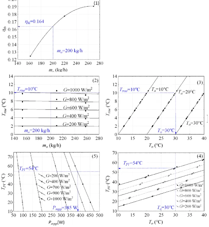
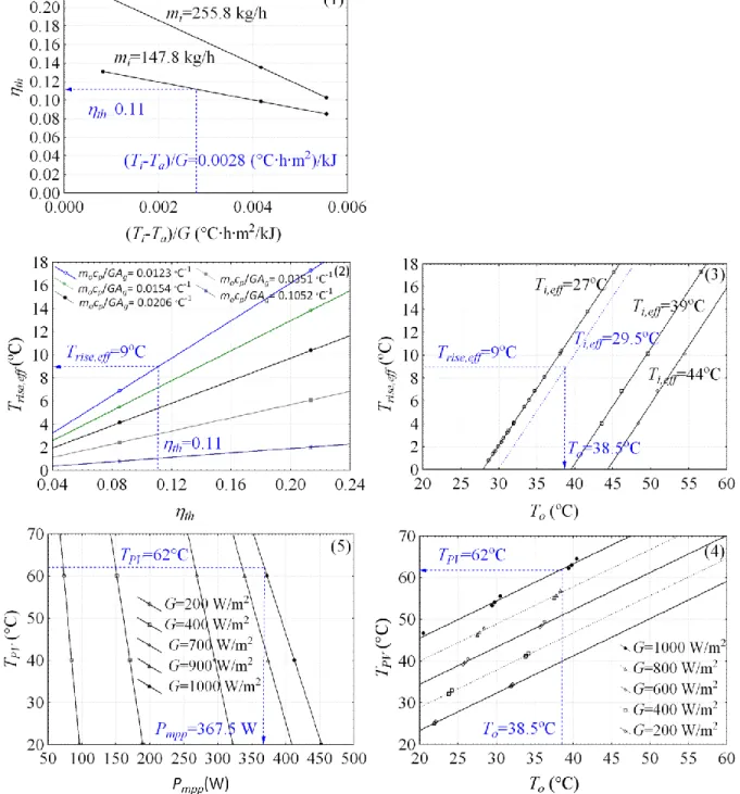
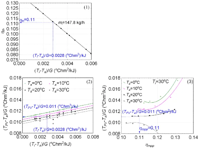
4.6.4 PV Cells Temperature Prediction Model Validation ... 51
4.6.5 PV-T Model Development for Design Purposes ... 55
4.7 Discussion ... 59 4.8 Conclusions ... 61 4.9 Acknowledgements ... 63 4.10 Nomenclature ... 63 4.11 Apendices ... 64 4.11.1 Appendix A ... 64
4.11.2 Appendix B ... 65
4.12 References ... 66
CHAPTER 5 ARTICLE 2: A NOVEL APPROACH TO COMPARE BUILDING-INTEGRATED PHOTOVOLTAICS/THERMAL AIR COLLECTORS TO SIDE-BY-SIDE PV MODULES AND SOLAR THERMAL COLLECTORS ... 69
5.1 Abstract ... 69
5.2 Keywords ... 70
5.3 Introduction ... 70
5.4 Literature Review ... 71
5.4.1 Combined Energy or Exergy Efficiency ... 71
5.4.2 Combined Primary Energy Saving Efficiency ... 73
5.4.3 Equivalent Thermal or Electrical Energy Efficiency ... 74
5.4.4 Equivalent Area ... 74
5.4.5 Combined Useful Energy ... 75
5.4.6 Economic Indicators ... 75
5.4.7 Conclusion ... 76
5.5 Methodology ... 76
5.5.1 Description of the Systems ... 78
5.5.2 BIPV-T Model and Validation ... 79
5.5.3 Other Components of the System... 91
5.5.4 System Component Costs... 91
5.5.5 Performance Indicators ... 92
5.5.6 Economic Indicators ... 95
5.6 Results and Discussion ... 95
5.6.2 Equivalent Thermal Energy Production ... 98
5.6.3 BIPV-T Break-Even Cost ... 101
5.7 Conclusions ... 108
5.8 Acknowledgements ... 109
5.9 References ... 109
CHAPTER 6 ARTICLE 3: COST-BENEFIT ANALYSIS OF INTEGRATING BIPV-T AIR SYSTEMS INTO ENERGY-EFFICIENT HOMES ... 113
6.1 Abstract ... 113
6.2 Keywords ... 114
6.3 Introduction ... 114
6.4 Literature Review ... 115
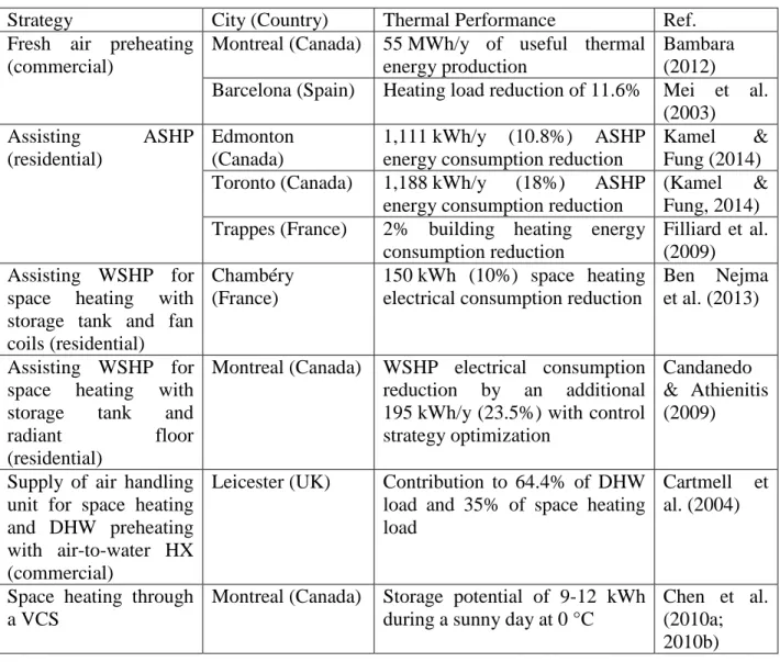
6.4.1 Fresh Air Preheating ... 116
6.4.2 Air-Source Heat Pump Coupling ... 116
6.4.3 Water-Source Heat Pump Coupling ... 117
6.4.4 Other Systems ... 117
6.4.5 Conclusion ... 118
6.5 Methodology ... 119
6.5.1 Energy-Efficient Housing Archetypes ... 120
6.5.2 Solar Energy Technology Scenarios ... 124
6.5.3 Performance Indicator ... 132
6.5.4 Economic Indicator ... 133
6.6 Results and Discussion ... 136
6.6.1 House Energy Consumption... 136
6.6.2 Useful Equivalent Energy Production ... 136
6.7 Conclusions ... 143 6.8 Acknowledgements ... 145 6.9 Nomenclature ... 145 6.10 References ... 147 6.11 Appendices ... 151 6.11.1 Appendix A ... 151 6.11.2 Appendix B ... 152 6.11.3 Appendix C ... 155
CHAPTER 7 GENERAL DISCUSSION ... 156
CHAPTER 8 CONCLUSION AND RECOMMENDATIONS ... 160
BIBLIOGRAPHY ... 163
LIST OF TABLES
Table 2-1: Steady-state thermal efficiency test required measurements ... 9
Table 2-2: Conditions for air collectors steady-state thermal efficiency measurements ... 10
Table 2-3: Values of Ross coefficient (Skoplaki et al., 2008) ... 13
Table 2-4: Values of a and b for different modules and mounting types (King et al., 2004) ... 14
Table 2-5: Indoor solar simulator minimum requirements ... 17
Table 2-6 : TRNSYS PV-T and BIPV-T models comparison ... 20
Table 2-7: Review of performance indicators used for PV-T and BIPV-T collectors and systems ... 29
Table 2-8: Review of the performance of BIPV-T and PV-T air systems ... 30
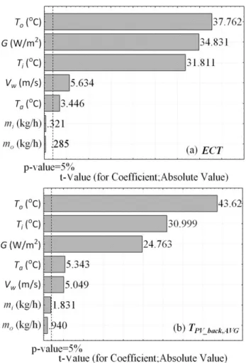
Table 4-1: Comparison of the electrical efficiency model performance using TPV=TPV_back,AVG and TPV=ECT ... 47
Table 4-2 : Thermal efficiency model coefficients ... 50
Table 4-3: Model performance comparison at predicting TPV ... 53
Table 4-4: Multiple linear regression model performance at predicting TPV ... 53
Table 4-5: Comparison of the PV electrical efficiency models performance using TPV calculated with the 3-variable multiple linear regression models of Table 4-4 ... 54
Table 5-1: Summary of models used to compute natural and forced convective heat transfer coefficients ... 85
Table 5-2: Parameters used for the model validation ... 86
Table 5-3: Matrix of the maximum power point as a function of TPV and G ... 87
Table 5-4: Scenarios for computing hnat, hw, hconv,T and hf that showed the most potential ... 87
Table 5-5: Parameters used for the solar thermal collector ... 91
Table 5-6: Criteria for determining thermal energy usefulness ... 94
Table 6-2: Main characteristics of housing archetypes ... 122
Table 6-3: Locations of housing archetypes ... 123
Table 6-4: Envelope properties for selected locations ... 123
LIST OF FIGURES
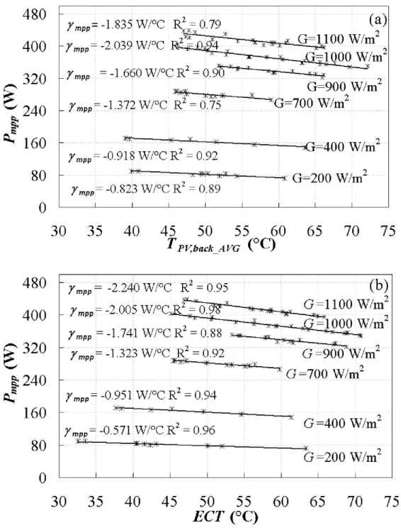
Figure 4-1: BIPV-T collector testing loop schematic ... 44 Figure 4-2: PV-T collector mounted on the outdoor combined PV and thermal testing rig ... 45 Figure 4-3: PV maximum power point for various irradiance levels as a function of (a)
TPV_back,AVG (b) ECT ... 48 Figure 4-4: Thermal efficiency in closed-loop as a function of (a) (Ti-Ta)/G (b)
(To-Ta)/G (c) (Tfm-Ta)/G ... 50 Figure 4-5: Thermal efficiency in open-loop as a function of outlet flowrate ... 51 Figure 4-6: Pareto diagrams identifying the most important variables in the prediction of (a) ECT
and (b) TPV_back,AVG ... 52 Figure 4-7: Comparison of the measured and predicted electrical efficiencies using TPV calculated
with the 3-variable multiple linear regression model ... 54 Figure 4-8: 5-plot system representing the PV-T collector performance in open-loop
configuration ... 57 Figure 4-9: 5-plot system representing the PV-T collector in closed-loop ... 59 Figure 4-10: 3-plot system adapted from the IEA to represent the PV-T collector in a closed-loop
configuration ... 60 Figure 5-1: Schematic of systems ... 78 Figure 5-2: BIPV-T system thermal resistance network ... 80 Figure 5-3: Comparison of the predicted and measured (a) thermal and (b) electrical efficiency,
ηth and ηel, using the best scenarios for computing the fluid top convective heat transfer coefficient, hconv,T and the fluid heat transfer coefficient, hf ... 89 Figure 5-4: (a) Mean bias error and (b) root mean square error in predicting the fluid outlet
temperature, To, the PV cells’ temperature, TPV, the thermal efficiency, ηth, and the electrical efficiency, ηel, for the 8 best scenarios for computing the fluid heat transfer coefficient, hf and the fluid top convective heat transfer coefficient, hconv,T ... 90
Figure 5-5: Comparison of the energy produced by the BIPV-T and the PV+T systems for a
40 m2 roof in Montreal and Tw,in=Tmains ... 96
Figure 5-6: Comparison of the energy produced by the BIPV-T and the PV+T systems for a 40 m2 roof in Montreal and Tw,in=10 °C ... 97
Figure 5-7: Comparison of the energy produced by the BIPV-T and the PV+T systems for a 40 m2 roof in Montreal and Tw,in=20 °C ... 98
Figure 5-8: Ratio of equivalent useful thermal energy between the BIPV-T and PV+T systems for a 40 m2 roof in Montreal and Tw,in=Tmains ... 99
Figure 5-9: Ratio of equivalent useful thermal energy between the BIPV-T and PV+T systems for a 40 m2 roof in Montreal and Tw,in=10 °C ... 100
Figure 5-10: Ratio of equivalent useful thermal energy between the BIPV-T and PV+T systems for a 40 m2 roof in Montreal and Tw,in=20 °C ... 101
Figure 5-11: Cost required to recover the heat from the BIPV-T system to break-even with the cost of the PV+T system for a 40 m2 roof in Montreal and Tw,in=Tmains ... 103
Figure 5-12: Cost required to recover the heat from the BIPV-T system to break-even with the cost of the PV+T system for a 40 m2 roof in Montreal and Tw,in=10 °C ... 104
Figure 5-13: Cost required to recover the heat from the BIPV-T system to break-even with the cost of the PV+T system for a 40 m2 roof in Montreal and Tw,in=20 °C ... 105
Figure 5-14: Ratio of equivalent useful thermal energy between the BIPV-T and PV+T systems as a function of the cost required to recover the heat from the BIPV-T system to break-even with the cost of the PV+T system for a 40 m2 roof in Montreal and Tw,in=Tmains ... 106
Figure 5-15: Ratio of equivalent useful thermal energy between the BIPV-T and PV+T systems as a function of the cost required to recover the heat from the BIPV-T system to break-even with the cost of the PV+T system for a 40 m2 roof in Montreal and Tw,in=10 °C ... 107
Figure 6-1: Energy-efficient housing archetypes (view of south-facing façade) ... 121
Figure 6-2: Thermal resistance network for the BIPV-T model ... 125
Figure 6-4: Schematic of roof scenario BIPV-T System 2 ... 128
Figure 6-5: Schematic of roof scenario with BIPV-T System 3 ... 128
Figure 6-6: Schematic of roof scenario with BIPV-T System 4 ... 130
Figure 6-7: Schematic of PV+T roof scenario ... 131
Figure 6-8: Energy requirements of housing archetypes by end-use ... 136
Figure 6-9: Useful equivalent electrical energy for Montreal grouped by housing archetype .... 137
Figure 6-10: Useful equivalent electrical energy for the medium 2-storey house grouped by location ... 137
Figure 6-11: Break-even and specific break-even costs compared to a BIPV system for Montreal ... 139
Figure 6-12: Break-even and specific break-even costs compared to a BIPV system for the medium 2-storey home ... 139
Figure 6-13: Break-even and specific break-even costs compared to a PV+T system for Montreal grouped by housing archetype... 140
Figure 6-14: Break-even and specific break-even costs compared to a PV+T system for the medium 2-storey home grouped by location ... 141
Figure 6-15: BIPV-T system break-even cost compared to BIPV and PV+T systems ... 143
Figure 6-16: Break-even and specific break-even costs of the BIPV-T systems compared to a BIPV system ... 152
Figure 6-17: Break-even and specific break-even costs for BIPV-T System 1 compared to a PV+T system ... 153
Figure 6-18: Break-even and specific break-even costs for BIPV-T System 2 compared to a PV+T system ... 153
Figure 6-19: Break-even and specific break-even costs for BIPV-T System 3 compared to a PV+T system ... 154
Figure 6-20: Break-even and specific break-even costs for BIPV-T System 4 compared to a PV+T system ... 154
LIST OF SYMBOLS AND ABBREVIATIONS
The list of symbols and abbreviations presented in this section is applicable to Chapters 1, 2, 3, 7 and 8. The articles presented in Chapters 4 to 6 have their own nomenclature. The symbols and abbreviations used in the articles presented in Chapters 4 to 6 are described in these specific chapters.
Abbreviation
a-Si Amorphous silicon
ANSI American National Standards Institute
ASHRAE American Society of Heating, Refrigerating and Air-Conditioning Engineers BIPV Building-integrated photovoltaics
BIPV-T Building-integrated photovoltaics with thermal energy recovery CdTE Cadmium telluride
CIGS Copper indium gallium selenide
CMHC Canada Mortgage and Housing Corporation CSA Canadian Standards Association
DHW Domestic Hot Water EN European Normalization ERS EnerGuide Rating System
HVAC Heating, Ventilation and Air-Conditioning HWB Hottel-Whillier Bliss
IEC International Electrotechnical Commission ISO International Standards Organization I-V Current-Voltage
NOCT Normal Operating Cell Temperature pc-Si Polycrystalline silicon
PV Photovoltaic
PV-T Photovoltaic with thermal energy recovery STC Standard Testing Condition
TESS Thermal Energy System Specialists TRNSYS Transient System Simulation Program Symbols
Aa Aperture area [m²]
Ag Gross area [m²]
a Empirically determined coefficient establishing the upper limit for module temperature at low wind speeds in the calculation of the cell temperature [-]
a1 Coefficient in thermal efficiency equation [W/(m²·K)]
a2 Coefficient in thermal efficiency equation [W/(m²·K²)] AMa Air mass [-]
b Empirically determined coefficient establishing the upper limit for module temperature at high irradiance in the calculation of the cell temperature [-]
bu Coefficient in thermal efficiency equation [s/m] b1 Coefficient in thermal efficiency equation [W/(m²·K)] b2 Coefficient in thermal efficiency equation [W·s/(m3·K)]
C0 Empirically-determined coefficient in the calculation of the maximum power point current [-]
C1 Empirically-determined coefficient in the calculation of the maximum power point current [-]
C2 Empirically-determined coefficient in the calculation of the maximum power point
voltage [-]
C3 Empirically-determined coefficient in the calculation of the maximum power point
voltage [-]
cp Specific heat capacity [kJ/(kg·K)]
COPHP Heat pump coefficient of performance [-] E0 Reference irradiance [W/m²]
Eb Beam component of incident solar radiation [W/m²]
Ed Diffuse component of incident solar radiation [W/m²]
Ee Effective irradiance [-]
EL Long-wave in-plane radiation [W/m²]
FR∗ Solar thermal collector heat removal factor [-]
f1(AMa) PV module spectrum dependency function [-]
f2(θ) PV module incidence angle dependency function [-]
fd Fraction of diffuse irradiance used by the module [-] G In-plane solar irradiance [W/m²]
G" Net in-plane solar irradiance [W/m²] Imp Current at maximum power point [A]
Imp0 Current at maximum power point at reference conditions[A] Isc Short-circuit current [A]
Isc0 Short-circuit current at reference conditions [A]
Iscr Reference cell short-circuit current [A]
Iscr0 Reference cell short-circuit current at reference conditions [A] k Ross coefficient [K·m²/W]
ṁ Mass flow rate [kg/h]
ṁi Air inlet mass flow rate [kg/h]
ṁo Air outlet mass flow rate [kg/h] Ns Number of cells in series [cells]
Pflow Pumping power [W]
Pmp Maximum power point [W] PPV,DC DC PV system power [W] Qel Electrical energy [kWh] Qth Thermal energy [kWh] QT,P Primary energy [kWh] SF Soiling factor [-] T∗ Characteristic temperature [°C] or [K]
T0 Reference cell temperature [°C] Ta Ambient temperature [°C] or [K] Ti Fluid inlet temperature [°C] or [K] Tm Mean fluid inlet temperature [°C] or [K]
To Fluid outlet temperature [°C] or [K]
TPV Temperature of solar cells [°C]
TPVr Temperature of the reference solar cell [°C]
UL* Solar thermal collector heat loss coefficient [W/(m²·K)]
Vf Free stream wind speed in the windward side of the PV array [m/s]
Vmp Voltage at maximum power point [V]
Vmp0 Voltage at maximum power point at reference conditions [V] Voc Open-circuit voltage [V]
Voc0 Open-circuit voltage at reference conditions [V]
Vw Wind velocity [m/s]
Greek Symbols
α Absorptance [-]
αImp Maximum power point current temperature coefficient [A/°C] αIsc Short-circuit current temperature coefficient [A/°C]
αIscr Reference cell short-circuit current temperature coefficient [A/°C]
βVmp Maximum power point voltage temperature coefficient [V/°C] βVoc Open-circuit voltage temperature coefficient [V/°C]
ε Emissivity [-]
γPmp,rel Maximum power point relative temperature coefficient [1/°C]
η0 Maximum thermal efficiency [-]
ηel Electrical efficiency [-] ηel,net Net electrical efficiency [-] ηfan Fan efficiency [-]
ηgen,grid Grid efficiency [-]
ηmotor Motor efficiency [-]
ηp→th Efficiency for converting primary energy to thermal energy [-] ηPV,system PV system efficiency [-]
ηth Thermal efficiency [-]
ηth,eq Equivalent thermal efficiency [-] ηT,net Net combined efficiency [-]
σ Stefan-Boltmann constant [W/(m²·K4)] θ Incidence angle [°]
()e Effective transmittance-absorptance product [-]
ω Ratio of Ross coefficients [-]
CHAPTER 1
INTRODUCTION
In 2014, photovoltaic (PV) technology provided 1.1% of the total electricity consumption worldwide (IEA PVPS, 2015) with an installed capacity of 177 GW. In Canada, it is 0.4% of the total electricity that was supplied by solar PV during that same year. Despite this modest penetration, the PV market is growing fast. In 2014, the total installed PV capacity in Canada was 1.84 GW (Poissant & Bateman, 2014) corresponding to 1.5 times the capacity installed in 2013 and 2.4 times that recorded in 2012. This market growth can be explained by the attractive incentives programmes that were launched in recent years (e.g., the Ontario feed-in tariff) combined with the drop in PV module prices, from 5.5 CAD/Wp in 2004 to 0.85 CAD/Wp in 2014 (Poissant & Bateman, 2014). For grid-connected distributed systems which mainly consist of PV systems mounted on the roof or façade of residential and commercial buildings, additional factors have contributed to this increased interest: the levelised cost of electricity for PV that has reached or is about to reach grid parity in some locations in Canada and the need or will of building owners to comply to specific energy consumption targets. Achieving low levels of energy consumption, especially aggressive ones such as net-zero, cannot be possible with only energy conservation and energy efficiency measures. It also requires the optimal integration of renewable energy technologies such as solar thermal and solar PV.
Standard (non-concentrated) PV modules typically convert between 7% (amorphous-silicon) to 16% (cadmium telluride) of the incident solar energy into electricity. The rest of the energy is either reflected or converted into heat if the photons have an energy level not within the band gap of the solar cells. This heat is generally lost to the surroundings and is unwanted since it contributes to increasing the temperature of the cells and reducing their efficiency. In a photovoltaic module with thermal energy recovery (PV-T), the heat generated by the solar cells is recovered either actively or passively by a heat recovery fluid that can be a liquid or air instead of being lost to the environment. Thus, compared to stand-alone PV modules, PV-T collectors produce both thermal and electrical energy simultaneously using the same surface area. Considering that buildings only have a limited amount of available façade or roof surface area with solar energy potential, PV-T is a promising technology when targeting a high energy performance building.
Similar to solar thermal collectors, PV-T collectors can use either liquid or air as the heat recovery fluid, can be glazed or unglazed and work either in a closed-loop or open-loop configuration. PV-T collectors can also be integrated to the building envelope. These are called building-integrated photovoltaics with thermal energy recovery (BIPV-T). BIPV-T collectors replace a component of the building envelope by acting as the roof, façade, window or curtainwall and thus, generally provide a greater aesthetic than PV-T collectors.
In Canada, a number of recent projects have demonstrated that BIPV-T collectors can fulfill part of the energy requirements of buildings. As part of Canada’s Mortgage and Housing Corporation (CMHC) Equilibrium competition, the EcoTerra Home (Noguchi et al., 2008) and the Alstonvale Home (Pogharian et al., 2008) have showed the potential of BIPV-T in energy-efficient single-family homes. The BIPV-T transpired collector integrated to the façade of the John Molson School of Business Building in Montreal (Athienitis et al., 2011) has proven that BIPV-T can be beneficial for preheating fresh air in commercial buildings. These projects all use air as the heat recovery fluid. Compared to liquids such as a water and glycol mixture, air has several disadvantages for use in solar thermal technologies. It has a lower thermal conductivity, which generally leads to a reduced thermal efficiency compared to liquid collectors. It also has a lower thermal capacity which makes it more difficult to store the thermal energy collected for a later use. In a BIPV-T application, however, the choice of air instead of liquid ensures greater safety and simplicity. Even though air leakage or infiltration might affect the thermal performance of a BIPV-T air collector, it will not create safety issues if the solar cells get in contact with the fluid as it would be the case in a liquid-based collector. In addition, when the fluid is air, it can be directly drawn from outdoors and work in open-loop avoiding the complexity of a closed-loop system.
Despite their great potential, PV-T and BIPV-T technologies remain niche markets. Several barriers to their market uptake have been identified in the last 10 years including the absence of performance characterization standards and product certification, the lack of information on their cost-benefit, the high cost, the absence of tools to estimate their yield and the lack of whole system solution sets (Goetzler et al., 2014; Zondag, 2008).
The work presented in this document aims at removing some of these barriers to the market uptake of BIPV-T technology by increasing the knowledge on both its performance
characterization and its true benefit. Understanding the actual value of BIPV-T compared to standard solar technologies such as PV modules or solar thermal collectors will advance the science on its current worth. In addition, it will identify future research required for its integration into efficient buildings to become common practice.
The work performed for this thesis has three main objectives. The first objective consists of developing and validating experimentally a model that can apply to BIPV-T and PV-T air collectors. The aim is to understand how its performance is affected by certain design characteristics as well as environmental and operating conditions. Ultimately, the goal is to implement it in an energy simulation tool to study the interactions with a building and its ventilation, space heating and domestic hot water heating systems. Several models of BIPV-T or PV-T air collectors have been developed and even validated experimentally, but the results obtained are difficult to compare. The main reason is that there are no standardized methods to characterize the thermal and electrical performance of PV-T collectors.
This leads to the second objective of the study which is to address some of the issues related to the thermal and electrical performance characterization of PV-T collectors. In a PV-T collector, PV cells act as the thermal absorber or as part of the thermal absorber and as a result, the thermal performance is affected by the electrical performance and vice-versa. Therefore, the application of separate PV and solar thermal collector standard performance test procedures are not sufficient to characterize the performance of PV-T collectors.
The validated model is used to fulfill the third objective of this study, which is to develop a methodology to identify the true benefit of integrating BIPV-T air collectors in high performance residential buildings compared to standard solar technologies such as PV modules and solar thermal collectors. Performing such comparison is not straightforward for BIPV-T air collectors because two types of energy having different values are generated and several performance indicators can be used. In fact, studies that have looked at quantifying the benefits of PV-T or BIPV-T air collectors show a very large spectrum of results.
CHAPTER 2
LITERATURE REVIEW
This literature review presents an overview of the research conducted on different topics related to PV-T or BIPV-T technology. More specifically, it addresses the three objectives described in Chapter 1. It is divided in two main sections. Section 2.1 discusses the different methods to characterize the performance of solar technologies and the models currently available in simulation tools. Section 2.2 focuses on a review of the approaches taken to quantify the benefit of photovoltaics with heat recovery and how it compares with more common solar energy technologies.
2.1 Performance Characterization of Solar Technologies
Standardized methods to measure and present the performance of a product are of great importance for any technology. Universal performance testing methods ensure that two products can be directly compared because both the metrics employed and the experimental procedures followed to obtain these metrics are the same. The added benefit is that the parameters and performance indicators measured during performance characterization can often be used in simplified models to predict the technology yield under specific conditions. This section presents an overview of the methods typically used to characterize the performance of solar thermal and PV technologies and discusses the additional challenges with combined photovoltaic and thermal technologies. It also includes a review of PV-T and BIPV-T models available in common whole-building simulation tools.
2.1.1 Solar Thermal Collectors
There are many different types of solar thermal collectors: liquid-based, air-based, glazed, unglazed, concentrators, open-loop and closed-loop. The variables influencing the performance of a solar thermal collector will depend on the heat transfer fluid, the presence of glazing, the design (e.g., concentrator, flat-plate, sheet-and-tube, etc.), the type of inlet (multiple entries or one single entry) and the collector operating mode (open-loop vs closed-loop).
The simplest representation of the thermal efficiency, 𝜂𝑡ℎ, of a non-concentrating solar thermal collector operated under steady-state conditions is given by the Hottel-Whillier Bliss (HWB) equation (Hottel & Whillier, 1958):
𝜂𝑡ℎ = 𝐹𝑅∗(𝜏𝛼)𝑒− 𝐹𝑅∗𝑈𝐿∗(
𝑇∗− 𝑇 𝑎
𝐺 ) (2-1)
In Equation (2-1), 𝑈𝐿∗ is the collector heat loss coefficient, 𝐹𝑅∗ is the heat removal factor and (𝜏𝛼)𝑒 is the collector effective transmittance-absorptance product. The term (𝑇∗− 𝑇𝑎) 𝐺⁄ is
known as the reduced temperature where 𝑇𝑎 is the ambient temperature, 𝐺 is in the in-plane solar irradiance and 𝑇∗ is a characteristic temperature. In North America, this characteristic temperature is generally the fluid inlet temperature, 𝑇𝑖. In European and international standards, however, it is more common to use the fluid mean temperature, 𝑇𝑚. This mean fluid temperature is calculated as the arithmetic average of the fluid inlet (𝑇𝑖) and outlet (𝑇𝑜) temperatures. The heat
loss coefficient, 𝑈𝐿∗, is not always constant and for some flat-plate collectors, can be a function of
𝑇∗− 𝑇
𝑎 as shown by Gordon (1981). In that case, the term 𝐹𝑅∗𝑈𝐿∗ in Equation (2-1) becomes
𝐹𝑅∗𝑈
𝐿∗ = 𝑎1+ 𝑎2(𝑇∗− 𝑇𝑎) (2-2)
where 𝑎1 and 𝑎2 are constants. By substituting Equation (2-2) in the thermal efficiency relation shown in Equation (2-1), 𝜂𝑡ℎ can be expressed as
𝜂𝑡ℎ = 𝐹𝑅∗(𝜏𝛼)𝑒− 𝑎1( 𝑇∗− 𝑇 𝑎 𝐺 ) − 𝑎2 (𝑇∗− 𝑇 𝑎)2 𝐺 (2-3) or 𝜂𝑡ℎ = 𝜂0− 𝑎1(𝑇∗− 𝑇𝑎 𝐺 ) − 𝑎2 (𝑇∗− 𝑇 𝑎)2 𝐺 (2-4)
In Equation (2-4), 𝜂0 is the collector maximum efficiency obtained when 𝑇∗= 𝑇𝑎. Equations (2-1) and (2-4) are generally only valid for glazed collectors. The steady-state efficiency for unglazed collectors or for collectors with the heat recovery fluid in direct contact with the cover is slightly different. In these particular products, the heat recovery fluid temperature is much more influenced by the collector convective and radiative heat losses to the surroundings. As a result, the wind speed and long-wave radiation have a greater effect on the performance and they need to be taken into account in the efficiency equation. The long-wave radiation, 𝐸𝐿, is
accounted for by using the net incident solar radiation, 𝐺", as opposed to the in-plane solar irradiance in the calculation of the thermal efficiency. 𝐺" is defined as:
𝐺" = 𝐺 +𝜀
𝛼(𝐸𝐿− 𝜎𝑇𝑎4) (2-5)
In Equation (2-5), 𝜀 𝛼⁄ is the collector emissivity over absorptance ratio, 𝜎 is the Stefan-Boltzmann constant and 𝑇𝑎 is the ambient temperature in Kelvins. As for the wind effect, it is accounted for by expressing 𝐹𝑅∗(𝜏𝛼)𝑒 and 𝐹𝑅∗𝑈𝐿∗ as linear functions of wind velocity, 𝑉𝑤, as
shown in Harrison et al. (1989): 𝐹𝑅∗(𝜏𝛼)
𝑒 = 𝜂0(1 − 𝑏𝑢𝑉𝑤) (2-6)
𝐹𝑅∗𝑈
𝐿∗= (𝑏1+ 𝑏2𝑉𝑤) (2-7)
In Equations (2-6) and (2-7), 𝑏𝑢, 𝑏1 and 𝑏2 are constants. Hence, the thermal efficiency of unglazed collectors (or collectors where the fluid is in direct contact with the glazing) is given by:
𝜂𝑡ℎ = 𝜂0(1 − 𝑏𝑢𝑉𝑤) − (𝑏1+ 𝑏2𝑉𝑤) (
𝑇∗− 𝑇 𝑎
𝐺" ) (2-8)
The efficiency relations given in Equations (2-1), (2-4) and (2-8) are applicable to both liquid or air collectors, but are only valid for a specific flowrate in the case of air collectors. As explained by Kramer (2013), the main difference between air and liquid collectors is that the heat transfer coefficient between the absorber and the fluid is much lower in an air collector and much more dependent on flowrate. In an air collector, the lower the flowrate, the higher is the temperature of the absorber and the higher are the collector convective and radiative losses to the surroundings. Another difference between liquid and air collectors is that air collectors are never perfectly sealed and the amount of air leaking from or infiltrating the collector affects its performance (Bernier & Plett, 1988). In a liquid-based collector, the thermal efficiency is given by
𝜂𝑡ℎ =
𝑚̇𝑐𝑝(𝑇𝑜− 𝑇𝑖)
where 𝐴𝑎 is the collector aperture area and 𝑐𝑝and 𝑚̇ represent the fluid heat specific heat and flowrate, respectively. In an air collector, however, air leakage is related to its operating gauge pressure. If the collector operates under negative pressure relative to the ambient, ambient air will be infiltrating the collector. On the opposite, if the collector operates under positive pressure, air will be leaking from the collector. As a result, the thermal efficiency of an air-based solar thermal collector is calculated using:
𝜂𝑡ℎ = 𝑚̇𝑜𝑐𝑝(𝑇𝑜− 𝑇𝑖) + (𝑚̇𝑜− 𝑚̇𝑖)𝑐𝑝(𝑇𝑖 − 𝑇𝑎)
𝐺𝐴𝑎 (2-10)
In Equation (2-10), the subscripts 𝑖 and 𝑜 refer to the collector inlet and outlet, respectively. For unglazed solar thermal collectors, Equations (2-9) and (2-10) can still be used, but 𝐺 is replaced by 𝐺". Note that 𝐺 (or 𝐺") must be multiplied by a conversion factor corresponding to 3.6 kJ/(h·W) if the units in the nomenclature are used.
Several standards provide performance and reliability test methods for solar thermal collectors. The most common ones applicable to air collectors are:
ANSI/ASHRAE 93-2010 “Methods of Testing to Determine the Thermal Performance of Solar Collectors” (ASHRAE, 2010)
CAN/CSA-F378 Series-11 “Solar Collectors” (CSA, 2012)
ISO 9806 “Solar thermal collectors – Test methods” (ISO, 2013)
The standard ANSI/ASHRAE 93-2010 mostly focuses on performance testing with test procedures to obtain air leakage rate, steady-state thermal efficiency, time constants and incidence angle dependence. In addition to performance tests, CAN/CSA-F378 Series-11 and ISO 9806 also contain reliability tests including, but not limited to, external thermal shock, exposure, high-temperature resistance and mechanical load. All three standards contain indoor and outdoor testing procedures. The standard ANSI/ASHRAE 93-2010 applies only to glazed collectors, but CAN/CSA-F378 Series-11 and ISO 9806 are applicable to both glazed and unglazed products. In the case of ISO 9806, it can even be used for glazed and unglazed PV-T collectors, referred to as hybrid collectors. In this standard, a PV-T collector is considered unglazed when the absorber “is close connected to the electricity generation and if there is no extra glazing in front” (ISO, 2013). For PV-T collectors, it is specified that testing can be done
with the PV operating at maximum power point, in open-circuit or even in short-circuit conditions as long as the PV operating mode is mentioned in the test report.
The test loops, instruments and measurements recommended in the different standards are similar. In ANSI/ASHRAE 93-2010, a test loop having both upstream and downstream sections is required. Each section has airflow, temperature and pressure measuring stations to account for air leakage or infiltration. A pre-conditioning apparatus is located at the collector inlet to allow regulating the fluid inlet temperature. A similar testing loop is recommended in CAN/CSA-F378 Series-11, but only one flowrate measurement is mandatory. In ISO 9806, distinct testing loops are required depending on whether the collector is typically used in a closed-loop or open-loop configuration. The closed-loop is similar to that proposed in ANSI/ASHRAE 93-2010.
A comparison of the measurements required by the three standards during the steady-state thermal efficiency test is shown in Table 2-1. The main differences are that the CAN/CSA F378 Series-11 standard requires only one flowrate measurement and ISO 9806 for open-loop collectors requires fewer measurements since the test loop only has a downstream section. In addition, ISO 9806 does not require that the wind direction be measured. In all standards, it is recommended to use a pyranometer for short-wave irradiance measurement and a pyrheliometer for direct normal irradiance.
Table 2-1: Steady-state thermal efficiency test required measurements ANSI/ASHRAE 93-2010 CAN/CSA F378 Series-11 ISO 9806 Closed-loop Open-loop Ambient pressure X X X
Ambient air temperature X X X X
Humidity ratio X X X X
Inlet gauge pressure X X X
Outlet gauge pressure X X X X
Differential pressure X X X
Inlet fluid temperature X X X
Outlet fluid temperature X X X X
Fluid temperature rise X X X X
Inlet flowrate X X
Outlet flowrate X X1 X X
In-plane short-wave irradiance
X X X X
Direct normal irradiance (outdoor testing)
X X X X
In-plane long-wave irradiance
X2 X2 X3 X3
Surrounding air speed X X X X
Surrounding air direction X X
The inlet temperature, flowrate and wind speed conditions under which the steady-state thermal efficiency of air collectors should be measured vary between standards. These are summarized in Table 2-2.
1
Only one air flowrate is required, either at the inlet or outlet
2 Only necessary for indoor testing
3 The in-plane long-wave irradiance can also be calculated if it cannot be measured. Procedures are given in the
Table 2-2: Conditions for air collectors steady-state thermal efficiency measurements ANSI/ASHRAE 93-2010 CAN/CSA F378 Series-11 ISO 9806 Inlet temperature 4 values of (𝑇𝑖 − 𝑇𝑎): 0%, 30%, 60% and 90% of the value of (𝑇𝑖 − 𝑇𝑎) at a given
temperature
Open-loop: 𝑇𝑖 = 𝑇𝑎 Closed-loop:
4 values of 𝑇𝑚 with one value such that
𝑇𝑚= 𝑇𝑎+ 3 K
Flowrate 0.01 m3/(s·m2)4 0.03 m3/(s·m2)
2 values: min and max values recommended by the manufacturer 3 values: between 30 to 300 kg/(h·m2)4 or as recommended by the manufacturer Wind speed Glazed – indoor:
3 to 4 m/s Glazed – outdoor: 2 to 4 m/s Glazed – indoor: 3 to 4 m/s Glazed – outdoor: 2 to 4 m/s Unglazed – indoor: 0.75 to 1 m/s, 1.5 to 2 m/s and >2.5 m/s Unglazed – outdoor: 2 to 4.5 m/s Glazed: 2 to 4 m/s Unglazed: <1 m/s, 1 to 2 m/s and 2.5 to 3.5 m/s
2.1.2 PV Modules
The performance of a PV Module can be characterized by its current-voltage (I-V) curve. On this curve, three points can be identified: the short-circuit current (𝐼𝑠𝑐), the open-circuit voltage (𝑉𝑜𝑐) and the maximum power point (𝑃𝑚𝑝). This maximum power point is the point at which the
current and voltage are such that the power produced by the PV module is maximized. The current and voltage at maximum power point are known as 𝐼𝑚𝑝 and 𝑉𝑚𝑝. These five key parameters of an I-V curve depend mainly on the incident solar radiation and cell temperature and to a secondary order, on the air mass and incidence angle as demonstrated in the model of King et al. (2004):
𝐼𝑠𝑐= 𝐼𝑠𝑐0𝐸𝑒[1 + 𝛼𝐼𝑠𝑐(𝑇𝑃𝑉− 𝑇0)] (2-11)
𝐼𝑚𝑝 = 𝐼𝑚𝑝0[𝐶0𝐸𝑒 + 𝐶1𝐸𝑒2][1 + 𝛼𝐼𝑚𝑝(𝑇𝑃𝑉− 𝑇0)] (2-12)
𝑉𝑜𝑐 = 𝑉𝑜𝑐0+ 𝑁𝑠𝛿(𝑇𝑃𝑉)ln(𝐸𝑒) + 𝛽𝑉𝑜𝑐(𝐸𝑒)(𝑇𝑃𝑉− 𝑇0) (2-13)
𝑉𝑚𝑝 = 𝑉𝑚𝑝0+ 𝐶2𝑁𝑠𝛿(𝑇𝑃𝑉)ln(𝐸𝑒) + 𝐶3𝑁𝑠[𝛿(𝑇𝑃𝑉)ln(𝐸𝑒)]2+ 𝛽𝑉𝑚𝑝(𝐸𝑒)(𝑇𝑃𝑉− 𝑇0) (2-14)
𝑃𝑚𝑝 = 𝐼𝑚𝑝𝑉𝑚𝑝 (2-15)
In Equations (2-11) to (2-15), 𝐼𝑠𝑐0, 𝐼𝑚𝑝0, 𝑉𝑜𝑐0and 𝑉𝑚𝑝0 are the short-circuit current, current at
maximum power point, open-circuit voltage and voltage at maximum power point at a reference irradiance level 𝐸0 (typically 1000 W/m2) and cell temperature 𝑇0 (typically 25 °C) for an air mass, 𝐴𝑀𝑎, of 1.5 and an incidence angle, θ, of 0°. 𝛼𝐼𝑠𝑐, 𝛼𝐼𝑚𝑝, 𝛽𝑉𝑜𝑐 and 𝛽𝑉𝑚𝑝 are the temperature coefficients for short-circuit current, current at maximum power point, open-circuit voltage and voltage at maximum power point. 𝐶0, 𝐶1, 𝐶2 and 𝐶3 are empirically-determined coefficients. 𝑇𝑃𝑉 is the solar cells temperature. Ns is the number of cells in series. 𝐸𝑒 is the effective irradiance defined as the PV module in-plane solar irradiance taking into account the solar spectral variation, the optical losses due to solar angle-of-incidence and module soiling. The most common method to obtain the effective irradiance is by measuring the short-circuit current of a calibrated reference cell (𝐼𝑠𝑐𝑟) that uses the same solar cell technology than the module under test and that is positioned at the same slope and orientation. The reference cell has identical solar spectral and incidence angle dependence as the module and the level of irradiance as seen by the PV module is calculated with:
𝐸𝑒 = 𝐼𝑠𝑐𝑟
𝐼𝑠𝑐0𝑟(1 + 𝛼𝐼𝑠𝑐𝑟(𝑇𝑃𝑉𝑟− 𝑇0))
𝑆𝐹 (2-16)
In Equation (2-16), 𝑆𝐹 is the module soiling factor and the subscript r refers to the reference cell. If instead of a reference cell, thermopile-based instruments (e.g., pyranometers or pyheliometers) are used to measure the irradiance level, the effective irradiance can still be calculated, but corrections are required to take into account the fact that the irradiance sensor(s) and module spectrum and incidence angle effect differ. In this case, 𝐸𝑒 is calculated with the following relation:
𝐸𝑒 = 𝑓1(𝐴𝑀𝑎) (
𝐸𝑏𝑓2(𝜃) + 𝑓𝑑𝐸𝑑
𝐸0 ) 𝑆𝐹 (2-17)
In Equation (2-17), 𝐸𝑏 and 𝐸𝑑 are the beam and diffuse components of incident solar radiation
and 𝑓1(𝐴𝑀𝑎) and 𝑓2(𝜃) are the module spectrum and incidence angle dependency functions. 𝑓𝑑 is
the fraction of diffuse irradiance used by the module. In the worst case scenario, these effects can be neglected and 𝐸𝑒 can simply be calculated with
𝐸𝑒 = (𝐸
𝐸0) 𝑆𝐹 (2-18)
where 𝐸 is the in-plane solar irradiance measured by a pyranometer. In Marion (2012), the effect of correcting for temperature, incidence angle and spectrum for estimating daily efficiencies of four PV modules of different technologies is studied. Two different spectrum correction methods are tested: a complex model that accounts for the spectral irradiance and spectral response of both the modules and irradiance sensor for each wavelength and a simpler model that uses the air mass correction factor developed by Sandia National Laboratory (King et al., 2004) corresponding to 𝑓1(𝐴𝑀𝑎) in Equation (2-17). It was found that the daily efficiency standard deviation was the
lowest when correcting for temperature, incidence angle and spectrum with the complex method. Using the air mass correction factor, however, the results were improved only for the mono-crystalline module and only slightly for the CIGS module. They were worst for the CdTe and a-Si/a-Si/a-Si:Ge PV modules. This was explained by the fact that these two modules are much more sensitive to water vapor that is not taken into account in the simple air mass correction 𝑓1(𝐴𝑀𝑎).
Simpler models than that developed by King et al. can be used to predict the maximum power point of PV modules. One of the simplest models is that used in the software PVFORM (Menicucci & Fernandez, 1988) and is given as:
For 𝐸𝑒>125 W/m2:
𝑃𝑚𝑝= 𝐸𝑒𝑃𝑚𝑝0[1 + 𝛾𝑃𝑚𝑝,𝑟𝑒𝑙(𝑇𝑃𝑉− 𝑇0)] (2-19)
For 𝐸𝑒≤125 W/m2
𝑃𝑚𝑝 =
0.008(𝐸𝑒𝐸0)2
𝐸0 [1 + 𝛾𝑃𝑚𝑝,𝑟𝑒𝑙(𝑇𝑃𝑉− 𝑇0)] (2-20)
In Equations (2-19) and (2-20), 𝛾𝑃𝑚𝑝,𝑟𝑒𝑙 is the relative maximum power point temperature coefficient. As it can be observed in the models presented, the cell temperature is a key input to the prediction of the performance of PV modules. This temperature is generally determined from the ambient temperature, irradiance level, wind speed, solar cell technology and mounting configuration. Several models have been developed for predicting the temperature of PV cells. The simplest equation for steady-state operating temperature of a PV module under no wind conditions is
𝑇𝑃𝑉 = 𝑇𝑎+ 𝑘𝐺 (2-21)
where 𝑘 is the Ross coefficient (Ross, 1976). This coefficient expresses the temperature rise above ambient with increasing solar flux:
𝑘 =∆(𝑇𝑃𝑉− 𝑇𝑎)
∆𝐺 (2-22)
A summary of typical Ross coefficients for different mounting configurations is given in Table 2-3.
Table 2-3: Values of Ross coefficient (Skoplaki et al., 2008)
Mounting type 𝑘
(K·m2/W)
Free standing 0.021
Flat roof 0.026
Sloped roof: well cooled 0.020
Sloped roof: not so well cooled 0.034
Sloped roof: highly integrated, poorly ventilated 0.056
Façade integrated: transparent PV 0.046
Façade integrated: opaque PV, narrow gap 0.054
In Skoplaki et al. (2008), the effect of wind on the cell temperature is introduced with a modified version of Equation (2-21) that takes into account the free stream wind speed in the windward side of the PV array, 𝑉𝑓:
𝑇𝑃𝑉 = 𝑇𝑎+ 𝜔 (
0.32
8.91 + 2𝑉𝑓) 𝐺 (2-23)
In Equation (2-23), 𝜔 is the ratio of the Ross coefficient for the specific mounting configuration to the Ross coefficient on the free-standing case:
𝜔 = 𝑘𝑓𝑟𝑒𝑒 𝑠𝑡𝑎𝑛𝑑𝑖𝑛𝑔
𝑘𝑚𝑜𝑢𝑛𝑡𝑖𝑛𝑔 𝑡𝑦𝑝𝑒 (2-24)
In King et al. (2004), the back surface module temperature is estimated with the following relation
𝑇𝑃𝑉 = 𝑇𝑎+ 𝐺(𝑒𝑎+𝑏𝑉𝑓) (2-25)
In Equation (2-25), 𝑎 and 𝑏 are empirically determined coefficients establishing the upper limit for module temperature at low wind speeds and high irradiance and the rate at which the module temperature drops as wind speed increases, respectively. Table 2-4 provides examples of values for these coefficients obtained for different modules and mounting types.
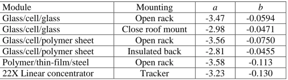
Table 2-4: Values of a and b for different modules and mounting types (King et al., 2004)
Module Mounting a b
Glass/cell/glass Open rack -3.47 -0.0594
Glass/cell/glass Close roof mount -2.98 -0.0471 Glass/cell/polymer sheet Open rack -3.56 -0.0750 Glass/cell/polymer sheet Insulated back -2.81 -0.0455 Polymer/thin-film/steel Open rack -3.58 -0.113
22X Linear concentrator Tracker -3.23 -0.130
The methodology required to obtain the different electrical parameters characterizing a PV module is described in the two international standards IEC 61215 (IEC, 2005) and IEC 61646 (IEC, 1998) focusing on the design qualification and type approval of crystalline silicon and thin-film terrestrial PV modules, respectively. In these standards, indoor and outdoor procedures are given to obtain the PV module power, efficiency, current and voltage at maximum power point along with the short-circuit current and open-circuit voltage at Standard Testing Condition
(STC), Normal Operating Cell Temperature (NOCT) and Low Irradiance Condition (LIC). These conditions are as follows:
STC: Irradiance level of 1000 W/m2, module temperature of 25 °C and a solar spectrum of air mass 1.5
NOCT: Irradiance level of 800 W/m2, ambient temperature of 20 °C, wind speed of 1 m/s, module tilted at 45° and a solar spectrum of air mass 1.5
LIC: Irradiance level of 200 W/m2, module temperature of 25 °C and a solar spectrum of air mass 1.5
Procedures are also given to obtain the temperature coefficients for current, voltage and peak power. In order to perform these different tests, the following measurements must be made:
Irradiance with a calibrated reference cell
Current and voltage of the PV reference device and PV module under test
Temperature of the module cells and PV reference device
Wind speed and direction
Ambient temperature
2.1.3 PV-T Technology
Sections 2.1.1 and 2.1.2 showed that the electrical yield of PV modules and the thermal yield of solar thermal collectors are influenced by different variables. The thermal efficiency of air solar thermal collectors is mainly influenced by the reduced temperature, the flowrate, the incidence angle and for unglazed collectors, by the wind speed. As for the amount of electricity produced by PV modules, it essentially depends on the irradiance level and cell temperature and to a second degree order, on the solar spectrum and incidence angle.
The thermal yield of PV-T collectors is influenced by the same variables than solar thermal collectors, but it is also affected by the amount of electricity produced by the PV cells. As for the electrical yield, it depends on the irradiance level, cell temperature, solar spectrum and incidence angle as in a PV module, but in PV-T collectors, the temperature of the cells does not depend only on ambient conditions and mounting configuration. It is also affected by the heat recovery
fluid temperature. The relation between the cell and the heat recovery fluid temperatures cannot be encapsulated solely with the reduced temperature. As shown in Tripanagnostopoulos et al. (2002), the electrical efficiency of a PV-T collector would depend only on the reduced temperature if the ambient temperature and incident solar radiation were kept constant during the experiment.
This interaction between the thermal and electrical yield of a PV-T collector is one of the issues with their performance characterization. Additional challenges were identified by the European initiative PV Catapult (2005) which produced a guide to highlight the main issues with PV-T collector performance testing and suggest elements to incorporate into the standards IEC 61215 (IEC, 2005) and EN 12975-2 (ECS, 2005) (the European standard for solar thermal collector testing) to address these issues. The guideline focused on non-concentrating liquid PV-T collectors using c-Si PV cells. One of the main issues discussed in this document is whether or not thermal and electrical measurements should be done separately or simultaneously in a PV-T collector since the thermal performance influences the electrical performance and vice-versa. Taking thermal measurements with the PV short-circuited or in open-circuit would later require the introduction of a thermal performance correction factor to account for the fact that in reality, the collector also produces electricity. PV Catapult concluded that since this factor was probably not straightforward to obtain, the collector should be producing electricity when taking thermal measurements and that it should be operating at its maximum power point. I-V curves should still be taken at regular time intervals, however, to simultaneously collect data for the electrical performance characterization. This is in contradiction with the standard ISO 9806 (ISO, 2013) that leaves it up to the manufacturer or testing facility to decide if the PV module during PV-T collector thermal testing should operate at maximum power point, in open-circuit or in short-circuit conditions.